The dynamics of convective orographic precipitation : the transition to convection

(1)

Universidade de Lisboa

Faculdade de Ciências

Departamento de Engenharia Geográfica, Geofísica e Energia

The dynamics of convective orographic precipitation: the transition to

convection

Miguel Nogueira

Doutoramento em Ciências Geofísicas e da Geoinformação

(Meteorologia)

(2)

Universidade de Lisboa

Faculdade de Ciências

Departamento de Engenharia Geográfica, Geofísica e Energia

The dynamics of convective orographic precipitation: the transition to

convection

Miguel Nogueira

Tese orientada por:

Professor Doutor Pedro M. A. Miranda

Professora Doutora Ana P. Barros

Tese especialmente elaborada para a obtenção do grau de Doutor em Ciências

Geofísicas e da Geoinformação (Meteorologia)

(3)

(4)

Acknowledgements

I would like to thank both my advisors, Professor Pedro Miranda and Professor Ana Barros for their scientific guidance, support and for providing me with the opportunity to work in two fantastic research teams, both at Instituto Dom Luiz at the University of Lisbon and also at Duke University. I want to acknowledge all my colleagues in both groups with whom I had the pleasure of spending these past years. In particular I am grateful to Jing Tao for her tireless help with the hydrological modeling experiments and to Xiaoming Sun for sharing his remarkable WRF simulation efforts over the Andes.

I acknowledge the funding I received from the Fundação para a Ciência e Tecnologia (F.C.T.) under doctoral grant SFRH/BD/61148/2009. I also acknowledge the funding I received from project SMOG (Structure of MOist convection in high-resolution GNSS observations and models) funded by the Portuguese Science Foundation (PTDC/CTE-ATM/119922/2010) and project IPHEx (Integrated Precipitation and Hydrology Experiment) at Professor Barros research group at Duke University during this final year of my PhD, supported by NASA grant NNX13AH39G.

Agradeço todo o apoio que recebi da minha mãe, pai, avó e irmão, à família Albergaria e aos meus amigos. Finalmente agradeço à Raquel pelo apoio incondicional sem o qual não teria possível chegar aqui e ao Francisco pela enorme alegria que nos trouxe ao longo destes últimos meses.

(8)

Abstract

Multifractal behavior holds to a remarkable approximation over wide ranges of spatial scales in orographic rainfall and cloud fields. The scaling exponents characterizing this behavior are shown to be fundamentally transient with nonlinear dependencies on the particular atmospheric state and terrain forcing. In particular, a robust transition is found in the scaling parameters between non-convective (stable) and convective (unstable) regimes, with clear physical correspondence to the transition from stratiform to organized convective orographic precipitation. These results can explain two often reported scaling regimes for atmospheric wind, temperature and water observations. On the one hand, spectral slopes around 2-2.3 arise under non-convective or very weak convective conditions when the spatial patterns are dominated by large-scale gradients and landform. On the other hand, under convective conditions the scaling exponents generally fluctuate around 5/3, in agreement with the Kolmogorov turbulent regime accounting for the intermittency correction.

High-resolution numerical weather prediction (NWP) models are able to reproduce the ubiquitous scaling behavior of observed atmospheric fields down to their effective resolution length-scale, below which the variability is misrepresented by the model. The effective resolution is shown to be a transient property dependent on the particular simulated conditions and NWP formulation, implying that a blunt decrease in grid spacing without adjusting numerical techniques may not lead to the improvements desired.

Finally, the application of transient spatial scaling behavior for stochastic downscaling and sub-grid scale parameterization of cloud and rainfall fields is investigated. The proposed fractal methods are able to rapidly generate large ensembles of high-resolution statistically robust fields from the coarse resolution information alone, which can provide significant improvements for stochastic hydrological prediction and associated extreme event forecasting and risk management, and also for stochastic sub-grid parameterization of clouds with large potential to improve the current state-of-the-art cloud parameterization schemes.

KEYWORDS: orographic precipitation; convection; multifractals; stochastic parameterization; downscaling.

(9)

Resumo

A presente tese focou-se na dinâmica da precipitação orográfica, com particular interesse na transição para o regime convectivo que pode ser responsável por eventos de precipitação extrema, com riscos naturais importantes associados como inundações rápidas, deslizamentos de terras e avalanches de sedimentos. Os eventos de precipitação convectiva representam um enorme desafio do ponto de vista da previsão operacional devido ao seu carácter turbulento, com estrutura localizada e altamente transiente. Os modelos lineares conseguem explicar algumas propriedades importantes da iniciação de convecção e estrutura espacial dos campos resultantes de precipitação e nuvens orográficas, no entanto não conseguem fazer qualquer previsão quantitativa e só conseguem prever qualitativamente a estrutura (aproximadamente) correta em casos muito particulares. Isto deve-se essencialmente ao facto da importância de inúmeras interações não lineares na dinâmica destes eventos não poder ser ignorada. No presente estudo, investigou-se a estrutura multifractal dos campos de nuvens e precipitação orográfica, representando uma aproximação notável para as observações consideradas numa vasta gama de escalas espaciais desde comprimentos da ordem de 1 km até valores superiores a 500 km, capaz de representar a estrutura complexa destes campos com variabilidade numa vasta gama de escalas, resultante da interação de diversos processos não lineares com forte influência orográfica. Mostrou-se que o comportamento multifractal é deformando pela presença de numerosos zeros, característicos em campos de nuvens e precipitação devido à presença de limiares associados às transições de fase e outros efeitos não lineares. Utilizou-se análise de clusters para isolar as regiões chuvosas (i.e. regiões conexas sem zeros) realizando a análise multifractal apenas nestas regiões, recuperando a sua estrutura multifractal não deformada.

A análise multifractal de campos atmosféricos observados e simulados numericamente mostraram que os expoentes fractais que caracterizam o comportamento estocástico de invariância de escala são intrinsecamente transientes, com dependências não lineares nas condições particulares do estado da atmosfera e de forçamento topográfico. Em particular, encontraram-se ligações entre estes parâmetros e a velocidade média do vento, a forma do terreno e a estabilidade estática da atmosfera. Um resultado particularmente robusto foi a transição nos parâmetros fractais entre os regimes não-convectivo (estável) e convectivo (instável), com clara correspondência física com a transição entre precipitação orográfica

(10)

estratiforme e convectiva. Estes resultados mantêm-se válidos para análise espectral de Fourier, escalamento dos momentos estatísticos e funções estruturais, mesmo quando a deformação do comportamento multifractal devido à presença de zeros é explicitamente tomada em consideração. Estes resultados explicam dois regimes de invariância de escala amplamente encontrados em campos atmosféricos de vento, temperatura e água suas diversas fases. Por um lado, exponentes espectrais com valores de 2-2.3 surgem em situações não-convectivas ou com estruturas convectivas fracas, quando as distribuições espaciais são dominadas por gradientes de larga escala ou pela topografia. De facto, as propriedades de invariância de escala nestas situações são semelhantes ao comportamento fractal observado nos respetivos campos de elevação topográfica. Por outro lado, em condições convectivas os expoentes espectrais flutuam em torno do valor 5/3, de acordo com as previsões de Kolmogorov para o regime turbulento tomando em consideração as correções associadas à intermitência. O parâmetro de intermitência multifractal mostrou um comportamento semelhante, dando mais robustez aos resultados obtidos. Adicionalmente a simetria horizontal pode ser quebrada em certas ocasiões, gerando anisotropia horizontal no comportamento multifractal com importantes impactos nos campos atmosféricos.

Os modelos numéricos de previsão meteorológica são capazes de reproduzir o comportamento multifractal observado em campos atmosféricos até à escala correspondente à sua resolução efetiva. Abaixo desta escala a variabilidade é representada de forma errónea pelos modelos. Mostrou-se que a resolução efetiva é uma propriedade transiente que depende das condições particulares do sistema simulado e da própria formulação do modelo numérico, com particular sensibilidade a parametrização dos efeitos turbulentos de sub-escala e à difusão numérica, geralmente introduzida para manter a estabilidade das soluções numéricas. Estes efeitos tendem a causar uma remoção excessiva de variabilidade nas pequenas escalas, onde os expoentes espectrais apresentam valores não físicos superiores a 3. Nas escalas superiores à resolução efetiva o modelo representa de forma adequada a estrutura da atmosfera, mostrando que o aumento de resolução dinâmico realizado pelos modelos numéricos a partir do forçamento de resolução grosseira é capaz de conservar e representar as propriedades multifractais da atmosfera. Em particular, os resultados mostraram que nos casos convectivos o aumento de resolução de 6 km, onde um esquema de parametrização para a convecção tem que ser introduzido, para uma resolução de 1.2 km, onde as estruturas convectivas são parcialmente

(11)

resolvidas, resultou num aumento de resolução efetiva consideravelmente inferior à diminuição do espaçamento da grelha. Este resultado implica que a diminuição do espaçamento da grelha (i.e. aumento da resolução) por si só, sem um ajustar das técnicas de modelação numérica, poderá não levar à melhoria dos resultados da simulação desejados.

Investigou-se o potencial do comportamento multifractal transiente para aplicações estocásticas de parametrização de sub-escala e de aumento de resolução em campos de nuvens e precipitação. Os métodos fractais propostos têm a habilidade de gerar de forma célere numerosas realizações de alta-resolução estatisticamente robustas apenas a partir da informação de resolução grosseira, preservando a estrutura do forçamento e adicionando informação estatística útil nas escalas não resolvidos. No caso de aumento de resolução estocástico, a geração destes conjuntos de soluções plausíveis, todas elas com a estrutura estocástica coerente, é capaz de suprimir a lacuna de resolução entre os campos observados e simulados e as necessidades de alta resolução de muitas aplicações hidrometeorlógicas. Os resultados mostram que a metodologia proposta permite melhorias significativas na previsão probabilística de variáveis hidrometeorológicas, com importantes consequências para a previsão de eventos extremos e gestão de risco. No caso da parametrização estocástica de sub-escala de nuvens a distribuição de probabilidades é obtida com base em argumentos fractais. Os resultados mostraram que estes métodos representam uma melhoria considerável na representação da distribuição de probabilidades relativamente à distribuição log-normal, tanto nos extremos da distribuição como para intensidades intermédias. De facto, a parametrização estocástica fractal apresenta grande potencial para obter melhorias relativamente aos esquemas de parametrização do atual estado da arte. Adicionalmente consideração do comportamento transiente nestas metodologias fractais permite obter melhores representações da estrutura estatísticas de sub-escala, providenciando mais um argumento em favor do comportamento transiente da estrutura estatística da atmosfera. No entanto, a determinação a priori dos parâmetros fractais a partir da informação de resolução grosseira representa uma questão complexa e não resolvida, devido às numerosas dependências não-lineares que os parâmetros fractais apresentam e à reduzida dimensão da amostra que geralmente se verifica quando a análise estatística se baseia apenas numa realização dos campos de resolução grosseira. No caso de geração de campos de precipitação de alta-resolução para forçamento de modelos hidrológicos mostrou-se que a determinação transiente dos expoentes espectrais a partir da informação de resolução grosseira representa uma boa aproximação, com

(12)

resultados notavelmente superiores ao uso de outros métodos de interpolação não fractal, como por exemplo métodos bilineares. No entanto, este tipo de metodologia só pode ser usado quando os campos de resolução grosseira contêm informação suficiente que permitia uma análise estatística robusta, o que nem sempre se verifica. No caso de parametrização de sub-escala de nuvens, mostrou-se que o comportamento das caudas das distribuições de probabilidade são bem representadas quando se consideram valores para o expoente fractal de aproximadamente 5/3 no caso convectivo e aproximadamente 2.1 em casos não-convectivos ou se existirem apenas estruturas convectivas fracas. Finalmente mostrou-se que este tipo de métodos estocásticas baseados na estrutura fractal da atmosfera obtém melhores resultados quando usados para obter distribuições estatísticas plausíveis das variáveis de sub-escala e as respetivas incertezas, e não como métodos deterministas para gerar uma única realização de sub-escala, geralmente obtida como a média de várias realizações plausíveis o que introduz efeitos de alisamento. Este resultado está de acordo com a natureza estocástica dos métodos fractais e dos próprios sistemas turbulentos.

PALAVRAS CHAVE: precipitação orográfica, convecção; multifractais, parametrização estocástica; aumento de resolução

(13)

List of acronyms and abbreviations

CAPE Convective Available Potential Energy

CIN Convective INhibition

DTM Double Trace Moment

EFPRB East Fork Pigeon River Basin

ERA European center for medium-range weather forecast Re-Analysis

fBS Fractional Brownian Surface

GATE Global atmospheric research program Atlantic Tropical Experiment

GFS Global Forecast System

HRDI High Resolution Domain of Interest

IPHEx Integrated Precipitation and Hydrology Experiment

LST Local Solar Time

MCS Mesoscale Convective System

MPAS Model for Prediction Across Scales

NCEP National Center for Environmental Prediction

NCEP/CPC National Center for Environmental Prediction Climate Prediction Center

NEXRAD Next generation Radar Network

NMQ National Mosaic and multisensor Quantitative precipitation estimates

NOAA National Oceanic and Atmospheric Administration

NSSL National Severe Storms Laboratory

NWP Numerical Weather Prediction

PDF Probability Distribution Function

PRB Pigeon River Basin

(14)

SALLJ South Americal Low Level Jet

TRMM Tropical Rainfall Measuring Mission

UM Universal Multifractal

WFPRB West Fork Pigeon River Basin

(15)

List of symbols

C1 Intermittency parameter

cf cloud fraction

CAPE Convective available potential energy

CIN Convective inhibition

CL Fractal scaling adimensional coefficient

cp Specific heat capacity for dry air at constant pressure

cl Specific heat capacity for liquid water at constant pressure

Df Fractal dimension

E Fourier power spectrum

fR Rainfall fraction

g Gravitational acceleration

H Non-conservation scaling parameter

hm Maximum topographic height

k Radial wavenumber

(kx,ky,kz) Spatial wavenumber components

K(q) Moment scaling exponent function

KE Kinetic energy density

l Measuring scale

L0 Cascade outer scale; domain size

lsst 2-dimensional sinusoidal small-scale terrain weavelength

Mq q-order statistical moment

Nd Dry Brunt-Väisälä frequency

(16)

Pac5h 5 hour accumulated surface rainfall

ps Atmospheric pressure at surface level

pt Atmospheric pressure at top of the model grid level

q Statistical moment order

qc Cloud water mixing ratio

ql Liquid water mixing ratio

qs Saturation mixing ratio

qt Total water mixing ratio

qv Water vapor mixing ratio

r2 Linear regression coefficient of determination

RH Relative humidity

T Temperature

TS Surface temperature

(u,v,w) Atmospheric wind velocity components

(U,V,W) Mean atmospheric wind velocity components

VH Horizontal wind speed

(xc,yc) Central position of Gaussian shaped topography zqcmax Height of maximum cloud water mixing ratio

Multifractal parameter

Spectral scaling exponent

Horizontal grid spacing

Grid spacing in the x-direction

Turbuelent energy flux

Scale ratio

(17)

Decay parameters for Gaussian shaped topography in the (x,y) direction

Advective time-scale

Conserved turbulent flux

Vertically integrated water vapor flux

Scalar variance flux

Angular frequency

(18)

1 Introduction

Orography plays a fundamental role in the interaction between the land surface and the atmosphere on a wide variety of spatial and temporal scales, one of its most important effects being the modulation of rainfall patterns. The persistent topographic forcing is a major control on the global precipitation, widespread to all climate zones, commonly dominating the hydroclimatology over mountainous regions, causing differences in the mean annual precipitation of several hundred percent between windward slopes of orographic barriers and adjacent valleys or lee side slopes, giving rise to some of the most intense rainfall gradients on Earth and playing a major role in extreme precipitation events (e.g. Barros and Lettenmaier, 1994; Lang and Barros, 2002; Barros and Lang, 2003; Garreaud et al., 2003; Barros et al., 2004, 2006; Roe, 2005; Smith, 2006; Zipser et al., 2006; Bhusan and Barros, 2007; Giovanettone and Barros, 2009; Romatschke and Houze, 2010; Rasmussen and Houze Jr., 2011; Houze, 2012). Consequently, orographic precipitation processes have profound impacts far beyond the field of meteorology, affecting natural ecosystems, hydrology, agriculture, water resources and natural hazards management, and even the geology of many regions.

Fig. 1.1 a) stratiform orographic rainfall; b) convective orographic rainfall (adapted from Houze, 2012).

The perception of the profound influence of orography on precipitation dates back, at least, to Aristotle’s Meteorologica that recognized the effect of mountains as “thick sponge overhanging the earth” as “they cool the vapor as it rises and condense again to water” and consequently “they receive the great volume of rain water that falls” (Roe, 2005). But it was not until the second half of the twentieth century that a proper theory of orographic rainfall started to emerge with the theoretical advances in atmospheric dynamics and thermodynamics, along with better observations of the atmosphere. Early reviews on orographic effects on rainfall were given by

(19)

Queney et al. (1960) and Smith (1979). Fig. 1a shows the classical picture of orographic precipitation where a prevailing wind is mechanically lifted over the windward flank, with moist air ascending adiabatically above its saturation (cloud base) level and hence causing condensation which leads to the generation and/or enhancement of clouds and precipitation. On the leeward flank, the cloud is evaporated as the air becomes unsaturated due to the descending motion together with decreased moisture and increased temperature caused by the windward precipitation effects, resulting in the well-known rain shadow effect. Under unstable or conditionally unstable conditions, the orographic uplift of the incoming flow together with terrain induced perturbations can bring air parcels above their level of free convection, leading to convective triggering and/or enhancement (Fig. 1b), strongly influencing the observed rainfall amounts and distribution. In a seminal work, Kuo (1963) undertook an analytical analysis of a linearized version of the Navier-Stokes equations to investigate convective triggering in unstable fluid flow. This hypothesis has motivated the application of linear stability analyses to study orographic convective precipitation, providing insight on the triggering, growth and structure of convective features and highlighting the important role of small-amplitude topographic variations in triggering and organizing orographic convection (Kirshbaum and Durran 2004, 2005a,b; Fuhrer and Schär, 2005, 2007; Kirshbaum et al., 2007a,b). Following these previous investigations, the linearized Navier-Stokes, continuity and thermodynamic equations can be reduced to a single wave equation for the vertical velocity, w, under the Boussinesq and inviscid approximations and neglecting earth rotation:

(1.1)

Where U is the mean wind, and are respectively the three-dimensional and horizontal Laplacian operator and is the moist Brunt-Väisälä frequency of the saturated layer given by Eq. (1.2), which provides an appropriate measure of atmospheric stability in saturated layers as discussed by Emanuel (1994).

(1.2)

Here ql represents the liquid water mixing ratio, is the moist adiabatic lapse rate, g is the acceleration due to gravity, is the equivalent potential temperature and cp and cl are

(20)

respectively the specific heat capacity for dry air and liquid water at constant pressure. A constant value is taken for in the linear framework for simplicity. By assuming plane-wave perturbations as solutions to Eq. (1.1) given by and considering solid wall boundary conditions at bottom and top boundaries, the following dispersion relation can be extracted:

(1.3)

Where kx, ky and kz represent the spatial wavenumber components. In the case of statically unstable stratification ( ) the physical solutions of the angular frequency, , equation are exponentially growing waves advected by the flow (e.g. Fuhrer and Schar, 2005). The respective growth rate for each small-scale disturbance mode of wavenumber can be estimated as the imaginary part of . In this inviscid formulation, maximum growth is obtained for largest possible vertical wavelength (limited by unstable cloud depth) and infinitesimally small horizontal wavelength. Admitting that small-scale disturbances are ubiquitous in the real atmosphere, this result was at odds the spatial scales and spacing between convective structures observed in nature. More realistic solutions capable of representing the observed finite scales governing orographic convective structures can be obtained by the introduction of a simplified (linear) viscosity term that modulates the solutions, strongly increasing the growth times at small horizontal wavelengths (Furher and Schar, 2005, 2007). Additionally, it has also been shown that it is important to take into account the finite amplitude of topographic perturbations upstream of the unstable cloud (Kirshbaum and Durran, 2007b) and to consider limited time-scales for advection (i.e. the in-cloud residence time of air parcels, controlled by mean wind speed and mountain width) and microphysical processes (i.e. the time period for rain production and fallout) (Kirshbaum and Durran, 2004, 2007b). The linear stability analysis revealed some ability in predicting the finite spacing between observed convective banded structures and their initial growth rates for events over low elevation topography, but their main contribution is the understanding of convective orographic features as the result of exponential growth of existing small-scale atmospheric perturbations in an unstable stratified layer, pointing out the importance of landform in controlling the location and occurrence of convective features, generating

(21)

unstable cap clouds by forced uplift of conditionally unstable flow and introducing finite amplitude wave perturbations upstream of the orographic cloud.

Detailed observational and modeling studies have shown that orographic precipitation processes encompass a rich set of physical processes such as forced uplift, blocking, channeling and convergence effects, radiative effects of diurnal cycle and differential heating and the resulting mesoscale breeze circulations, microphysical processes, seeder-feeder mechanisms, topographic gravity waves and convective triggering (see e.g. Barros and Lettenmaier, 1994; Roe, 2005; Smith, 2006 for reviews). Additionally, it was found that precipitation over and near mountains is mostly caused by modulation of impinging synoptic-scale weather systems, particularly with frontal systems, tropical cyclones and convective clouds (see Houze, 2012 for a recent review). These numerous non-linear processes modulate the atmospheric fields over a vast span of spatial and temporal scales, giving rise to complex orographic clouds and rainfall structures with variability over a wide spectrum of scales, from synoptic to local and down to microphysics and viscous dissipation scales. Investigations on the variability of orographic precipitation fields over wide ranges of scales have revealed the presence statistical scale-invariant behavior (Harris et al., 2001; Barros et al., 2004, 2006; Nykanen, 2008), hereafter referred to as scaling or fractal behavior as commonly denoted in the atmospheric science literature. The idea of scaling behavior derived from turbulent cascade schemes used to describe turbulent phenomenology since Richardson (1922) and is theoretically supported by the scale invariance symmetries of the Navier-Stokes equations governing atmospheric motion (Frisch, 1991). Over the past 30 years numerous investigations have provided with vast evidence for the presence of scaling behavior in atmospheric and other geophysical fields (see e.g. Veneziano et al., 2006; Lovejoy and Schertzer, 2007; Tuck, 2010 for reviews), implying that their statistical properties measured different scales are related to each other by a scale-changing operation (generally a power law) that involves only the scale ratio and a scaling exponent. Furthermore, these investigations have shown that for geophysical fields the scaling is generally determined not by one, but by infinity scaling exponents given by the scaling exponent function, i.e. they are multifractal. Complete descriptions of the mathematical formulation and analysis tools of multifractal behavior together with literature reviews on multifractal behavior in the atmosphere are provided is Chapters 2, 3 and 4 of the present thesis.

(22)

Numerical weather prediction (NWP) models represent a major research tool to investigate precipitating-producing mechanisms given their encouraging performance to reproduce and predict the main observed rainfall features (see e.g. Chow et al., 2013 for a recent discussion). However, the large number of involved nonlinear processes occurring at vast ranges of spatio-temporal scales drastically handicaps the ability of NWP models to provide with accurate quantitative predictions of precipitation and clouds (Randall et al., 2013; Macilwain, 2014). In particular, several deficiencies have been identified in terms of initiation, timing, intensity, location and structure of simulated convective features (Kain et al., 2013). Despite the considerable advances in computational power over the past decades, the allowed resolutions in NWP forecasts (typically around 1 km) can only partially represent individual convective elements and are altogether unable explicitly resolve very small-scale processes such as turbulence and cloud microphysics, which can have large impacts on the dynamical evolution of the atmosphere. Such fine resolutions as those required for resolving these effects will not be attained for operational weather forecasts, at least over the next 10-20 years. In fact, physical barriers might cause considerable issues in achieving such resolutions, for example power consumption and hardware-related reliability of massively parallel computation (Wedi, 2014; Macilwain, 2014). Consequently, the development of sub-grid parameterization strategies to represent the effect of the unresolved scales on the solution represents a very active research topic, posing a challenging problem because coarse and fine-scale fields are not mutually dependent, since the knowledge of the resolved field does not imply the knowledge of the grid scale information, although the reverse is true. Despite the intensive efforts, the current sub-grid representations are oversimplified and often nonphysical representations based on bulk empirical formulas, with important impacts on the obtained solutions (e.g. Gianotti and Eltahir, 2013; Randall et al., 2013; Erlingis and Barros, 2014; Sun and Barros, 2014). Convective orographic precipitation events are particularly problematic due to their sensitivity to perturbations spanning over a wide range of scales introduced directly and indirectly (e.g. by radiation processes) by numerous physical mechanisms associated with interactions between atmosphere and terrain. In this sense, there is an urgent need to understand not only the physical mechanisms involved, but also the relationships between atmospheric variables at different spatial and temporal scales in order to obtain more realistic sub-grid scale parameterizations and downscaling schemes, capable of bridging the gap in resolution between the typically available

(23)

observed and simulated rainfall fields and the high-resolution requirements of many hydrometeorological applications, including water management and forecast of mountain hazards such and flashfloods, landslides and debris flows (e.g. Barros and Lettenmaier, 1994; Bindlish and Barros, 2000; Harris et al., 2001; Rebora et al., 2006, Tao and Barros, 2013, 2014a).

The present investigation aimed to improve the current limited understanding of orographic rainfall processes, particularly the transition between stratiform and convective regimes, traditionally used to classify orographic precipitation processes depending on the static stability of the air masses impinging upon the topographic obstacle (Cotton and Anthes, 1989). The presence of convective features can change the precipitation pattern and amount considerably, and can lead to localized extreme values of rainfall responsible for mountain hazards including landslides, debris flows and flashfloods. Additionally, three fundamental questions that currently present a great challenge for modelers and forecasters are addressed:

i) how can the structure of different orographic precipitation events be characterized based on the available knowledge of the dynamical atmospheric states?

ii) how is the transition between convective and stratiform regimes represented in such characterization, and what is the respective impact of these regimes on the structures of different atmospheric fields?

iii) how can this knowledge be used to improve the predictability of extreme events associated with orographic convective rainfall and also for applications of downscaling and sub-grid parameterization of rainfall and clouds fields?

This investigation was based on observations and high-resolution numerical simulations, both under idealized and real case setups in which linear stability analysis and, particularly, multifractal analysis are undertaken. Statistical multifractal analysis represents an important tool to understand the relationships between the statistics of orographic precipitation fields at different scales, with obvious importance and potential for sub-grid parameterization and downscaling applications. While the scaling behavior does in fact seem to be a ubiquitous property of atmospheric and geographical fields, the properties of such scaling behavior are poorly understood. Notoriously, whether scaling parameters characterizing the multifractal behavior of a given atmospheric field are universal (constant) as predicted by the classical

(24)

turbulence theory, or instead a transient property, is an important scientific question that remains open. Furthermore, if the transient hypothesis is assumed, then the dynamical dependencies of the scaling parameters must be investigated. Both these questions are thoroughly addressed in Chapters 2, 3 and 4 of the present thesis. Particular emphasis is given to the investigation of the possible differences between the statistical structure of stratiform and convective orographic events.

This thesis is organized into five main chapters, where Chapters 2, 3 and 4 are presented as self-contained scientific papers, published or submitted to publication. Chapter 5 summarizes the main overall conclusions of this investigation and gives an outlook to future research topics.

In Chapter 2 a linear stability analysis was used to gain insight on triggering, growth and structure of orographic rainfall and cloud fields generated by a population of three-dimensional fully nonlinear idealized cloud resolving numerical simulations under different climatological setups. The limitations of such simplified linearized theories and the extent to which they can be used to fully understand, predict and quantify nonlinear orographic convective circulations is investigated. The spatial scaling behavior of the simulated fields was also investigated, under a transient multifractal framework. The linkages between the scaling parameters and the particular atmospheric and terrain forcing were investigated, focusing on the transitions between stratiform and convective regimes.

In Chapter 3 advantage was taken of high spatial and temporal resolution rainfall estimates based on the dense weather radar network over the southern Appalachians. The effect of large zero fractions in heavily thresholded rainfall fields on the spatial scaling behavior was investigated and cluster analysis was used to characterize the scaling behavior of rainfall structures. Fractal methods were used for downscaling applications taking explicitly into account the transient nature of the scaling behavior. The resulting high-resolution rainfall products were tested as forcing for hydrological models to obtain ensemble stochastic forecasts of streamflow.

Chapter 4 presents a case study of fully realistic high-resolution numerical simulations of deep convective events under rainy season conditions and also dry winter conditions over the central Andes region. The spatial scaling behavior of wind and atmospheric water content fields were investigated, with particular focus on the non-convective/convective transition. Additionally, the

(25)

NWP effective resolution and sub-grid parameterization issues were investigated based on the spectral scaling behavior. Finally, the application of transient scale-invariant behavior for stochastic sub-grid parameterization of clouds is investigated.

(26)

2 Multifractal properties of embedded convective structures in

orographic precipitation: toward subgrid-scale predictability

*

Abstract

Rain and cloud fields produced by fully nonlinear idealized cloud resolving numerical simulations of orographic convective precipitation display statistical multiscaling behavior, implying that multifractal diagnostics should provide a physically robust basis for the downscaling and sub-grid scale parameterizations of moist processes. Our results show that the horizontal scaling exponent function (and respective multiscaling parameters) of the simulated rainfall and cloud fields varies with atmospheric and terrain properties, particularly small-scale terrain spectra, atmospheric stability, and advective timescale. This implies that multifractal diagnostics of moist processes for these simulations are fundamentally transient, exhibiting complex nonlinear behavior depending on atmospheric conditions and terrain forcing at each location. A particularly robust behavior found here is the transition of the multifractal parameters between stable and unstable cases, which has a clear physical correspondence to the transition from stratiform to organized (banded and cellular) convective regime. This result is reinforced by a similar behavior in the horizontal spectral exponent. Finally, our results indicate that although nonlinearly coupled fields (such as rain and clouds) have different scaling exponent functions, there are robust relationships with physical underpinnings between the scaling parameters that can be explored for hybrid dynamical-statistical downscaling.

*

Nogueira(1,2), M., Barros(2), A. P., and Miranda(1), P. M., 2013: Multifractal properties of embedded convective structures in orographic precipitation: toward subgrid-scale predictability. Nonlinear Processes in Geophysics, 20 (5), 605-620.

(1) CGUL-IDL, University of Lisbon, Portugal. (2) Duke University, Durham, North Carolina, U.S.A.

(27)

2.1 Introduction

It is often observed that air masses impinging upon a mountain range lead to the development of an orographic cloud with shallow embedded convective structures, which change the rainfall pattern and amount considerably, and can lead to localized extreme values of rainfall. These localized extremes present a great challenge for forecasters and are responsible for mountain hazards including landslides, debris flows and flashfloods.

The notion that embedded convective structures are the result of exponential growth of small-scale disturbances in an unstable stratified layer (Kuo, 1963) motivated the application of linear stability analyses to gain insight on the dynamics of orographic convective precipitation, including the estimation of the unstable growth rate, , for each small-scale disturbance mode of wavenumber (Fuhrer and Schär, 2005):

(2.1)

(2.2)

where is the moist Brunt-Väisälä frequency of the saturated layer (as defined by Emanuel, 1994), which has a negative value in the moist unstable case. In this inviscid formulation, the linear model predicts maximum growth for infinitesimally small horizontal wavelengths. Admitting that small-scale disturbances are ubiquitous in the real atmosphere, this does not agree with the observed finite spacing between bands observed in nature, for example: in western Kyushu in Japan (Yoshizaki et al., 2000), in the Cévennes region in southern France (Miniscloux et al., 2001; Cosma et al., 2002) and the Oregon Coastal Range (Kirshbaum and Durran, 2005b; Kirshbaum et al., 2007b). Kirshbaum et al. (2007a) developed a new (also inviscid) linear model that includes an upstream stable region where stationary small-scale lee waves are triggered and subsequently used as the initial disturbances for the convective region. Their model agrees with the results from numerical simulations that showed that such lee waves play a dominant role in triggering and organizing banded convection with finite spacing (Kirshbaum and Durran, 2005a; Fuhrer and Schär, 2007). Using both linear stability analysis and idealized numerical simulations, additional factors were also found to be important such as: (i) cloud depth (which

(28)

determines the minimum value of allowed in Eq. 2.1) (Kirshbaum and Durran, 2004); (ii) the advective timescale, i.e. the in-cloud residence time of air parcels which can be controlled by mean wind speed and mountain width (Furher and Schär, 2005); (iii) dry stability outside the cloud layer (Kirshbaum and Durran 2005a); and (iv) cloud base height (Kirshbaum et al., 2007a).

A different approach to the problem has gradually developed concurrent but separately in the last thirty years, where the (statistical) scaling behavior of physical processes is explored. In these processes the statistical properties of a field at different scales are related by a scale-changing operation (generally a power law) that involves only the scale ratio and a scaling exponent, the simplicity of which is very appealing for statistical downscaling applications. In geophysical fields it is usually found that that the scaling is determined not by one, but by infinity of scaling exponents given by the scaling exponent function, i.e. they are multiscaling. Schertzer and Lovejoy (1987) proposed a functional form for this function, the Universal Multifractal (UM) model, briefly presented in Section 2.4. There are a number of publications reporting multiscaling behavior in various geophysical fields, including cloud and rain fields, over various temporal (see e.g. de Lima and de Lima, 2008 for a review) and spatial ranges, e.g. Schertzer and Lovejoy (1987). Nykanen (2008) found scaling on horizontal maps of radar rain reflectivity; Gupta and Waymire (1990) found scaling on spatial fields of oceanic rainfall; Tessier et al. (1993) and Barros et al. (2004) found scaling in satellite-based fields of cloud radiances. Recently, Lovejoy et al. (2008a) looked at TRMM product 2A25 near surface reflectivity from rain measurements and found evidence of multiplicative cascades from planetary scales down to a few kilometers (~4 km, the data set resolution) in the ensemble averaged scaling statistics. Also, note that the 2A25 product is an orbit based product with limited dimensions in the direction perpendicular to eh satellite movement. They argued that the UM model with well posed fixed values of the scaling parameters is a good approach when considering the entire range of scales. Stolle et al. (2009) showed that data from global models (including ERA40 reanalysis and NOAA GFS) also accurately follow cascade statistics from nearly 20,000 km down to around 100 km, where there was a cut off by hyper viscosity of the numerical model linked to grid resolution.

However, there is no consensus on the specific values of the scaling exponents (and associated UM parameters) and scaling ranges in the literature, although some of the differences might be

(29)

attributed to sample size or differences in measurements (sensors, measurement methods or measurement errors, etc.). Another view is that the scaling exponents vary depending on contextual environmental conditions, and therefore the observed variations can be attributed in part o physical processes. Over and Gupta (1994) also used 2-dimensional oceanic rainfall fields from GATE (GARP Atlantic Tropical Experiment), and proposed a relation between a scaling parameter and large-scale average rain (argued to be an index of synoptic-scale weather conditions); Perica and Foufoula-Georgiou (1996) related scaling parameters computed from horizontal rainfall radar fields to the Convective Available Potential Energy (CAPE) of the pre-storm environment over the same area; Deidda (2000) and Deidda et al. (2004) also found a dependency in one of their scaling parameters computed from radar reflectivity on the large-scale mean rainfall rate; and more recently Nykanen (2008) linked the variation in the values of the multiscale statistical parameters computed from radar rainfall fields to the underlying topographic elevation, predominant orographic forcing and storm location, and movement relative to the orographic cross-sections. These results suggest that UM parameters vary from event to event, or case-study to case-study as a function of atmospheric conditions, and local terrain parameters. If this behavior can be translated into robust relationships between UM parameters of particular states (e.g. precipitation) and the specific physical processes that determine the space-time evolution of these states (e.g. moist convection), then inference and induction modeling approaches can be used to develop quantitative dynamical models of the state of interest relying on knowledge of the specific physical processes alone. For instance, to predict precipitation fields over a wide range of spatial scales knowing atmospheric stability conditions and precipitation at one (coarser) scale. This type of modeling could be used to formulate parameterizations of unresolved processes in numerical weather and climate prediction models, and to predict states at spatial resolutions much finer than those resolved by models, or observations; that is, downscaling. In practical terms, this requires investigating possible relationships between physical properties and statistical parameters that would allow statistical downscaling from coarse to fine resolutions.

In the present work scaling analysis is performed on the output of highly idealized numerical simulations, in particular on surface accumulated rainfall fields and horizontal cross section of cloud water mixing ratio at several vertical levels. This gives us the opportunity to investigate horizontal scaling at several vertical levels at the same time instant, obtaining a horizontal

(30)

scaling regime for 3-dimensional physically consistent fields, instead of 2-dimensional fields used previously in the literature (see above). The behavior of the scaling parameters for varying configurations of small-scale terrain and upstream profiles is investigated under different idealized climatological regimes (presented in section 2.2), aiming to find physically based relationships between scaling parameters and atmospheric and terrain properties that can be estimated systematically from coarser resolution simulations. The paper is organized as follows: Section 2.2 presents the numerical setup; a summary interpretation of the simulation results in light of the linear theories is presented in Section 2.3; and the empirical scaling analysis is presented in Section 2.4. The multifractal analysis based on the statistical moments and the UM model is briefly presented in Section 2.4.1. These methods are then applied to the simulations results and the variation of the scaling properties with simulation parameters is investigated for both 2-dimensional rain and cloud fields (Sections 2.4.2) and 3-dimensional cloud fields (Sections 2.4.3). The scaling in different fields is compared in Section 2.4.4. In Section 2.4.5, scaling analysis based on Fourier power spectra is performed on the 3-dimensional cloud fields. The final section (Section 2.5) presents a summary and discussion of the main results.

2.2 Numerical Simulations

The numerical model advanced Weather and Research Forecasting (WRF) version 3.1 (Skamarock et al., 2008) is used to perform idealized cloud resolving simulations of conditionally unstable moist flow impinging upon a Gaussian shaped ridge (defined by Eq.2.3), elongated on the cross-flow direction, , and with a maximum terrain height . When the flow is lifted by orography, it saturates and releases latent heat generating an unstable orographic cloud where the embedded convective structures will develop.

- - - - - - - - - (2.3)

(31)

Decay parameters and are 12.5 and 5 km respectively, and the center of the ridge is defined at . The resulting modified Gaussian ridge is represented in Fig. 2.1a. In all simulations the horizontal resolution is 250 m and there are 70 vertical terrain-following levels, unequally distributed over the 15 km of the domain, with vertical spacing stretching from lower to higher levels in order to have better resolution in the region where orographic clouds will develop. A Rayleigh damping layer is introduced in the top 5 km to reduce spurious reflections at the top. To simplify the problem, the parameterizations for radiation or surface and boundary layer are turned off, and the effects of earth’s rotation are also neglected. The 3-dimensional Smagorinsky scheme is used for sub-grid turbulence closure.

Figure 2.1. Horizontal maps of topographic elevation (in meters) for simulations: a) CTL and b)

Sst10km. The inner black square represents the domain of interest where the scaling analysis computations are performed.

(32)

These highly idealized simulations are based on previous works of Kirshbaum and Durran (2005a,b) and Kirshbaum et al. (2007a,b) where the authors showed that they reproduce essential features of observed convective bands in the Oregon Coastal Range. The model resolution is fine enough to resolve the convective scale (see e.g. Fuhrer and Schär, 2007), and thus it is assumed that these simulations represent the appropriate convective structures. However, there are two important differences between the present simulations and previous work: i) the Thompson et al. microphysics scheme (available in WRF 3.1) including cold microphysics is used in this study instead of warm rain schemes, which may be difficult to justify in the case of orographic precipitation simulations; ii) the large-scale orography is a finite length ridge and open boundary conditions are used in this study for all lateral boundaries instead of a quasi-1-dimensional ridge with periodic boundary conditions in the boundaries. Periodic boundary conditions used in previous studies would reintroduce small-scale disturbances in the domain reinforcing certain wavelengths, and would not allow the upstream stable flow to flow around the ridge, eventually forcing it all to transpose the orographic barrier.

The upstream profiles are also highly idealized, initially being horizontally homogeneous. In order to constrain the parameter space, they are defined in a very simple manner by a background flow in the x-direction ( ) without shear ( ), a constant stable dry Brunt-Väisälä frequency ( _{, a constant surface temperature,} _{and a} relative humidity profile defined by three separate layers: from the surface to 2500 m, followed by linear decay from 90% to 1% from 2500 m to 3500 m, and then above 3500 m. Small-scale topography is added by superposing a 2-dimensional sinusoidal field with a maximum amplitude of 50 m (which is less than 10% of ), and the same wavelength in the and directions ( ) (Fig. 2.1b). The base case simulation, called Sst10km, has , and _{. A population of simulations is built from the} base case by varying one of the simulation parameters ( , and ) at a time, while keeping the other parameters constant (see Table 2.1 for a summary of the population of WRF simulations conducted in this study). The particular choice of parameters derives from the physical intuition given by linear stability analysis on embedded convection briefly presented above. In this simple setup is varied by varying and the advective timescale, , is varied by varying . The control simulation CTL has no small-scale terrain. .

(33)

Simulation CTL - 10 285 Sst10km 10 10 285 Sst4km 4 10 285 Sst5km 5 10 285 Sst8km 8 10 285 Sst12km 12 10 285 Sst15km 15 10 285 Sst10km_T272.5 10 10 272.5 Sst10km_T275 10 10 275 Sst10km_T276 10 10 276 Sst10km_T277.5 10 10 277.5 Sst10km_T280 10 10 280 Sst10km_T282.5 10 10 282.5 Sst10km_T287.5 10 10 287.5 Sst10km_T290 10 10 290 Sst10km_T292.5 10 10 292.5 Sst10km_U5 10 5 285 Sst10km_U12.5 10 12.5 285 Sst10km_U15 10 15 285 Sst5km_T275 5 10 275 Sst5km_T277.5 5 10 277.5 Sst5km_T280 5 10 280 Sst5km_290 5 10 290

(34)

2.3 Dynamical interpretation: linear stability analysis

Simulation CTL shows weak and relatively disorganized banded structures with a spacing between them of the order of the minimum wavelength that can be represented by the model horizontal resolution (Fig 2.2a),consistent with the inviscid linear model in the absence of small-scale terrain. Here, the small-small-scale disturbances required for convective triggering should be introduced either by physical mechanisms (e.g. adjustment of the initial profiles to the large-scale terrain), or nonphysical numerical errors. This is not a particularly relevant case for the atmosphere where small-scale roughness is always present at the surface, triggering lee waves that will play a dominant effect in embedded convection as discussed above. This fact becomes clear by comparison of CTL with simulations that have small-scale terrain, the latter showing intense and well organized convective rain bands aligned parallel to the mean wind (Fig. 2.2b,c,d), with significant precipitation enhancement: total domain precipitation can be more than doubled and maximum local rainfall intensity can increase more than 17 times, depending on (Table 2.2). These results are qualitatively similar to Kirshbaum et al. (2007a) linear model predictions. However, for a single scale of terrain variability the analytical model predicts a band spacing equal to whereas our simulations show banding with spacing. The reason is that while the linear model assumes that the upstream cloud edge position is fixed, the numerical simulations show that bands can form at different positions, generated by terrain features that are 90º out of phase, a nonlinear effect not captured by the linear model.

Although the idealized analytical models give interesting insights on governing parameters and physical mechanisms, they fail to predict the correct pattern except in particular idealized cases, and they are unable to produce realistic quantitative results. Besides different cloud edge positions, the linear models are also unable to capture other nonlinear effects observed in the numerical simulations such as decay of convective structures, different intensities between bands in the same simulation, and band narrowing (see Kirshbaum et al., 2007a). Furthermore, the linear models should only be valid (at most) in the initial stage of convective growth, while disturbance amplitudes are small. Thus, nonlinear models are necessary to improve our knowledge of embedded convection, and for quantitative predictions. In the next section, one particularly promising nonlinear model based on cascade scaling models from turbulence is introduced.

(35)

Figure 2.2. Horizontal maps of (black isolines at values 1, 10 and 50 mm/5h), and terrain height (gray scale, in ) for simulations a) CTL, b) Sst5km, c) Sst10km and d) Sst15km.

Simulation Local maximum (mm/5h) Total domain (mm/5h) x 104 CTL 11.2 3.79 Sst4km 33.3 6.97 Sst5km 64.0 7.38 Sst8km 154.2 8.75 Sst10km 153.3 9.70 Sst12km 192.1 9.29 Sst15km 170.7 8.38

Table 2.2. Local maximum and domain total of field in simulations with different small-scale terrain wavelengths.

(36)

2.4 Empirical scaling analysis 2.4.1 The Universal Multifractal model

The existence of scale invariance in atmospheric fields is often investigated by analyzing their statistical moments, which are expected to obey the generic multiscaling relation:

(2.4)

where represents the statistical average, is the moment order generalized to any positive real number, is the scale ratio, being the outer scale of the cascade (the largest scale of variability) and the scale of the observation, or simulation. is a quantity that is on average conserved from scale to scale in a similar way to what happens in turbulence cascade models. The turbulent flux is non-dimensionalized and normalized, such that . In general geophysical fields are multifractals, i.e. the exponent K is a function of q, and thus an infinity of exponents are required to characterize the scaling behavior. However, one can use the UM framework to model the variation of with for a conserved process, reducing the problem to two parameters ( and ; Schertzer and Lovejoy 1987):

(2.5)

The Levy index, , defined in the interval [0,2], indicates the degree of multifractality ( for monofractals); and the co-dimension of the mean singularity, , describes the sparseness or non-homogeneity of the mean of the process. The moment order must be positive ( ) in this framework.

There is no physical basis to assume that a general observable, , (e.g. wind, temperature, rainfall, etc.) should be conserved on a scale by scale basis. In analogy with turbulence models, we may expect that observable fluctuations, , over a distance , are related to a general turbulent conserved flux, , by:

(37)

A third Universal Multifractal parameter is introduced in Eq. 2.6: the Hurst exponent (or nonconservation parameter), . In a conservative process , and thus and . But in the general case, the mean has a dependence on scale, . The other exponent, , depends on the particular field being analyzed. Note that Eq. 2.6 is a generalization of the classical laws of turbulence. For example, in the Kolmogorov (1941) law for turbulent velocity fluctuations: , we have that , and . In this case the observable (turbulent wind field, ) is not the direct result of a multiplicative cascade, that role being reserved for the (cascade conserved) energy flux, . The cascade conserved flux can have more complex forms that include nonlinear interactions of different fluxes, e.g. the Corsin-Obukhov law for passive scalar advection (Corsin-Obukhov, 1949; Corsin, 1951): , where , being the scalar variance flux. In these classic turbulence cases, the laws relating the observable fluctuations and conserved turbulent fluxes can be obtained from the governing dynamical equations, assuming isotropy, and via dimensional analysis. For rain and cloud processes (which generally cannot be assumed to behave as passive scalars), the values of and are unknown, and so is the physical nature of the conserved flux. However it is still possible to perform scaling analysis. We start by taking the simplifying assumption =1, as usually done in similar previous works, noticing that if is a pure multiplicative cascade then that is also true for , although with different C1 values (e.g. Tessier et al., 1993; Stolle et al., 2009). The next step is to remove the influence of the term. One method used for this purpose is to rely on the absolute value of a finite difference gradient to compute the fluctuations at the highest resolution available, (see e.g. Lavallée et al., 1993; Tessier et al., 1993):

(2.7) The flux estimates given by Eq. 2.7 are systematically degraded to lower resolutions (lower values of ) by spatial averaging. The Double Trace Moment (DTM) technique (e.g. Lavallée et al, 1993) can be used subsequently to estimate and . Notice that the values of the UM parameters estimated from data generated by numerical models are not the same as the ones obtained from observations due to cascade cutoff by model resolution and model domain, but it is possible to convert between them (Stolle et al., 2009). Nevertheless, incorrect representation of physical processes in the models cannot be corrected. In the present work we aim only to

(38)

investigate the variation of the UM parameters in numerical simulations with similar setup, so no conversion is required.

Spectral analysis can also be used to investigate the behavior of a field over a wide range of scales. The spatial Fourier power spectrum, , is computed by multiplying the 2-dimensional fast Fourier transform of a field by its complex conjugate, where and are the wavenumber components. The power spectrum is then averaged angularly about

to yield what is usually called isotropic power spectrum , with .

Spatial scaling invariance manifests itself as log-log linearity of the power spectrum in space:

(2.8)

Where is the spectral exponent and the addition of -1 in the exponent is required due radial averaging is phase space (e.g. Turcotte, 1992; Lovejoy et al., 2008b). Least square regression is used to estimate from a log-log plot of against .

The spectral exponent is related to the UM parameters by (Tessier et al., 1993):

(2.9)

Finally we estimate from the slope of the log-log plot of the first order structure function against the lag, as described by Harris et al. (2001), Nykanen (2008) and Lovejoy et al. (2008a,b).

2.4.2 Scaling in simulated 2D fields

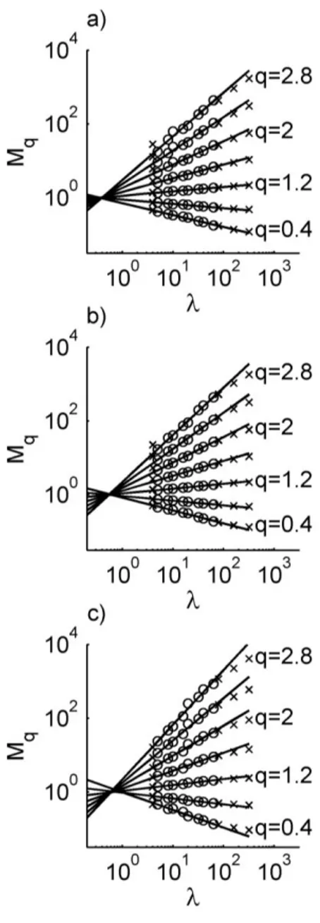
The empirical scaling analysis described above is applied to surface accumulated precipitation spatial fields over 5 hour simulations, . Here the constant value domain length) was used for the cascade outer scale, . Changing the chosen value of has no effect on the estimated value of the slope of the fitted lines, i.e. on and respective UM parameter estimation. Fig. 2.3a-c shows log-log plots of against for fields for three different simulations. The lines are only fitted to the range of scales that are well resolved by the model, i.e. larger than and smaller than about . For the linear fits are good implying that statistical scale invariance predicted by Eq. 2.4 is a good

(39)

representation, and that there are no characteristic scales or scale breaks for the considered ranges of and (from ~1 to ~ 20 km). This range of is similar to the ones found in literature for similar analysis (e.g Douglas and Barros, 2003; Lovejoy et al., 2008a,b; Nykanen, 2008; de Lima and de Lima, 2009). Some simulations show ersistent deviations from linear behavior at particular scales, but the relation between these scales and varies between simulations, suggesting that the small-scale terrain wavelength is not (statistically) a characteristic scale in the rain fields. The same spatial scaling analysis was repeated for the fields resulting from all simulations in Table 2.1, all of them showing the same robust scaling behavior (linear relations).

Figure 2.3. Relationship between and for different values of q. is computed from from simulation a) Sst5km, b) Sst10km, c) Sst15km. The scales considered on the analysis are ark by ‘o’ whi ‘x’ arks th ones not considered. The plots are on a log-log scale.

(40)

Figure 2.4. The scaling exponent function, for a) varying , b) varying with and c) varying with . The empirical estimated is showed with markers and the UM model fit is represented by full line.

The scaling exponent function, , and respective UM parameters can be used to quantify the multifractal behavior. Fig. 2.4 shows that for q<2 there is a very robust match between empirically estimated scaling exponent function, , (i.e. slopes of the fitted lines in log-log plots of against ) from fields for the different simulations and the UM model curves (solid lines), computed from Eq. 2.5 with the UM parameters obtained from DTM technique, which is consistent with the literature (e.g. Nykanen, 2008; Lovejoy et al. (2008a), Stolle, 2009, among others). It is also important to notice the variation of with varying simulation