J. Braz. Soc. Mech. Sci. & Eng. vol.30 número2

(1)

!" ##$ % &' &

(###

' )

' * !!# # # % &' &

The present paper deals with the determination of thermal stresses in a thick circular plate under steady temperature field. A thick circular plate is considered having constant initial temperature and arbitrary heat flux is applied on the upper face with lower face at initial temperature and the fixed circular edge is thermally insulated. Heat is exchanged through heat transfer at lower boundary surface. The results are obtained in series form in terms of Bessel’s functions and they are illustrated numerically.

Keywords: quasi-static, steady state, thermoelastic problem, thermal stresses

Introduction

1

During the second half of the twentieth century, nonisothermal problems of the theory of elasticity became increasingly important. This is due to their wide application in diverse fields. The high velocities of modern aircraft give rise to aerodynamic heating, which produces intense thermal stresses that reduce the strength of the aircraft structure.

Nowacki (1957) has determined steady-state thermal stresses in circular plate subjected to an axisymmetric temperature distribution on the upper face with zero temperature on the lower face and the circular edge. Roy Choudhary (1972) (1973) and Wankhede (1982) determined Quasi-static thermal stresses in thin circular plate. Gogulwar and Deshmukh (2005) determined thermal stresses in thin circular plate with heat sources. Also Tikhe and Deshmukh (2005) studied transient thermoelastic deformation in a thin circular plate, where as Qian and Batra (2004) studied transient thermoelastic deformation of thick functionally graded plate. Moreover, Sharma et al (2004) studied the behavior of thermoelastic thick plate under lateral loads and obtained the results for radial and axial displacements and temperature change have been computed numerically and illustrated graphically for different theories of generalized thermoelasticity. Also Nasser M.EI-Maghray (2004) (2005) solved two-dimensional problem of thick plate with heat sources in generalized thermoelasticity. Recently Ruhi et al (2005) did thermoelastic analysis of thick walled finite length cylinders of functionally graded materials and obtained the results for stress, strain and displacement components through the thickness and along the length are presented due to uniform internal pressure and thermal loading.

The present paper deals with the determination of thermal stresses in a thick circular plate under steady temperature field. A thick circular plate is considered having constant initial temperature and arbitrary heat flux is applied on the upper face with lower face at initial temperature and the fixed circular edge is thermally insulated. Heat is exchanged through heat transfer at lower boundary surface.

This paper contains, new and novel contribution of thermal stresses in quasi-static thick plate under steady state. The results presented here will be more useful in engineering problem particularly in the determination of the state of strain in thick circular plate constituting foundations of containers for hot gases or liquids, in the foundations for furnaces etc.

Paper accepted February, 2008. Technical Editor: Nestor A. Zouain Pereira.

Formulation of the Problem

Consider a thick circular plate of radius a and thickness h defined by 0≤r≤a,−h/2≤z≤h/2. The initial temperature in a thick circular plate is given by constant T_i. The heat flux

( )

/λ 0f r Q

− is applied on the upper surface of plate

(

z=h/2

)

and lower face

(

z=−h/2

)

is at initial temperatureTi. The fixed circular edge

(

r=a

)

is thermally insulated. Under these more realistic prescribed conditions, the steady state thermal stresses are required to be determined.

The differential equation governing the displacement potential function

φ

( )

r,z is given in Noda et al (2003) as

τ

φ

_K

z r r

r ∂ =

∂ + ∂ ∂ + ∂ ∂

2 2

2 2 ₁

(1)

where K is the restraint coefficient and temperature change i

T T− =

τ ,T_i is initial temperature. Displacement function φ is known as Goodier’s thermoelastic displacement potential.

The steady state temperature of the plate satisfies the heat conduction equation,

0 1

2 2

= ∂ ∂ + ∂ ∂ + ∂ ∂

z T r T r r

T

(2)

with the boundary conditions

) r ( Qof z T

− = ∂ ∂

λ atz=h/2,0≤r≤a (3)

i T

T = atz=−h/2,0≤r≤a (4)

0 = ∂ ∂ r T

at r=a,−h/2≤z≤h/2 (5)

and

i T

T = at t = 0 (6)

(2)

J. of the Braz. Soc. of Mech. Sci. & Eng. Copyright  2008 by ABCM April-June 2008, Vol. XXX, No. 2 / 175 rdz

M r u_r

∂ ∂ − ∂ ∂

= φ 2 (7)

2 2 2 1 2

z M M ) ( z u_z

∂ ∂ − ∇ − + ∂ ∂

= φ ν (8)

The Michell’s function M must satisfy

0 2 2_∇ ₌

∇ M (9)

where

2 2

2 1

z r . r

r ∂

∂ + ∂

∂ =

∇ (10)

The component of the stresses are represented by the thermoelastic displacement potential

φ

and Michell’s function M as

   

   

    

  

∂ ∂ − ∇ ∂

∂ + − ∂ ∂ =

2 2 2 2

2 2

r M M v z K r G

rr φ τ

σ (11)

   

 

   

 

∂ ∂ − ∇ ∂

∂ + − ∂ ∂ =

r M r M v z K r r

G 1 1

2 φ τ 2

σθθ (12)

   

   

    

  

∂ ∂ − ∇ − ∂

∂ + − ∂ ∂ =

2 2 2 2

2

2 2

z M M ) v ( z K z G

zz φ τ

σ (13)

and

   

   

    

  

∂ ∂ − ∇ − ∂

∂ + ∂ ∂ ∂

=₂ 2 ₁ 2 2₂

z M M ) v ( r z r G rz

φ

σ (14)

where G and

ν

are the shear modulus and Poisson’s ratio respectively,

For traction free surface stress functions

0 = = rz

rr σ

σ at r=a 0 = = rz

zz σ

σ at

2 h

z=± (15)

Equation (1) to (15) constitutes mathematical formulation of the problem.

Solution

To obtain the expression for temperature T(r, z):

Assume

∑

∞

= 

 

 

     

+ +

= 1

0

2 sinh

) ( )

, (

n

n n

n i

h z r

J A T

z r

T α α (16)

where α₁,α₂_,...are roots of the transcendental equation

( )

0

1 ⋅a =

J α . where Jn

( )

x is Bessel function of the first kind of order n and Anis constant. The constant An can be found from the nature of temperature on upper face.

Using equations (3), (16) and by theory of Bessel’s function one obtains

∫

−

= a n

n n

n

n rJ r f r dr

h a

J a

Qo A

0 0 2

0

2 ₍ ₎_cosh( ₎ ( ) ( )

2

α α

α

λα (17)

equations (16) and (17) gives the required expression for steady state temperature function.

The temperature change

τ

is obtained by using

i T T− =

τ

Hence

∑

∞

= 

 

 

     

+ =

1 0

2 sinh

) ( )

, (

n

n n

n

h z r

J A z

r α α

τ (18)

Now suitable form of M satisfying (9) is given by

∑

∞

= 

  

   

 

     

+ =

1 0

2 cosh

) ( n

n n n

h z B

r J

M α α

       

 

     

+ 

    

+ +

2 sinh

2

C_nα_n z h α_n z h (19)

where B_n and C_nare arbitrary functions. Assuming displacement function φ

( )

r,z as

∑

∞

= 

 

 

     

+ 

    

+ =

1 0

2 cosh

) ( 2

) , , (

n

n n

n

h z r

J D h z t z

r α α

φ (20)

Using

φ

in (1), one have

n n KA Dn

α

2 =

Thus equation (20) become

∑

∞

= 

 

 

     

+ 

    

+ =

1 0

2 cosh

) ( 2

2 ) , (

n

n n

n

nJ r _z h

A h z K z

r α

α α

φ (21)

Now using equations (18) (19) and (21) in (7) (8) and (11) to (14), one obtains the expressions for displacements and stresses respectively as

   

 

     

+ 

    

+ 

  

     − =

∑

∞

=₁ 1( ) 2 2 cosh 2

h z h

z KA r J

u n

n

n n

r α α

   

 

     

+ +

2 sinh

2 h

z B_nα_n α_n

     

+ +    

 

     

+ +

2 2

sinh

2 h

z h

z

Cnαn αn αn

       

 

     

+ ×

2

(3)

            +             =

∑

∞

=₁ 0( ) 2 cosh 2

h z KA r J u n n n n n z α α α             +       + + 2 sinh 2 h z h z _n n α α             + − 2 cosh 2 h z Bnαn αn

            + − + 2 cosh ) 2 1 ( 2 2 h z v

Cnαn αn

                +       + − 2 sinh 2 h z h z _n n α α (23)           −      − =

∑

∞ =1 1 0 ) ( ) ( 2 2 n n n n n rr r r J r J A K

G α α α

σ             +       + × 2 cosh 2 h z h

z α_n

            + −

∑

∞

=₁ 0( ) sinh 2

h z r J A K _n n n

n α α

            +       − +

∑

∞

= sinh 2

) ( ) ( 1 1 0

2 _z h

r r J r J B n n n n n n n α α α α α

∑

∞ =            + + 1 0 2 2 sinh ) ( 2 n n n n n n h z r vJ

C α α α α

                +       − + 2 sinh ) ( ) ( 1 0 h z r r J r

J n n n

n α α α α                     +       + + 2 cosh 2 h z h z n n α α (24)             +       +          − =

∑

∞

= 2 cosh 2

) ( 2

2

1

1 _z h _z h

r r J A K G n n n

n α _α

σθθ             + −

∑

∞

=₁ 0( )sinh 2

h z r J A K n n n

n α α

∑

∞ =            + + 1 1 2 2 sinh ) ( n n n n n h z r r J

B α α α

∑

∞ =

























+

1 0 2

2 sinh

)

(

2

n n n n n n

h

z

r

vJ

C

α

                +       + 2 sinh ) (

1 _z h

r r J n n _α α                     + ×       + + 2 cosh 2 h z h z n n α α (25)                 +       =

∑

∞ =1 0 2 sinh 2 ) ( 2 2 n n n n zz h z r J A K

G α α

σ             +       + + 2 cosh 2 h z h

z αn

∑

∞ =            + − 1 0 2 sinh ) ( n n n n h z r J A

K α α

∑

∞ =            + − 1 0 3 2 sinh ) ( n n n n n h z r J

Bα α α

∑

∞ =            +       + + 1 0 3 2 cosh 2 ) ( n n n n n h z h z r J

C α α α

                +       + − 2 cosh 2 h z h z n n α α (26)                 +      ₋ =

∑

2 cosh ) ( 2

2G K A_nJ₁ _nr _n z h

rz α α

σ             +       + + 2 sinh 2 h z h z n n α α

∑

∞ =            + + 1 1 3 2 cosh ) ( n n n n n h z r J

Bα α α

            + +

∑

∞

=₁ 1( ) 2 cosh 2

3 _J _r _v _z h

C _n

n

n n

nα α α

                +       + + 2 sinh 2 h z h z n n α α (27)

Now in order to satisfy equation (15) solving equation (24) to (27) for

B

_nand

C

_n one obtain

(

)

3 2 2 1 n n n KA B α ν −

= (28)

3 2 n n n KA C α = (29)

Using these values of

B

_n and

C

_nin equations (22) to (27) one obtain the expressions for displacements and stresses as

( )

∑

∞ =            + − = 1 1 2 sinh ) ( 1 n n n n n r h z r J A K

u α α

α ν (30)

( )

            + − =

∑

∞ = 2 cosh ) ( 1 1 0 h z r J A K u _n n n n n

z ν _α α α (31)

( )

            +       − − =

∑

∞

= sinh 2

) ( 1

2

1

1 _z h

r r J A GK n n n n n

rr _α α

α ν σ (32)

( )

∑

∞ =      − − = 1 0 1 ) ( ) ( 1 2 n n n n

n J r

r r J A GK α α α ν σθθ             + × 2

sinhαn z h (33)

0 = zz σ (34) 0 = rz

(4)

J. of the Braz. Soc. of Mech. Sci. & Eng. Copyright  2008 by ABCM April-June 2008, Vol. XXX, No. 2 / 177

Numerical Calculation

Setting f(r)=Ti+Toδ(r−b) (a > b) at 2 h

z= , (36)

in equation (17), where

T

₀is constant and b<a, one has

) cosh( ) (

) ( 2

2 0 2

0 0 0

h a

J a

b J bQ T A

n n

n

n n

α α

λα

α

−

=  (37)

The numerical calculation have been carried out for steel (SN 500) plate with parameters a=1m,b=0.5m,h=0.5m, thermal diffusivity _k₌_15.9_×₁₀−6

( )

_m2_s−1 _a_nd_{Poisson ratio}ν ₌₀_.₂₈₁ _with

, 8317 . 3 1=

α α₂=7.0156, α₃=10.1735, α₄=13.3237, ,

470 . 16 5=

α α6 =19.6159, α7=22.7601, α8=25.9037, ,

0468 . 29 9 =

α α10=32.18 are the roots of transcendental equation J1(αa)=0.

For convenience setting

λ ν λ

ν

2 2

) 1 ( 4 , ) 1 ( 2

a

GK TobQo

B a

K TobQo

A=− − = − in the expressions

(16) and (30) to (35). The numerical expressions for temperature, displacement and stress components are obtained as

∑

∞

= 



    −

=

1 02 0 0

2 ₍ ₎_cosh( ₎

) ( ) ( 2

n n n n

n n i

h a

J

b J r J a

TobQo T

T

α α

α

α α λ

   

 

     

+ ×

2

sinhαn z h (38)

∑

∞

= 

 

 

     

+ 

  

    =

1 2 02 0 1

2 sinh

) cosh( ) (

) ( ) ( n

n n

r _z h

h a

J

b J r J A

u _α

α α

α

α α

(39)

   

 

     

+ 

  

    =

∑

∞

= 2

cosh ) cosh( ) (

) ( ) ( 1 02

0

0 _z h

h a

J

b J r J A

u

n

n n n n

n n

z _α

α α

α

α α

(40)

   

 

     

+ 

  

    =

∑

∞

= 2

sinh ) cosh( ) (

) ( ) ( 1 2 02

0

1 _z h

h a

J r

b J r J

B _n _n _n _n n

n n

rr _α

α α

α

α α

σ

(41)

∑

∞

= 

  

    =

1 02 0

) cosh( ) (

) (

n n n n

n h a

J

b J

B _α _α _α

α σθθ

   

 

     

+ 

  

 

− ×

2 sinh

) ( )

( 1

0

h z r

r J r

J _n

n n

n _α α

α

α (42)

0 = = rz

zz σ

σ (43)

In order to examine the influence of steady state temperature field on the thick plate, one performed the numerical calculationsr=0,0.2,0.4,0.6,0.8,1and

25 . 0 , 125 . 0 , 0 , 125 . 0 , 25 .

0 −

− =

z Numerical variations in radial and

axial directions are shown in the figures with the help of computer programme.

-0,02 0 0,02 0,04 0,06 0,08 0,1

0 0,2 0,4 0,6 0,8 1

r

Figure1. The radial displacement function u_r/A in radial direction.

-0.02 0 0.02 0.04 0.06 0.08 0.1

-0.3 -0.2 -0.1 0 0.1 0.2 0.3

Z

Figure 2. The radial displacement function u_r/Ain axial direction.

-0.08 -0.06 -0.04 -0.02 0 0.02 0.04 0.06 0.08 0.1

0 0.2 0.4 0.6 0.8 1

r

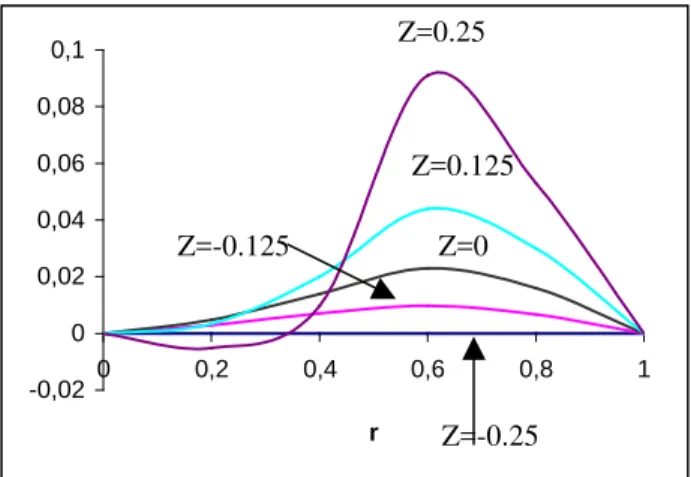
Figure 3. The axial displacement function u_z/A in radial direction. Z=0.25

Z=0 Z=-0.125

Z=-0.25 Z=0.125

r= 0.4 r = 0.8 r =0.6

r= 0 & r= 1

r= 0.2

z= -0.125 & -0.25

z= 0 z= 0125

(5)

-0.08 -0.06 -0.04 -0.02 0 0.02 0.04 0.06 0.08 0.1

-0.3 -0.2 -0.1 0 0.1 0.2 0.3

z

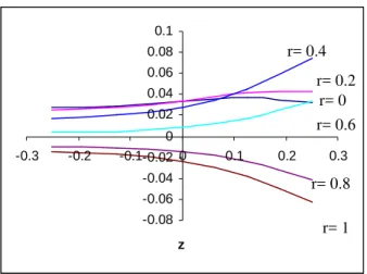
Figure 4. The axial displacement function u_z/AI n axial direction.

-0.04 -0.02 0 0.02 0.04 0.06 0.08 0.1 0.12 0.14 0.16 0.18

0 0.2 0.4 0.6 0.8 1

r

F

Figure 5. The radial stress function σ_rr/B in radial direction.

-0,05 0 0,05 0,1 0,15 0,2

-0,3 -0,2 -0,1 0 0,1 0,2 0,3

z

r =0 & r =1

Figure 6. The radial stress function σ_rr/B in axial direction.

-0,4 -0,3 -0,2 -0,1 0 0,1 0,2 0,3

0 0,2 0,4 0,6 0,8 1

r

Figure7. The stress function σθθ/B in radial direction.

-0,4 -0,3 -0,2 -0,1 0 0,1 0,2 0,3

-0,3 -0,2 -0,1 0 0,1 0,2 0,3

z

Figure 8. The stress function σθθ/B in axial direction.

Concluding Remarks

In this paper a thick circular plate is considered which is free from traction and determined the expressions for temperature, displacement and stress function due to steady state temperature field. As a special case mathematical model is constructed for

) ( )

(r T To r b

f = i+ δ − (a > b) at 2 h z=

and performed numerical calculations. The thermoelastic behavior is examined such as temperature, displacement and stresses with the help of arbitrary heat flux is applied on the upper surface.

From figure 1 and 2, radial displacement function

u

_r is zero at r=0,r=1and

z

=−0.25Also it can observe that it shows variation on upper half of plate within annular region

1 4 .

0 ≤

r

≤ and decreases in the direction of lower surface.

From figure 3 and 4, axial displacement function

u

_z shows variation on upper half of plate within circular region 0≤

r

≤1and decreases in the direction of lower surface.

From figure 5 and 6, stress function

σ

_rr is zero atr=0,r=1and

z

=−0.25. Also it can observe that it shows variation on upper half of plate within circular region 0≤

r

≤1 and decreases in the direction of lower surface.

r= 1 r= 0.8 r= 0 r= 0.2

r= 0.6 r= 0.4

z= 0.125

z= 0 z=-0.125

z=-0.25 z= 0.25

r= 0.4 r= 0.8

r= 0.2 r= 0.6

z= 0.25

z= 0.125

z= 0

z= -0.125

z= 0.25

r= 0.8 & 1 r= 0.2 &0.6

(6)

J. of the Braz. Soc. of Mech. Sci. & Eng. Copyright  2008 by ABCM April-June 2008, Vol. XXX, No. 2 / 179

From figure 7 and 8, the stress function

σ

_θθ shows variation on upper half of plate within circular region 0≤

r

≤1 and decreases in the direction of lower surface.

It means we may find out that displacement and stress components occurs near heat source. Radial stress component

σ

_rr develops tensile stress near heat source and compressive stress out of the heat source, where as stress component

σ

_θθ develops compressive stress near heat source and tensile stress out of heat source. Also axial stress component

σ

_zz and resultant stress component

σ

_rz are zero due to exchange of heat through heat transfer in axial direction (i.e. from upper surface to lower surface).

From figures of radial and axial displacements it can observe that the radial displacement occur away from the center

(

r=0

)

where as axial displacement is maximum at upper surface near heat source. So it may conclude that due to heat flux applied on upper surface of plate under steady state, the plate bends concavely at the heat source i.e.

(

r=0.5

)

.

The results obtained here are more useful in engineering problems particularly in the determination of state of strain in thick circular plate. Also any particular case of special interest can be derived by assigning suitable values to the parameters and function in the expression (30) - (35).

Acknowledgement

The authors are thankful to University Grants Commission, New Delhi to provide the partial financial assistance under major research project scheme.

References

Gogulwar, V.S. and Deshmukh, K.C., 2005, “Thermal stresses in a thin circular plate with heat sources”, Journal of Indian Academy of Mathematics, Vol .27, No. 1, 2005.

Nasser M.EI-Maghraby, 2004, “Two dimensional problem with heat sources in generalized thermoelasticity with heat sources”, Journal of Thermal Stresses, Vol. 27, pp. 227-239.

Nasser M.EI-Maghraby, 2005, “Two dimensional problem for a thick plate with heat sources in generalized thermoelasticity”, Journal of Thermal Stresses, Vol. 28, pp. 1227-1241.

Noda, N.; Hetnarski, R. B. and Tanigawa, Y., 2003, “Thermal Stresses”, 2nd_{ed., pp 259-261, Taylor and Francis, New York.}

Nowacki, W., 1957, “The state of stresses in a thick circular plate due to temperature field”, Bull. Acad. Polon. Sci., Scr. Scl. Tech., Vol.5, pp 227.

Qian, L. F., and Batra, R. C., 2004, “Transient thermoelastic deformation of a thick functionally graded plate”, Journal of Thermal Stresses, Vol. 27, pp. 705-740.

Roy Choudhary, S.K., 1972, “A note of Quasi static stress in a thin circular plate due to transient temperature applied along the circumference of a circle over the upper face”, Bull Acad. Polon Sci, Ser, Scl, Tech, pp 20-21. Roy Choudhary, S.K., 1973, “A note on Quasi-static thermal deflection of a thin clamped circular plate due to ramp-type heating of a concentric circular region of the upper face”, Journal of the Franklin Institute, Vol .206, No 3, Sept.

Ruhi, M.; Angoshatari, A. and Naghdabadi, R., 2005, “Thermoelastic analysis of thick walled finite length cylinders of functionally graded material”, Journal of Thermal Stresses, Vol. 28, pp. 391-408.

Sharma, J. N.; Sharma, P. K. and Sharma, R. L., 2004, “Behavior of thermoelastic thick plate under lateral loads”, Journal of Thermal Stresses, Vol. 27, pp. 171-191.

Tikhe, A. K. and Deshmukh, K. C., 2005, “Transient thermoelastic deformation in a thin circular plate”, Journal of Advances in Mathematical Sciences and Applications, Vol. 15, No. 1.