CryoSat-2 delivers monthly and inter-annual surface elevation change for Arctic ice caps

(1)

TCD

9, 2821–2865, 2015

CryoSat-2 delivers monthly and inter-annual surface elevation change for

Arctic ice caps

L. Gray et al.

Title Page

Abstract Introduction

Conclusions References

Tables Figures

◭ ◮

Back Close

Full Screen / Esc

Printer-friendly Version

Interactive Discussion

Discussion

P

a

per

|

Discussion

P

a

per

|

Discussion

P

a

per

|

Discussion

P

a

per

|

The Cryosphere Discuss., 9, 2821–2865, 2015 www.the-cryosphere-discuss.net/9/2821/2015/ doi:10.5194/tcd-9-2821-2015

This discussion paper is/has been under review for the journal The Cryosphere (TC). Please refer to the corresponding final paper in TC if available.

CryoSat-2 delivers monthly and

inter-annual surface elevation change for

Arctic ice caps

L. Gray1, D. Burgess2, L. Copland1, M. N. Demuth2, T. Dunse3, K. Langley3, and T. V. Schuler3

1

Department of Geography, University of Ottawa, Ottawa, K1N 6N5, Canada

2

Natural Resources Canada, Ottawa, Canada

3

Department of Geosciences, University of Oslo, Oslo, Norway

Received: 29 April 2015 – Accepted: 29 April 2015 – Published: 26 May 2015

Correspondence to: L. Gray (laurence.gray@sympatico.ca)

(2)

TCD

9, 2821–2865, 2015

Arctic ice caps

L. Gray et al.

Title Page

Tables Figures

◭ ◮

Back Close

Full Screen / Esc

Discussion

P

a

per

|

Discussion

P

a

per

|

Discussion

P

a

per

|

Discussion

P

a

per

|

Abstract

We show that the CryoSat-2 radar altimeter can provide useful estimates of surface elevation change on a variety of Arctic ice caps, on both monthly and yearly time scales. Changing conditions, however, can lead to a varying bias between the eleva-tion estimated from the radar altimeter and the physical surface due to changes in the

5

contribution of subsurface to surface backscatter. Under melting conditions the radar returns are predominantly from the surface so that if surface melt is extensive across the ice cap estimates of summer elevation loss can be made with the frequent cov-erage provided by CryoSat-2. For example, the avcov-erage summer elevation decreases on the Barnes Ice Cap, Baffin Island, Canada were 2.05±0.36 m (2011), 2.55±0.32 m

10

(2012), 1.38_±0.40 m (2013) and 1.44_±0.37 m (2014), losses which were not balanced by the winter snow accumulation. As winter-to-winter conditions were similar, the net elevation losses were 1.0±0.2 m (winter 2010/2011 to winter 2011/2012), 1.39±0.2 m

(2011/2012 to 2012/2013) and 0.36_±0.2 m (2012/2013 to 2013/2014); for a total sur-face elevation loss of 2.75±0.2 m over this 3 year period. In contrast, the uncertainty

15

in height change results from Devon Ice Cap, Canada, and Austfonna, Svalbard, can be up to twice as large because of the presence of firn and the possibility of a varying bias between the true surface and the detected elevation due to changing year-to-year conditions. Nevertheless, the surface elevation change estimates from CryoSat for both ice caps are consistent with field and meteorological measurements. For example, the

20

average 3 year elevation difference for footprints within 100 m of a repeated surface GPS track on Austfonna differed from the GPS change by 0.18 m.

1 Introduction

Recent evidence suggests that mass losses from ice caps and glaciers will contribute significantly to sea level rise in the coming decades (Meier et al., 2007; Gardner et al.,

25

(3)

TCD

9, 2821–2865, 2015

Arctic ice caps

L. Gray et al.

Title Page

Tables Figures

◭ ◮

Back Close

Full Screen / Esc

Discussion

P

a

per

|

Discussion

P

a

per

|

Discussion

P

a

per

|

Discussion

P

a

per

|

ice caps are very limited: satellite techniques, such as repeat gravimetry from GRACE (Gravity Recovery and Climate Experiment), favour the large Greenland or Antarctic Ice Sheets, while surface and airborne experiments sample conditions sparsely in both time and space. Satellite laser altimetry (ICESat) was used between 2003 and 2009 but the results were limited by both laser lifetime and atmospheric conditions. NASA’s

5

follow-on mission (ICESat 2, Abdalati et al., 2010) is currently scheduled for launch in 2017, but until then CryoSat-2 (CS2), launched by the European Space Agency (ESA) in 2010, provides the only high resolution satellite altimeter able to routinely measure small ice caps and glaciers. The new interferometric (SARIn) mode of CS2 (Wingham et al., 2006) has important new attributes in comparison to previous satellite

10

radar altimeters: Delay-Doppler processing (Raney, 1998) permits a relatively small (∼380 m) along-track resolution (Bouzinac, 2014), while the cross-track interferometry

(Jensen, 1999) provides information on the position of the footprint centre. Here we show that the SARIn mode of CS2 can measure annual height change of smaller Arctic ice caps, and even provide estimates of summer melt on a monthly time frame.

15

To test and validate the CS2 altimeter, ESA developed the airborne ASIRAS Ku-band (13.5 GHz) radar altimeter. ASIRAS has been operated during field campaigns under the CryoSat Validation Experiment (CryoVex) at selected sites before and after the launch of the satellite. One of the most interesting revelations of the ASIRAS data has been the demonstration of variability in relative surface and subsurface returns in

20

a variety of locations including Devon Ice Cap in Canada, Greenland and Austfonna in Svalbard (Hawley et al., 2006, 2013; Helm et al., 2007; Brandt et al., 2008; de la Pena et al., 2010). The time variation of the ASIRAS return signals from the surface and near surface (the “waveforms”) can and does vary significantly from year-to-year at the same geographic position, and in any one year with changing position across

25

(4)

TCD

9, 2821–2865, 2015

Arctic ice caps

L. Gray et al.

Title Page

Tables Figures

◭ ◮

Back Close

Full Screen / Esc

Discussion

P

a

per

|

Discussion

P

a

per

|

Discussion

P

a

per

|

Discussion

P

a

per

|

characteristics, dependent on past meteorological conditions, could therefore affect the relative strength of the surface and volume component of the CS2 return signal and affect the bias between the elevation measured by CS2 and the true surface.

In this study we use all available SARIn data from July 2010 to December 2014 to undertake the first systematic measurement by spaceborne radar of elevation change

5

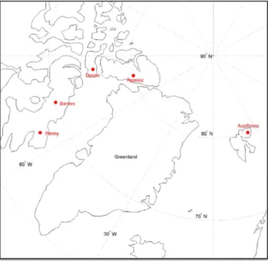
on a variety of ice caps across the Canadian and Norwegian Arctic (Fig. 1) representing a wide range of climate regimes. Emphasis is placed on CS2 results from Devon and Austfonna as both ice caps were selected by ESA as designated calibration/validation sites, and a wide range of ground and airborne validation datasets are available. SARIn data are also used to measure height changes on Penny, Agassiz and Barnes ice

10

caps to illustrate the wide applicability of the method in areas where there is less data available for surface validation. Together with the recent CS2 work on Greenland and Antarctica (McMillan et al., 2014a; Helm et al., 2014), this illustrates the power of the new interferometric mode of the CS2 altimeter to provide useful information in an all-weather, day-night situation.

15

Our emphasis in this paper is to demonstrate that CS2 can measure elevation and elevation change on relatively small ice caps, even with di_ffering surface conditions, and for some on a monthly time scale. The many complications associated with converting the CS2 elevation change data to an ice cap wide mass balance will be treated in future papers.

20

2 Study areas

We begin by describing the two ice caps, Devon and Austfonna, which were part of the CryoVex campaigns and which have a wide range of surface reference data. Then we discuss conditions on Barnes, Agassiz and Penny ice caps. Although these ice caps have less surface reference data, they are quite different and represent a good test of

25

(5)

TCD

9, 2821–2865, 2015

Arctic ice caps

L. Gray et al.

Title Page

Tables Figures

◭ ◮

Back Close

Full Screen / Esc

Discussion

P

a

per

|

Discussion

P

a

per

|

Discussion

P

a

per

|

Discussion

P

a

per

|

2.1 The Devon Ice Cap

Occupying_∼12 000 km2of eastern Devon Island, Nunavut, the main portion of the De-von Ice Cap (75◦N, 82◦W) ranges from sea-level, where most outlet glaciers terminate, to the ice cap summit at∼1920 m. While the ice cap loses some mass through iceberg

calving (Burgess et al., 2005; Van Wychen et al., 2012), the main form of ablation is

5

through runoff, which is controlled primarily by the intensity and duration of summer melt (Koerner, 1966, 2005). Surface accumulation is asymmetric and can be as much as twice as high in the south-east compared to the north-west due to the proximity to Baffin Bay (Koerner, 1966). Surface mass balance has been negative across the Northwest sector since 1960 (Koerner, 2005), but after 2005 the surface melt rates

10

have been_∼4 times greater than the long-term average (Sharp et al., 2011). This has led to a thinning of∼6 m of the northwest basin since the sixties (Burgess, 2014). The

ice cap is characterized by four glacier-facies zones that have developed at various al-titudes as a function of prevailing climatic conditions (Koerner, 1970): below_∼1000 m annual melting removes all winter precipitation, creating the “ablation” zone. Above this

15

(∼1000–1200 m), the “superimposed ice” zone develops, where refreezing of surface

melt results in a net annual mass gain. In the “wet snow” zone (_∼1200–1400 m) the winter snowpack experiences sufficient melt during the summer that meltwater perco-lates into one or more previous year’s firn layers. The highest “percolation” zone typ-ically occupies elevations above_∼1400 m to the ice cap summit, where surface melt

20

is refrozen within the winter snowpack. It is important to emphasize that the distribu-tion of these facies varies year-to-year, reflecting meteorological condidistribu-tions and mass balance history.

2.2 Austfonna

Occupying∼8100 km2of Nordaustlandet, Svalbard, Austfonna (79◦N, 23◦E) is among

25

(6)

TCD

9, 2821–2865, 2015

Arctic ice caps

L. Gray et al.

Title Page

Tables Figures

◭ ◮

Back Close

Full Screen / Esc

Discussion

P

a

per

|

Discussion

P

a

per

|

Discussion

P

a

per

|

Discussion

P

a

per

|

basins form a continuous calving front towards the Barents Sea, while the north-western basins terminate on land or in narrow fjords (Dowdeswell et al., 1986a). Sev-eral drainage basins are known to have surged in the past (Dowdeswell et al., 1986b), including Basin-3 which entered renewed surge activity in autumn 2012 (McMillan et al., 2014b; Dunse et al., 2015).

5

Mass balance stakes indicate an equilibrium line altitude (ELA) of ∼450 m in the

NE and∼250 m in the SE of Austfonna (Moholdt et al., 2010). This reflects a typical

asymmetry in snow accumulation with the southeastern slopes receiving about twice as much precipitation as the northwestern slopes, as the Barents Sea to the east rep-resents the primary moisture source (Pinglot et al., 2001; Taurisano et al., 2007; Dunse

10

et al., 2009).

Despite a surface mass balance close to zero (2002–2008), the net mass balance of Austfonna has been negative at−1.3±0.5 Gt a−1(Moholdt et al., 2010), due to calving

and retreat of the marine ice margin (Dowdeswell et al., 2008). Sporadic glacier surges, as currently seen in Basin-3 (McMillan et al., 2014; Dunse et al., 2015) can significantly

15

alter the calving flux from the ice cap. Prior to the surge of Basin-3, interior thickening at rates of∼0.5 m a−1and marginal thinning of 1–3 m a−1had been detected from repeat

airborne (1996–2002; Bamber et al., 2004) and satellite laser altimetry (2003–2008; Moholdt et al., 2010). The accumulation area comprises an extensive superimposed ice and wet snow zone, and in some years a percolation zone may exist. The distribution of

20

glacier facies varies significantly from year to year, a consequence of large inter-annual variability in total amount of snow and summer ablation (Dunse et al., 2009). Despite mean annual temperatures of−8.3◦C, large temperature variations occur throughout

the year and it is not uncommon for temperatures above 0◦_{C and rain events to occur} in winter (Schuler et al., 2014).

25

2.3 Barnes Ice Cap

Barnes Ice Cap (70◦_{N, 73}◦_{W) is a near-stagnant ice mass that occupies}

∼5900 km2

(7)

TCD

9, 2821–2865, 2015

Arctic ice caps

L. Gray et al.

Title Page

Tables Figures

◭ ◮

Back Close

Full Screen / Esc

Discussion

P

a

per

|

Discussion

P

a

per

|

Discussion

P

a

per

|

Discussion

P

a

per

|

most of its perimeter, and its surface rises gradually towards the interior, reaching a maximum elevation of_∼1100 m along the summit ridge (Andrews and Barnett, 1979). In-situ surface mass balance measurements (1970–1984), indicate winter accumula-tion rates of∼0.5 m snow water equivalent (s.w.e.), and net balance for the entire ice

cap of₋0.12 m a−1_{(Sneed et al., 2008). Mean mass loss rates have become}

increas-5

ingly negative (−1.0±0.14 m a−1) up to the present (Abdalati et al., 2004; Sneed et al.,

2008; Gardner et al., 2012). In the past accumulation occurred primarily as superim-posed ice (Baird, 1952), but more recently summer melt has been extensive and the ice cap has lost its entire accumulation area (Dupont et al., 2012). Similar to glaciers in the Queen Elizabeth Islands (Koerner, 2005), the surface mass balance of the Barnes

10

Ice Cap is driven almost entirely by the magnitude and duration of summer melt (Sneed et al., 2008).

2.4 Agassiz Ice Cap

Agassiz Ice Cap (80◦N, 75◦W) occupies∼21 000 km2of the Arctic Cordillera on

north-eastern Ellesmere Island. It ranges in elevation from sea-level, where several of the

15

major tidewater glaciers that drain the ice cap interior terminate, to ∼1980 m at the

central summit. Ice core records acquired from the summit region indicate that melt rates since the early 1990’s are comparable to those last experienced in the early Holocene∼9000 years ago (Fisher et al., 2012). In-situ measurements of surface mass

balance indicate a long term ELA of ∼1100 m with an average accumulation rate of

20

0.13 m w.e. over the period 1977–present. Between the summit and the sea level outlet glaciers there is a progression of ice facies similar to that described for Devon.

Repeat airborne laser altimetry surveys conducted in 1995 and 2000 indicate zero change to slight thickening at high elevations, but the ice loss at lower elevations led to an estimate of ice cap wide thinning of _∼0.07 m a−1 _{(Abdalati et al., 2004). More}

25

(8)

TCD

9, 2821–2865, 2015

Arctic ice caps

L. Gray et al.

Title Page

Tables Figures

◭ ◮

Back Close

Full Screen / Esc

Discussion

P

a

per

|

Discussion

P

a

per

|

Discussion

P

a

per

|

Discussion

P

a

per

|

2.5 Penny Ice Cap

Penny Ice Cap (67◦_{N, 66}◦_{W) occupying}

∼6400 km2of the highland region of southern

Baffin Island, ranges in elevation from 0 to 1980 m and contains one main tidewater glacier, the Coronation Glacier, which calves into Ba_ffin Bay (Zdanowicz et al., 2012). A historical climate record derived from deep and shallow ice cores (Fisher et al., 1998,

5

2012) indicate that current melting on Penny is unprecedented in magnitude and dura-tion for the past∼3000 years. Thickness changes derived from repeat airborne laser

altimetry surveys in 1995 and 2000 indicate an average ice cap wide thinning rate of 0.15 m a−1, with maximum thinning of∼0.5 m a−1in the lower ablation zones (Abdalati

et al., 2004). More recent measurements (2007–2011) indicate thinning of∼3–4 m a−1

10

near the ice cap margin (330 m), amongst the highest rates of glacier melt in the Cana-dian Arctic (Zdanowicz et al., 2012). The current climate regime limits accumulation to elevations above∼1450 m, where it forms as superimposed ice and saturated firn.

Recently, the temperature of the near-surface firn (10 m depth) in the summit region has increased by 10◦C as a result of latent heat release due to increased amounts of

15

summer melt water refreezing at depth (Zdanowicz et al., 2012).

3 Methods

3.1 CS2 SARIn data processing

All available SARIn L1b data files (processed with ESA “baseline B” software; Bouz-inac, 2014) from July 2010 to the end of December 2014 were obtained from ESA for

20

each ice cap. Although developed independently, our processing methodology to derive geocoded heights from the L1b data is similar to that described by Helm et al. (2014), so the summary below focusses on the differences between the two methods.

Delay Doppler processing (Raney, 1998) has been completed in the down-loaded data and the resulting waveform data are included in the ESA L1b files. However,

(9)

TCD

9, 2821–2865, 2015

Arctic ice caps

L. Gray et al.

Title Page

Tables Figures

◭ ◮

Back Close

Full Screen / Esc

Discussion

P

a

per

|

Discussion

P

a

per

|

Discussion

P

a

per

|

Discussion

P

a

per

|

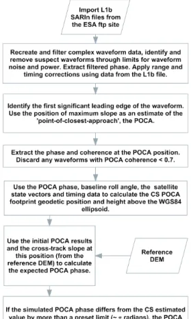
physical results, e.g. terrain footprint height and position, have not been calculated. Our processing for this stage has been developed primarily for the ice cap data ac-quired above, and the steps are illustrated in Fig. 2. The waveform data for each along-track position (time histories of the power, phase and coherence) include the unique “point-of-closest-approach” (POCA) followed in delay time by the sum of surface and

5

subsurface returns from both sides of the POCA (Gray et al., 2013).

An initial examination of the L1b data showed that the received power waveforms varied in both shape and magnitude, and that the peak return did not necessarily fol-low immediately after the first strong leading edge of the return signal. This complexity is not entirely unexpected and arises due to the nature of the surface being

mea-10

sured, in particular the variation in the time history of the illuminated area and the possibility of reflections from sub-surface layers. The problem is then to identify an op-timum algorithm to pick the position of the POCA (the “retracker”) from the waveform. Our approach estimates the POCA position by identifying the maximum slope on the first significant leading edge of the waveform. This is similar to the approach of Helm

15

et al. (2014), who used a particular threshold level on the first significant leading edge of the power waveform.

The choice of the threshold level retracker used by Helm et al. (2014) for their work in Greenland and Antarctica followed that of Davis (1997), who advocated a threshold re-tracker to minimize the dependency of the “retracked” elevation on varying microwave

20

penetration into, and backscattering from, various snow-firn-ice layers. Our tests on the ice caps in our study have shown that a threshold retracker also produces satisfac-tory results but still does not totally eliminate the problem of a variable bias between the detected elevation and the physical surface. In contrast to the interior of Antarctica where near surface melt is very rare, in this study we are dealing with surface and

25

(10)

be-TCD

9, 2821–2865, 2015

Arctic ice caps

L. Gray et al.

Title Page

Tables Figures

◭ ◮

Back Close

Full Screen / Esc

Discussion

P

a

per

|

Discussion

P

a

per

|

Discussion

P

a

per

|

Discussion

P

a

per

|

low in the light of the airborne and CS2 results for particular ice caps, but it is doubtful that an optimum retracker exists for all conditions.

Smoothed phase (Gray et al., 2013; Helm et al., 2014) and information on the in-terferometric baseline are used to estimate the unit vector in the “CryoSat-2 reference frame” (Wingham et al., 2006) pointing towards the POCA in the cross-track swath:

ini-5

tially the phase is used to calculate the look direction with respect to the line connecting the centers of the two receive antennas (the interferometric “baseline”) using the cali-bration provided by Galin et al. (2012). The spacecraft attitude is then used to estimate the look direction to the POCA in the cross-track plane with respect to the nadir direc-tion, perpendicular to the WGS84 ellipsoid. Using the data provided on satellite position

10

and delay times, the latitude, longitude and elevation of the POCA footprints above the WGS84 ellipsoid are then calculated. The results are checked against a reference DEM elevation (Table 1), if the difference is large, typically 50–100 m, then the elevation and position is recalculated with the phase changed by±2πradians. If one of these options corresponds satisfactorily to the reference DEM, and the expected cross-track slope,

15

then the original results are replaced. In this way some of the “blunders” which arise with an ambiguous phase error are avoided. Note the criterion for identifying 2πphase errors and subsequent data replacement depends on the quality of the reference DEM (Table 1).

3.2 Determination of temporal change in surface elevation

20

At the latitude of the Agassiz or Austfonna Ice Caps there is a westward drift of∼15 km

every two days in a sub-satellite track of ascending or descending CS2 orbits, increas-ing to 25, 34 and 38 km at the latitudes of the Devon, Barnes and Penny ice caps respectively (Table 1). The repeat orbit period of CS2 is 369 days, with a 30 day orbit sub-cycle (Wingham et al., 2006). Consequently, the passes over the ice caps tend

25

(11)

TCD

9, 2821–2865, 2015

Arctic ice caps

L. Gray et al.

Title Page

Tables Figures

◭ ◮

Back Close

Full Screen / Esc

Discussion

P

a

per

|

Discussion

P

a

per

|

Discussion

P

a

per

|

Discussion

P

a

per

|

When comparing the average elevation between two time periods the position of the centre of each CS2 footprint in one time period is compared to all the footprints in the other time period. If the separation is less than 400 m, then the height difference is obtained and corrected for the slope component between centres of the two foot-prints using the reference DEM. The choice of 400 m is rather arbitrary but represents

5

a compromise between the need for a large data sample and the increasing errors that arise as the separation between the two footprints increases. The height differences are then averaged to get the estimated height change between the two time periods for the ice cap. This approach has the advantage that if an unrealistic height difference is encountered it can be easily rejected. In this way we can study the monthly (30 day)

av-10

erage height change, or select a much longer period, e.g. the period from November to May, to study the year-to-year average height change. If the total CS2 data set is large (&60 000 points) it may be possible to define sub areas, e.g. different elevation bands or areas with di_fferent accumulations for the 30 day temporal height change analysis.

For the short, 30 day, height change we can compare all the time periods to the initial

15

time period. However, it is possible to improve on this approach and use all the possible height di_fferences between all the di_fferent time periods: when we compare the heights between time periodsT₁and T₂, andT₁andT₃, we use a di_fferent subset of measure-ments in time periodT₁_{. Therefore we can create a new estimate of the average height} di_fference between T₁ and T₂ by calculating the height di_fference betweenT₁ and T₃

20

and adding the height di_fference betweenT₂ andT₃ if the time periodT₃precedes T₂, or subtracting ifT₃_{is subsequent to}T₂_{. With}N_{separate time periods there will be}N₋₁ estimates of height di_fference for any pair of time periods. Combining the di_fferent es-timates to create a weighted average not only reduces noise but also allows a way of estimating the statistical error. This approach is a variation of the method described by

25

Davis and Segura (2001) and Ferguson et al. (2004).

(12)

TCD

9, 2821–2865, 2015

Arctic ice caps

L. Gray et al.

Title Page

Tables Figures

◭ ◮

Back Close

Full Screen / Esc

Discussion

P

a

per

|

Discussion

P

a

per

|

Discussion

P

a

per

|

Discussion

P

a

per

|

are dominated by surface backscatter and that at this time the CS2 detected eleva-tion change therefore reflects the true surface height change (it will be seen later that our results support this assumption). In this case summer melt can be estimated by differencing the early and late summer heights; yearly elevation change can be esti-mated by di_fferencing successive minimum summer heights; and winter accumulation

5

could be estimated by differencing the late summer height in one year with the early summer height the next year. However, the uncertainty in these estimates will be high, particularly because of the relatively small number of data samples possible in 30 day periods.

Finally, year-to-year elevation change is calculated in the same manner but now

10

based on a much larger data sample: typically all the data acquired between Novem-ber and April or May in one year is compared to all the data in the same time period in subsequent years. Again, each footprint in one winter period is compared to all the footprints in the other winter time period and if the separation of footprint centres is within 400 m the height di_fference is obtained and corrected for the slope between the

15

footprint centres. This provides a large data set, normally many thousands of height changes, and avoids the e_ffect of the possibly large summer seasonal height variation. Also, if any particular height change is unrealistically large, greater than_∼4 standard deviations (SD) from the mean, it can be removed before final averaging. In most cases the winter-to-winter approach gives a better estimate of year-to-year height change

20

compared to di_fferencing successive minimum summer heights, particularly if the win-ter meteorological conditions are comparable. This is a consequence of the advantage obtained by averaging the many samples obtained over the larger time period. How-ever, a change in the bias between the detected CS2 elevation and the physical surface for the different winters is still a possibility.

(13)

TCD

9, 2821–2865, 2015

Arctic ice caps

L. Gray et al.

Title Page

Tables Figures

◭ ◮

Back Close

Full Screen / Esc

Discussion

P

a

per

|

Discussion

P

a

per

|

Discussion

P

a

per

|

Discussion

P

a

per

|

4 Data validation and error estimation

Before describing the ice cap height change results, we begin in this section by compar-ing elevations derived from CS2 with surface elevations acquired from airborne scan-ning laser altimeters and kinematic GPS transects, and then address the accuracy and precision of the CS2 results. Ideally we would like to measure the surface elevation

5

so we treat the difference as a height error and address it on three scales; the accu-racy of any one CS2 elevation measurement, the accuaccu-racy of elevations averaged over an area and time period, and thirdly, elevation change estimates when averaged and differenced over various spatial and time frames.

4.1 The difference between CS2 and surface elevations

10

We use data collected over Devon and Austfonna as the surface elevation reference data. In spring 2011 an extensive skidoo-based GPS survey (42 by 6 km) provided detailed surface height data over a relatively wide area on Devon. This ground based data was combined with the spring 2011 NASA ATM (airborne topographic mapper) and ESA ALS (airborne laser scanner) data to give the Devon reference surface

eleva-15

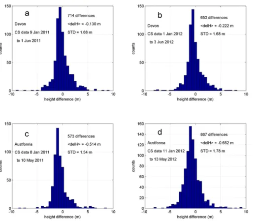
tion dataset. The airborne datasets were first referenced to the surface GPS data, and in both cases the SDs of the differences were<15 cm. The positions of the surface reference data and the centres of the CS2 footprints collected between January and May 2011 are illustrated in Fig. 3 by black and blue dots respectively. For each CS2 elevation the closest reference height was found. If the distance between the reference

20

point and the centre of the CS2 footprint was less than 400 m, the height di_fference was obtained and corrected for the slope between the two positions using the reference DEM. Although the CS2 data reflect a relatively large footprint (∼380 m along-track by

100–1500 m across-track, dependent on slopes) in comparison to the essentially point measurements from the reference data set, the mean of over 700 height differences

25

(CS2 elevation minus the reference elevation) was−0.13 m with a SD of 1.7 m (Fig. 4a).

(14)

methodol-TCD

9, 2821–2865, 2015

Arctic ice caps

L. Gray et al.

Title Page

Tables Figures

◭ ◮

Back Close

Full Screen / Esc

Discussion

P

a

per

|

Discussion

P

a

per

|

Discussion

P

a

per

|

Discussion

P

a

per

|

ogy was used to compare the ATM laser elevations against the January to May 2012 CS2 elevations. In this case the mean height difference was −0.22 m with a similar

SD (Fig. 4b). All of the CS2 data were acquired when the surface temperatures were below zero so we expect that, if calibrated correctly, the CS2 detected elevation would be lower than the actual surface elevation due to the expected volume component to

5

the CS2 returns.

Similar results were obtained in the comparison of surface and CS2 elevations for Austfonna. Again, the surface reference data were collected in the spring before any significant melt. Airborne laser (ALS) data were collected over Austfonna in spring 2011 and 2012, and surface kinematic GPS in every spring since CS2 was launched. Some

10

of the results are summarized in Fig. 4c and d. The SD of the CS2 minus surface elevation di_fferences for the two years 2011 and 2012 were comparable to the results for Devon; 1.5 m (2011) and 1.8 m (2012), but the mean height di_fferences were larger;

−0.51 m (2011) and−0.65 m (2012).

Figure 5 illustrates the individual bias points (CS2 – surface height) plotted against

15

the elevation at which they were obtained. The median elevation for each data set is marked and the mean bias for elevations above and below the median elevation are plotted with red markers. This shows that the bias between the surface and the CS2 elevation increases with elevation, particularly for Austfonna. In summary, under cold conditions any one CS2 elevation estimate will likely be lower than the surface

20

elevation, but the bias between the surface and the CS2 elevation can be dependent on the conditions of the particular ice cap.

4.2 Error estimation

The average bias between the CS2 and surface elevations changed between 2011 and 2012 for both the Devon and Austfonna data sets. Are these changes from 2011 to 2012

25

(15)

TCD

9, 2821–2865, 2015

Arctic ice caps

L. Gray et al.

Title Page

Tables Figures

◭ ◮

Back Close

Full Screen / Esc

Discussion

P

a

per

|

Discussion

P

a

per

|

Discussion

P

a

per

|

Discussion

P

a

per

|

the standard error of the mean; the SD of individual estimates divided by the square root of the number of estimates in the average. This leads to an estimate of_∼0.06– 0.07 m for the standard error of the means, implying that the year-to-year differences may be significant, and that there may have been some difference in the conditions year-to-year that led to the changing bias. However, the histograms in Fig. 4 appear

5

asymmetric so that the standard error may give an optimistic error estimate because the factors contributing to the spread in the results are not necessarily uncorrelated.

When we consider the errors in average height and height change we need to con-sider the following aspects:

1. Changes in near-surface physical characteristics: the CS2 signal will reflect from

10

the surface if it is wet (e.g. summer), but can penetrate the surface if it is cold and dry (e.g. winter). Changing historical meteorological conditions, even in winter, could change the bias between the CS2 detected surface and the true surface. We expect that the magnitude of this variable bias may be dependent on the winter accumulation and conditions.

15

2. Temporal sampling: the CS2 data acquisition occurs only on some of the 30 days in each period so that if monthly elevations are studied, some rapid changes, e.g. due to summer melt, may be underestimated. This error can be estimated for each location based on the slope of the summer height change and normally should be less than∼20 cm.

20

3. Spatial sampling – hypsometry: CryoSat-2 preferentially samples ridges and high areas since these are frequently the POCA position. Consequently, depressions and low elevation regions will be undersampled. This can be corrected when a DEM is available because we know both the ice cap hypsometry and the distri-bution of elevations used for the CS2 average height change.

25

(16)

TCD

9, 2821–2865, 2015

Arctic ice caps

L. Gray et al.

Title Page

Tables Figures

◭ ◮

Back Close

Full Screen / Esc

Discussion

P

a

per

|

Discussion

P

a

per

|

Discussion

P

a

per

|

Discussion

P

a

per

|

and the surface elevations for the different ice facies, the non-uniform sampling may lead to an additional error. These errors are di_fficult to quantify, but can be addressed on an ice-cap to ice-cap basis.

5. Altimetric corrections: there may be small systematic bias errors related to factors such as signal strength and surface slope, together with inaccuracies in

atmo-5

spheric corrections.

In general, these errors have to be addressed on an ice-cap to ice-cap basis. The sampling errors, 2 to 4, will be greatest for the 30 day height changes due to the smaller sample sizes used, and should be small for year-to-year elevation change estimates when many thousands of points are averaged. Likewise, the noise and uncertainty

10

in the CS2 results increases when analyzing separate regions due to the use of fewer points than from the ice cap as a whole. When estimating year-to-year elevation change the error associated with a possible year-to-year bias change is likely less than the combined contributions of the temporal and spatial sampling for the 30 day data set that would occur by, for example, considering end of summer height from year-to-year.

15

In summary, although the SD of CS2 estimates in relation to the surface elevation was∼1.7 m for the Devon and Austfonna in the springs of 2011 and 2012, care should

be taken in generalizing this result. The histograms (Fig. 4) appear asymmetric and the standard error of the mean may give an optimistic error estimate for an average of CS2 elevations over a specific area and time period. Of course, when considering an

20

elevation change, the bias between the surface and the CS2 elevation is unimportant as long as it has not changed in the time period between the two averages. The 0.09 and 0.14 m differences between the CS2 data and the reference data in 2011 and 2012 for Devon and Austfonna implies that this may happen, and that the possibility cannot be ignored.

(17)

TCD

9, 2821–2865, 2015

Arctic ice caps

L. Gray et al.

Title Page

Tables Figures

◭ ◮

Back Close

Full Screen / Esc

Discussion

P

a

per

|

Discussion

P

a

per

|

Discussion

P

a

per

|

Discussion

P

a

per

|

5 Ice Cap results and discussion

In this section we present CS2 elevation results, first for Devon Ice Cap, using them to illustrate the elevation changes over time, and the correlation with independent surface elevation measurements and temperature data from sensors on an automatic weather station (AWS). Comparisons are also made with airborne Ku band altimeter results.

5

The same approach is used when interpreting the height change data from the other ice caps.

5.1 Devon Ice Cap

We use_∼60 000 CS2 elevation estimates over Devon acquired from June 2010 to the end of December 2104 (Fig. 6). The separation into the NW (blue) and SE (maroon)

10

sectors allows a comparison of regions with di_fferent accumulation. Although there are clear dips in the CS2 elevations during the two warm summers in 2011 and 2012, it is apparent that some of the CS2 elevation changes don’t follow the AWS relative surface height change measurements during the cold winter-spring period (Fig. 7a and b). Indeed for the 2012–2013 winter the CS2 heights decrease from October to April

15

when, as shown by the height sensor, the surface height change should be relatively stable. While there is a slow downslope component of the AWS sensor movement, this explains just part of the discrepancy. Also, in February–March 2014 there is a dip in the CS2 derived height which is unlikely to be real.

The apparent differences between the CS2 and surface elevations suggest that

un-20

der freezing temperatures the bias between the physical surface and the derived CS2 height does change with meteorological conditions. The variation in backscattered power with position and depth of penetration recorded by the CReSIS Ku band al-timeter flown in both 2011 and 2012 shows that the waveforms vary significantly year-to-year at the same position, and in any one year with changing position (Fig. 8). In

25

(18)

TCD

9, 2821–2865, 2015

Arctic ice caps

L. Gray et al.

Title Page

Tables Figures

◭ ◮

Back Close

Full Screen / Esc

Discussion

P

a

per

|

Discussion

P

a

per

|

Discussion

P

a

per

|

Discussion

P

a

per

|

that while the airborne altimeters can see subsurface layers it is very unlikely that the CS2 altimeter could resolve these features. The reason is not just the higher resolution of the airborne systems but rather the large difference in the footprint size. In general, the shape of the leading edge of the CS2 return waveform is related to the time rate of change of illuminated area (controlled essentially by the topography), and the relative

5

surface and volume backscatter. The link between the CS2 waveform shape and the ice cap topography was demonstrated by the success in simulating CS2 waveforms using only CS2 timing and position data, and the DEM produced by swath processing the CS2 data (Gray et al., 2013).

It is difficult to deconvolve the effect of surface topography and volume backscatter

10

in traditional satellite altimetry data (Arthern et al., 2001), and the same is true for the delay-Doppler processed CS2 data. Consequently, the CS2 waveforms will be affected by the multiple layer and volume backscatter, but it is very unlikely that the CS2 could resolve the kind of layering that is visible in Fig. 8. It is possible that the changing nature of the winter accumulation reduces the surface reflectivity in relation to the

vol-15

ume component, such that the bias between the surface and the CS2 detected height increases during the winter. This could then contribute to the apparent decrease in surface height seen in the 2012/13 winter.

The only time period when we can be confident that the peak return is simply related to the surface height is during the summer period when the solar illumination and above

20

zero surface temperatures lead to snow metamorphosis, a wet surface snow layer, densification and melt. With a wet surface layer the dominant returns will be from the surface as losses increase for the component transmitted into the firn volume due to the presence of moisture.

Bearing this in mind, we can now begin to interpret the progression of CS2 derived

25

(19)

TCD

9, 2821–2865, 2015

Arctic ice caps

L. Gray et al.

Title Page

Tables Figures

◭ ◮

Back Close

Full Screen / Esc

Discussion

P

a

per

|

Discussion

P

a

per

|

Discussion

P

a

per

|

Discussion

P

a

per

|

initial CS2 height increase, there was a clear decrease in CS2 height throughout the rest of the summer, coincident in time with melting temperatures and thus interpreted as representing a real surface height decrease. This surface elevation decrease can therefore provide an estimate of summer ablation and snow/firn compaction. Following from this, accumulation can then be estimated by di_fferencing the minimum height in

5

one summer with the early summer peak the following year, although this requires extensive melt across the ice cap for both summers, so would apply only for the winter 2011–2012 accumulation on Devon Ice Cap.

There is a marked contrast between the large CS2 derived height losses during the warm summers (June–August) of 2011 and 2012, compared to 2013, when there were

10

low temperatures and little surface melt (Fig. 7c). How well the CS2 height changes represent summer melt can be assessed by comparison with the AWS and mass bal-ance pole data. From this it is clear that the maximum in accumulation and melt occur in the SE (Fig. 7a; maroon line vs. blue line). Comparing the NW CS2 height changes with those measured at the lowest AWS, which at 1317 m is the closest to the

av-15

erage height of the NW sector CS2 measurements, a good correspondence is found; 0.72±0.3 m (CS2) vs. 0.64 m (AWS) for 2011, and 0.44±0.3 m (CS2) vs. 0.67 m (AWS)

for 2012.

As described in the methods section, we can minimize the uncertainties introduced by temporal and spatial sampling by considering the ice cap wide average CS2 winter

20

elevation change (red markers in Fig. 7a). Again, we find a correspondence between the average CS2 winter elevation change with the surface elevation change recorded at the AWS at 1317 m, averaged over the same period (Fig. 7b). However, because the AWS is fixed to the upper firn layers of the ice cap, it only provides a relative measure of surface height change. The red markers (Fig. 7b) indicate the AWS height change

25

corrected for the 0.16±0.05 m a−1 vertical displacement measured by GPS between

(20)

TCD

9, 2821–2865, 2015

Arctic ice caps

L. Gray et al.

Title Page

Tables Figures

◭ ◮

Back Close

Full Screen / Esc

Discussion

P

a

per

|

Discussion

P

a

per

|

Discussion

P

a

per

|

Discussion

P

a

per

|

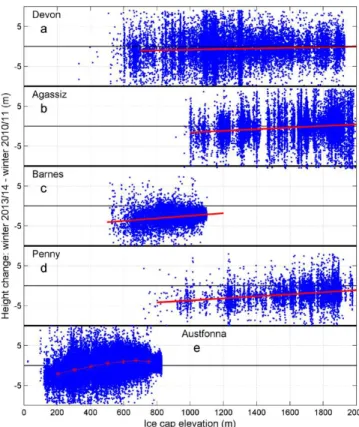
The 3 year elevation change as a function of elevation (Fig. 9a) for Devon was obtained by di_fferencing closely spaced elevation measurements from two time peri-ods; the winter of 2013/2014 minus elevations from the first winter of CS2 operation (2010/2011). This indicates that surface elevation decrease has been greatest at lower altitudes.

5

5.2 Austfonna

The CS2 data coverage of Austfonna is relatively good, due to the ice cap’s high latitude and moderately sloped surface topography: over 100 000 CS2 height estimates have been used in our analysis over the CS2 time period to the end of 2014. This allows the data set to be split into 3 sub-regions with distinct mass balance characteristics, without

10

introducing unacceptable sampling errors (Fig. 10). We define a southern (fawn) and northern (pink) region extending from the margin to 600 m elevation and a summit re-gion (green) above 600 m. Here, we exclude the area which has been strongly affected by the ongoing surge in Basin-3 (McMillan et al., 2014b; Dunse et al., 2015).

The CS2 elevation change for all three regions shows a clear drop during the summer

15

melt period (Fig. 11a), and, as expected, is smaller for the high elevation region. The largest summer height decreases were detected in 2013. This is in agreement with spring 2014 field observations indicating very strong ablation during summer 2013, and is also reflected in the air temperature recorded by the AWS station on Etonbreen (Fig. 11b).

20

As discussed for Devon, and expected from the ASIRAS results, the fluctuations in the high temporal resolution CS2 height change data suggests that under cold condi-tions there can be a variable bias between the surface and CS2 derived heights. With the larger accumulation and milder, more variable winter temperatures on Austfonna one would expect the variable bias problem to be more severe than on Devon. For

25

(21)

TCD

9, 2821–2865, 2015

Arctic ice caps

L. Gray et al.

Title Page

Tables Figures

◭ ◮

Back Close

Full Screen / Esc

Discussion

P

a

per

|

Discussion

P

a

per

|

Discussion

P

a

per

|

Discussion

P

a

per

|

in April of around−15◦C, before warm air moves in at the beginning of May

accompa-nied by a significant snow fall. The apparent CS2 height increase of_∼1–1.5 m over the southern coastal areas is therefore likely explained by a shift from volume to surface scatter and a real height change associated with fresh, probably wet, snow.

In the northern and summit region there is an overall increase in average

eleva-5

tion over the CS2 time frame (Figs. 11a and 12). The total winter-to-winter eleva-tion increase for the summit region is ∼1 m over the three years from 2010/2011 to

2013/2014. This took place primarily in the first two years and there was little change in average high altitude elevation between the winters of 2012/2013 and 2013/2014, spanning the large melt in the summer of 2013 (Fig. 11a). The northern side shows

10

a winter-to-winter increase in elevation for the first two years, which then dips to an overall increase in 3 years of∼0.5 m. This dip may also be related to the large 2013

melt. In contrast, the southern region has lost elevation. This may be explained partly by the hypsometry of Bråsvellbreen (Basin 1 in Fig. 12), a surge type glacier in its qui-escent phase since the last surge in 1936/1937. A large fraction of the glacier lies at

15

low elevations, and is characterized by strong ablation.

We derived the height change over 3 years by taking all the height data from the last year of data acquisition, November 2013 to December 2014, and subtracting the heights from July 2010 to December 2011 (Fig. 12). Individual pairs of height estimates within 400 m were di_fferenced, slope corrected and binned into footprints of _∼1 km2.

20

The most striking feature is the large height decrease of>_{30 m associated with the} surge of Basin-3. Otherwise, the pattern of interior thickening, especially along the east side of the main ice divide, and the marginal thinning resembles the elevation-change pattern reported for earlier time periods (Bamber et al., 2004; Moholdt et al., 2010). Also, the CS2 height change results are consistent with the results obtained from

re-25

(22)

TCD

9, 2821–2865, 2015

Arctic ice caps

L. Gray et al.

Title Page

Tables Figures

◭ ◮

Back Close

Full Screen / Esc

Discussion

P

a

per

|

Discussion

P

a

per

|

Discussion

P

a

per

|

Discussion

P

a

per

|

The 3 year height loss as a function of elevation for all the Austfonna data, but with the Basin 3 data removed, mirrors the situation in Canadian Arctic ice caps (Fig. 9e). The height loss decreases with increasing elevation although the linear approximation used for the others isn’t appropriate in this case.

5.3 Barnes Ice Cap

5

On Barnes Ice Cap the relative maximum power of each return waveform shows in-creased power and dynamic range in the summers (Fig. 13a), which we interpret to be a consequence of the presence of moisture in the snow, melt and the possibility of a specular return from a wet surface. The 30 day CS2 height changes (Fig. 13b) clearly show significant ice loss due to the warm summers in 2011 and 2012, with much lower

10

losses in 2013 and 2014 due to the colder summers in those years.

Each year there is a small height increase in June, immediately prior to the height loss due to summer melt (Fig. 13b). This is consistent with the observations for Devon and Austfonna, and is interpreted as the transition from a composite surface and vol-ume signal to one dominated by the snow surface as melt begins. The height loss due

15

to summer melt each year ranged from 1.38 to 2.55 m, whereas winter accumulation, estimated from the summer minimum in one year to the maximum at the onset of melt in the following year, remained relatively constant at∼1 m each winter. It is therefore

clear from the high temporal resolution data that summer melt is dominant in defining the annual mass balance. Estimating errors is more straightforward for Barnes because

20

of the simpler configuration of surface facies: the ice cap consists essentially of snow over ice in winter, with the loss of all the winter snow the following summer. In this case we base the error estimate on the statistics of the 50+estimates of each height change: the error bars on the elevation change estimates (Fig. 13b) indicate±2 times

the standard error of the mean. This approach has not been used for the other ice caps

25

(23)

TCD

9, 2821–2865, 2015

Arctic ice caps

L. Gray et al.

Title Page

Tables Figures

◭ ◮

Back Close

Full Screen / Esc

Discussion

P

a

per

|

Discussion

P

a

per

|

Discussion

P

a

per

|

Discussion

P

a

per

|

error in summer height loss due to melt associated with the temporal sampling is also smaller than for Devon.

When analyzing the winter-to-winter height change results derived from the average of the December to May data each year (red dots in Fig. 13b), it is evident that between winter 2010/2011 and winter 2013/2014 Barnes Ice Cap lost 2.73±0.30 m in average

5

elevation, with most of that loss occurring in the summers of 2011 and 2012. These numbers agree well with the high temporal resolution height change estimates. An increase in melt at lower elevations on the ice cap is also observed (Fig. 9c), an effect originally shown by the work of Abdalati et al. (2004) and confirmed in the work of Gardner et al. (2012).

10

5.4 Agassiz and Penny Ice Caps

At 81◦N the Agassiz Ice Cap receives less accumulation and has much less summer melt than the Penny Ice Cap on southern Ba_ffin Island (67◦_{N). The magnitudes of the} peak CS2 returns reflect these different surface temperature regimes: Agassiz expe-rienced relatively less melt than Penny at high elevations even in the warm 2011 and

15

2012 summers, consequently the seasonal variation in the peak returns is much less (Fig. 14a and b). The e_ffect of summer melt on the CS2 returns is obvious in the Penny results (Fig. 14c and d). The strong peak returns even at high elevations at the end of July imply a strong specular reflection from a wet ice surface.

The increased time gap between the groups of passes evident for Penny in

compari-20

son to those from Agassiz is due to the fact that the ascending and descending passes over Penny occurred in the same time period, as well as the influence of the spreading of the passes due to the lower latitude.

There is little point in attempting to assess at the monthly height change for ei-ther ice cap as ei-there is simply not enough data (Table 1). However, winter-to-winter

25

(24)

TCD

9, 2821–2865, 2015

Arctic ice caps

L. Gray et al.

Title Page

Tables Figures

◭ ◮

Back Close

Full Screen / Esc

Discussion

P

a

per

|

Discussion

P

a

per

|

Discussion

P

a

per

|

Discussion

P

a

per

|

2011/2012, 2012/2013 and 2013/2014 with respect to the winter of 2010/2011 show a larger ice loss for Penny in relation to Agassiz (Fig. 14e). Again the e_ffect of the warm 2011 and 2012 summers, and the contrast with the summer of 2013, is evident. On both ice caps, height loss decreases with increasing elevation (Fig. 9b and d).

The di_fferent climate regime between Agassiz and Penny is obvious in the contrast

5

between the plots of the peak returns in Fig. 14 (a, b vs. c, d). This implies that the bias between surface and CS2 detected surface will be less variable for Agassiz than Penny, and that the errors in surface height change will be smaller. This is reflected in the estimates of potential errors in the year-to-year height change (Table 1).

6 Conclusions

10

The airborne Ku band altimeter results over Devon and Austfonna imply that there will be a variable bias between the physical surface and the heights derived from CryoSat-2. This has been confirmed with our analysis of CS2 data; with ice cap wide melt the bias between the CS2 height and the physical surface will be a minimum in the summer, but will increase with winter accumulation and the change in the nature of

15

the surface. The transition from freezing temperatures to melt in the early summer is accompanied by an increase in the CS2 elevation, but without an equivalent increase in the surface height. This corresponds to the transition from a composite surface-volume backscatter to one dominated by the surface. Under freezing conditions the bias between the CS2 derived elevation and the physical surface appears to vary with

20

the current and historical conditions on the ice cap in a way that is hard to quantify although for Austfonna the difference appears to increase with increasing elevation.

Notwithstanding the uncertainty in the bias between the surface and CS2 elevation, the winter-to-winter CS2 height change results can give a credible estimate of ice cap surface height change. The largest uncertainty in these estimates, and the most difficult

25

(25)

TCD

9, 2821–2865, 2015

Arctic ice caps

L. Gray et al.

Title Page

Tables Figures

◭ ◮

Back Close

Full Screen / Esc

Discussion

P

a

per

|

Discussion

P

a

per

|

Discussion

P

a

per

|

Discussion

P

a

per

|

in near surface density would also affect the density one should use in estimating the mass change based on the volume change. However, the results for the Canadian ice caps show clearly the large year-to-year height decrease associated with the strong summer melt in 2011 and 2012. All show a net height loss over the CS2 time period, although Devon and Agassiz show a modest height increase after the low summer

5

2013 melt. This is in contrast to Austfonna where the summer of 2013 showed the largest melt induced height loss although the upper elevations of the ice cap appears to be still gaining elevation since mid-2010 when CryoSat-2 was commissioned. However, all the ice caps show a height loss at their lower elevations.

For the first time, CryoSat-2 has provided credible monthly height change results

10

for some relatively small ice caps, and the summer surface height decrease has been identified and measured. For some of the ice caps this allows the estimation of both accumulation and summer melt. For Barnes, thanks to the absence of firn, the CS2 results provide an excellent record of change since the fall of 2010. The continued loss of elevation even after the relatively cold snowy summer of 2013 attests to the eventual

15

demise of this ice cap. The key CS2 attribute which has made these advances possible is the ability to geocode the footprint position.

Acknowledgements. This work was supported by the European Space Agency through the provision of CryoSat-2 data and the support for the CryoVex airborne field campaigns in both the Canadian Arctic and Svalbard. NASA supported the IceBridge flights over the Canadian

20

Arctic, while NSIDC and the University of Kansas (CreSIS) facilitated provision of the airborne laser and radar altimetry data. The Technical University of Denmark (TUD) managed the ESA supported flights over Devon and Austfonna. The IceBridge and TUD teams are gratefully ac-knowledged for the acquisition of the airborne data used in this work. The Polar Continental Shelf Project (Natural Resources Canada) provided logistic support for field work in the

Cana-25

dian Arctic, and the Nunavut Research Institute and the communities of Grise Fjord and Res-olute Bay gave permission to conduct research on the Agassiz and Devon ice caps. Support for D. Burgess and M. N. Demuth was provided through the Climate Change Geoscience Pro-gram (Contribution # 20150076), Earth Sciences Sector, Natural Resources Canada and the GRIP programme of the Canadian Space Agency. Support for K. Langley was provided by ESA

(26)

TCD

9, 2821–2865, 2015

Arctic ice caps

L. Gray et al.

Title Page

Tables Figures

◭ ◮

Back Close

Full Screen / Esc

Discussion

P

a

per

|

Discussion

P

a

per

|

Discussion

P

a

per

|

Discussion

P

a

per

|

project Glaciers-CCI (4000109873/14/I-NB). Wesley Van Wychen and Tyler de Jong helped with the 2011 kinematic GPS survey on Devon. NSERC funding to L. Copland is also gratefully acknowledged.

References

Abdalati, W., Krabill, F., Manizade, S., Martin, C., Sonntag, J., Swift, R., Thomas, R., Yungel, J.,

5

and Koerner, R.: Elevation changes of ice caps in the Canadian Arctic Archipelago, J. Geo-phys. Res.-Earth, 109, F04007, doi:10.1029/2003JF000045, 2004.

Abdalati, W., Zwally, H. J., Bindschadler, R., Csatho, B., Farrell, S. L., Fricker, H. A., Harding, D., Kwok, R., Lefsky, M., Markus, T., Marshak, A., Neumann, T., Palm, S., Schutz, B., Smith, B., Spinhirne, J., and Webb, C.: The ICESat-2 laser altimetry mission, Proc. IEEE, 98, 735–751,

10

2010.

Andrews, J. T. and Barnett, D. M.: Holocene (Neoglacial) moraine and proglacial lake chronol-ogy, Barnes Ice Cap, Canada, Boreas, 6, 341–358, 1979.

Arthern, R. J., Wingham, D. J., and Ridout, A. L.: Controls on ERS altimeter measurements over ice sheets: footprint-scale topography, backscatter fluctuations, and the dependence of

15

microwave penetration on satellite orientation, J. Geophys. Res.-Atmos., 106, 33471–33484, doi:10.1029/2001JD000498, 2001.

Baird, P. D.: Method of nourishment of the Barnes ice cap, J. Glaciol., 2, 2–9, 1952.

Bamber, J., Krabill, W., Raper, V., and Dowdeswell, J.: Anomalous recent growth of part of a large Arctic ice cap: Austfonna, Svalbard, Geophys. Res. Lett., 31, L12402,

20

doi:10.1029/2004GL019667, 2004.

Bell, C., Mair, D., Burgess, D., Sharp, M., Demuth, M., Cawkwell, F., Bingham, R., and Wad-ham, J.: Spatial and temporal variability in the snowpack of a high Arctic ice cap: implications for mass-change measurements, Ann. Glaciol., 48, 159–170, 2008.

Bouzinac, C.: CryoSat-2 Product Handbook, Tech. Report, European Space Agency,

avail-25

able at: https://earth.esa.int/documents/10174/125272/CryoSat_Product_Handbook, last access: 26 February 2014.

(27)

TCD

9, 2821–2865, 2015

Arctic ice caps

L. Gray et al.

Title Page

Tables Figures

◭ ◮

Back Close

Full Screen / Esc

Discussion

P

a

per

|

Discussion

P

a

per

|

Discussion

P

a

per

|

Discussion

P

a

per

|

measurements on the ice cap Austfonna, Svalbard, The Cryosphere Discuss., 2, 777–810, doi:10.5194/tcd-2-777-2008, 2008.

Burgess, D. O.: Mass balance of the Devon (NW), Meighen, and South Melville ice caps, Queen Elizabeth Islands for the 2012–2013 balance year, Open File 7692, Geological Survey of Canada, Ottawa, Canada, p. 26, doi:10.4095/295443, 2014.

5

Burgess, D. O., Sharp, M. J., Mair, D. W. F., Dowdeswell, J. A., and Benham, T. J.: Flow dynam-ics and iceberg calving rates of the Devon Island ice cap, Nunavut, Canada, J. Glaciol., 51, 219–238, doi:10.3189/172756505781829430, 2005.

Davis, C. H.: A robust threshold re-tracking algorithm for measuring ice-sheet surface el-evation change from satellite radar altimeters, IEEE T. Geosci. Remote, 35, 974–979,

10

doi:10.1109/36.602540, 1997.

Davis, C. H. and Segura, D. M.: An algorithm for time-series analysis of ice sheet surface elevations from satellite altimetry, IEEE T. Geosci. Remote, 39, 202–206, 2001.

de la Peña, S., Nienow, P., Shepherd, A., Helm, V., Mair, D., Hanna, E., Huybrechts, P., Guo, Q., Cullen, R., and Wingham, D.: Spatially extensive estimates of annual accumulation in the dry

15

snow zone of the Greenland Ice Sheet determined from radar altimetry, The Cryosphere, 4, 467–474, doi:10.5194/tc-4-467-2010, 2010.

Dowdeswell, J. A.: Drainage-basin characteristics of Nordaustlandet ice caps, Svalbard, J. Glaciol., 32, 31–38, 1986.

Dowdeswell, J. A., Drewry, D., Cooper, A., Gorman, M., Liestøl, O., and Orheim, O.: Digital

map-20

ping of the Nordaustlandet ice caps from airborne geophysical investigations, Ann. Glaciol., 8, 51–58, 1986.

Dowdeswell, J. A., Benham, T. J., Strozzi, T., and Hagen, J. O.: Iceberg calving flux and mass balance of the Austfonna ice cap on Nordaustlandet, Svalbard, J. Geophys. Res., 113, F03022, doi:10.1029/2007JF000905, 2008.

25

Dunse, T., Schuler, T. V., Hagen, J. O., Eiken, T., Brandt, O., and Høgda, K. A.: Recent fluctua-tions in the extent of the firn area of Austfonna, Svalbard, inferred from GPR, Ann. Glaciol., 50, 155–162, 2009.

Dunse, T., Schellenberger, T., Hagen, J. O., Kääb, A., Schuler, T. V., and Reijmer, C. H.: Glacier-surge mechanisms promoted by a hydro-thermodynamic feedback to summer melt, The

30