ISSN 1546-9239
© 2008 Science Publications
Corresponding Author: Mohammad Naisipour, Department of Civil Engineering, University of Science and Technology, Tehran, Iran,
Collocation Discrete Least Squares (CDLS) Method for Elasticity Problems and Grid
Irregularity Effect Assessment
1
M. Naisipour,
1M. H. Afshar,
2B. Hassani,
1A. R. Firoozjaee
1
Department of Civil Engineering, University of Science and Technology, Tehran, Iran
2
Department of Civil Engineering, University of Technology, Shahrood, Iran
Abstract: A meshless approach, collocation discrete least square (CDLS) method, is extended in this paper, for solving elasticity problems and grid irregularity effect is assessed. In the present CDLS method, the problem domain is discretized by distributed field nodes. The field nodes are used to construct the trial functions. The moving least-squares interpolant is employed to construct the trial functions. Some collocation points that can be independent of the field nodes are used to form the total residuals of the problem. The least-squares technique is used to obtain the solution of the problem by minimizing the summation of the residuals for the collocation points. The final stiffness matrix is symmetric and therefore can be solved directly via efficient solvers. The boundary conditions are easily enforced by the penalty method. The present method does not require any mesh so it is a truly meshless method. Numerical examples are studied in detail, which show that the present method is stable and possesses good accuracy, high convergence rate and high efficiency for both regular and irregular point distribution.
Keywords: Meshless method, MLS, Least square technique, CDLS, Elasticity, Irregular grids INTRODUCTION
The finite element method (FEM) has been the most frequently used numerical method in engineering during the three past decades. It has been used in most fields of applied sciences such as computational solid mechanics [1, 2, and 3] and so on. Mesh-based methods are not well suited to the problems associated with extremely large deformation and problems associated with frequently remeshing. To avoid these drawbacks of the FEM, a new class of numerical methods, meshless methods (also called mesh-free methods) have been developing [4, 5] in the recent decade. These methods have become an important tool in computational solid mechanics, owing to their advantages over the traditional finite element method (FEM), volume method (FVM), and finite-difference method (FDM). Meshless methods rely only on a group of scatter points, which means not only that the burdensome work of mesh generation is avoided, but also more accurate description of irregular complex geometries can be achieved. Furthermore, the meshless approximation has higher smoothness, and no additional post-processing is needed.
In the field of meshless methods for solving elasticity problems, Krysl and Belytschko [6] employed
Element-Free Galerkin Method (EFGM) to analyze thin plates; Onate et al. [7] proposed a stabilization technique by introducing new terms in both the governing equations and the traction boundary conditions to solve elasticity problems; Kwon et al. [8] presented a least-squares meshfree method for solving linear elastic problems; Zhang et al. [9] proposed a meshless weighted least-squares (MWLS) method, to solve problems of elastostatics; Atluri et al. proposed a MLPG mixed collocation method [10] and MLPG mixed finite difference method [11] for solid mechanics.
establishment of the weak form demands accurate integration [14]. In addition, because meshless shape functions are too complex to be expressed in closed form, a delicate background mesh and a large number of quadrature points are always employed, which decreases the efficiency seriously. As a consequence, GBMMs are much more computationally expensive than the FEM [15].
The other group of meshless methods is built on collocation schemes. The SPH, FPM, least-square collocation meshless method [16], and point weighted least-square (PWLS) method [17] all belong to this group. These methods are very efficient and easy to program, but they usually suffer from poor stability, and the accuracy often goes down near the boundary.
The universal law of least squares can be used for discretization. In fact, it has been introduced into the FEM successfully [18]. A truly meshless method based on the least-squares approach, the collocation discrete least-squares (CDLS) method, was proposed to solve Poisson’s equation [19] and free surface seepage problem
[20]
and also was presented for error estimation and adaptive refinement in one dimensional fluid mechanics
[21]
. Because of using the least-squares technique and more collocation points the CDLS method is not bothered by instability as collocation-based meshless methods. In this research the CDLS method is extended for elasticity problems and effect of grid irregularity is assessed.
MATERIALS AND METHODS
In the present CDLS method, the problem domain is discretized by distributed field nodes. The field nodes are used to construct the trial functions by employing the moving least-squares interpolant. Some collocation points that can be independent of the field nodes are used to form the total residuals of the problem. The least-squares technique is used to obtain the solution of the problem by minimizing the summation of the residuals for the collocation points.
Moving least square shape functions: Among the available meshless approximation schemes, the moving least squares (MLS) method [22] is generally considered to be one of the best methods to interpolate random data with a reasonable accuracy, because of its completeness, robustness and continuity [10, 23]. With the MLS interpolation, the unknown function is approximated by:
T
where PT (X) is a polynomial basis in the space coordinates, and m is the total number of the terms in the basis. For a 2D problem we can specify T
for . is the vector of
coefficients and can be obtained by minimizing a weighted discrete L2norm as follows:
T
The weight function is usually built in such a way that it takes a unit value in the vicinity of the point j where the function and its derivatives are to be computed and vanishes outside a region Ω surrounding the point and N is the number of nodes in the domain. In this research the cubic spline weight function is considered as follows:
d
where ⁄ and is the size of influence domain of point .
Minimization of equation (2) leads to where
w
, , … ,
Comparing equation (4) with the well known form of equation (7) yields to equation (8)
T
T T
where T contains the shape functions of nodes at point which are called moving least square (MLS) shape functions.
Collocation discrete least square (CDLS) method: Consider the following partial differential equation
Ω
Subject to appropriate Dirichlet and Neumann boundaries
where L and B are partial differential operators and f
represents external forces or source term on the problem domain.
partial differential equation at a typical collocation point k is:
, ~
The residual of Neumann boundary condition at typical collocation k on the Neumann boundary can also be written as:
, ~
and finally the residual of Dirichlet boundary condition at collocations on the Dirichlet boundary could be stated by:
, ~
where Mt is the number of collocation points on the
Neumann boundary, Mu is the number of collocation
points on the Dirichlet boundary and M is the total number of collocation points. A penalty approach is used to form the total residual of the problem defined as:
where and are penalty coefficients for Neumann and Dirichlet boundary conditions respectively.
Minimization of the functional with respect to nodal parameters , , , . . . , leads to the following system of equations:
where
T
T
T
T
T
T
The stiffness matrix K in Eq. (16) is square , symmetric and positive definite. Therefore,
the final system of equations can be solved directly via efficient solvers.
RESULTS AND DISCUSSION
In this section, two 2D numerical examples, which are solved by the CDLS method, are presented. The examples include: 1) a cantilever beam under end point load, and 2) an infinite plate with a circular hole under uniaxial load which is solved with both regular and irregular node distribution.
Fig. 1: A cantilever beam under a point load at the end
Fig. 2: The nodal configuration of the cantilever beam for d=0.5 (125 nodes, 221 collocation points)
Cantilever beam: A cantilever beam under a point load at the end (see Fig. 1) is solved as the first example. For this problem, the exact stress and displacement solution for plane stress is given in Timoshenko and Goodier [24] as
0
And
where / is the moment of inertia for a beam with rectangular cross-section and unit thickness. The problem is solved using the CDLS method under plane stress condition with the following constants: ,
E = 1000, c = 1, L =12 and v = 0.3.
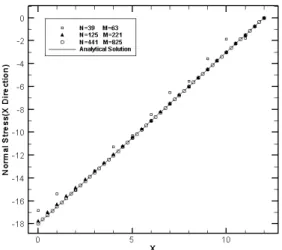
collocation points are 63, 221, and 825, respectively. The nodal configuration for d = 0.5 is shown in Fig. 2. This problem is simulated using the MLS with the second order polynomial basis. Fig. 3 shows the vertical displacement along the central line of the beam for the three nodal configurations. The simulation results agree with the analytical solution very well. Fig. 4 shows the stress at stations along upper surface of the cantilever beam for the three nodal configurations and a very good agreement with the analytical solution is obtained. The contours of stress displayed over the deformed shape for the nodal configuration with d = 0.25 are shown in Fig. 5.
Fig. 3: The vertical displacement of the cantilever beam under the end load
Fig. 4: Stress at stations along upper surface of the cantilever beam
The convergence rate is studied with three nodal configurations (d =1.0, 0.5, and 0.25). The following error norm is used for showing the convergence rate in Fig. 6:
∑ ∑
where N is the total number of nodes, and are the approximation and exact stress values at node , respectively.
The results clearly show that a stable convergence rate is obtained for the present CDLS method.
Fig. 5: Contours of stress displayed over the deformed shape(Regular grid of 441 nodes)
Fig. 6: The convergence rate in the cantilever beam under the end load
Fig. 7: An infinite plate with a circular hole under a uniaxial load
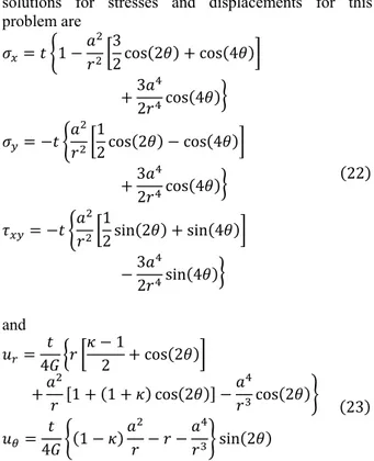
solutions for stresses and displacements for this problem are
cos cos
cos
cos cos
cos
sin sin
sin
and
cos
cos cos
sin
respectively. In the above equations, G is the shear modulus and ⁄ with v the Poisson’s ratio. Due to symmetry, only the upper right square quadrant of the plate is modeled [see Fig. 8]. The edge length of the square is 5a, with a being the radius of the circular hole. The exact analytical displacements solution is imposed on the left and bottom edges, and
the tractions obtained from the analytical solution [Eq. 22] are applied to the top and right edges. The periphery of the circular hole is traction-free.
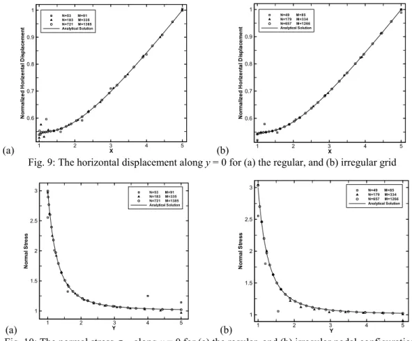
The problem is solved using the CDLS method, under a plane stress condition, with the following constants: t =1, E = 1000, and v=0.3. For assessment of grid irregularity effect on results of CDLS method, three regular nodal configurations with 53, 183 and 721 nodes, respectively, and also three irregular nodal distributions with 49, 179 and 657 nodes, respectively, are used. The regular and irregular grids with 183 and 179 nodes, respectively, are shown in Fig. 8. The MLS with quadratic basis is used in the simulation. The horizontal displacement along the bottom edge (y = 0), and the stress component along the left edge (x
= 0) obtained with the regular and irregular grids are shown in Fig. 9 and Fig. 10, respectively. The contours of stress obtained with the regular and irregular nodal configurations of 721 and 657 nodes are plotted in Fig. 11. Compared with the analytical solutions, good agreements are obtained for both the displacements and stresses. These results also show that the CDLS method possesses good accuracy for both regular and irregular grids.
Fig. 12 shows convergence rate with three regular nodal configurations (n =53, 183, and 721) and three irregular nodal configurations (n =49, 179, and 657). A stable and monotonic convergence rate is observed for the problem. It is remarkable that similar convergence rates are obtained for both regular and irregular grids.
(a) (b)
Fig. 8: Infinite plate with a circular hole. (a) The regular grid (N=183, M=335), and (b) the irregular grid (N=179,
(a) (b)
Fig. 9: The horizontal displacement along y = 0 for (a) the regular, and (b) irregular grid
(a) (b)
Fig. 10: The normal stress along x = 0 for (a) the regular, and (b) irregular nodal configurations
(a) (b)
Fig. 11: The normal stress σ contours displayed over the deformed shape. (a) Regular grid of 721 nodes, and (b) irregular grid of 657 nodes
CONCLUSION
In this article, the collocation discrete least square (CDLS) method is extended to solve elasticity problems and grid irregularity effect is assessed. The final coefficient matrix obtained by the present method is
symmetric and therefore can be solved directly via efficient solvers. The boundary conditions are easily enforced by penalty method. Because of no need to any mesh, this method is a truly meshless method. Results of the numerical examples show that the present method is stable and have good accuracy, high
X N o rm al iz ed H o ri z en tal D is p lac em en t
1 2 3 4 5
0.6 0.7 0.8 0.9 1 N=53 M=91 N=183 M=335 N=721 M=1385 Analytical Solution X N o rm a liz e d H o ri z e n ta l D isp la ce m e n t
1 2 3 4 5
0.6 0.7 0.8 0.9 1 N=49 M=85 N=179 M=334 N=657 M=1266 Analytical Solution Y N o rm a l S tre s s
1 2 3 4 5
1 1.5 2 2.5
3 N=53 M=91
N=183 M=335 N=721 M=1385 Analytical Solution Y N o rm a l S tre s s
1 2 3 4 5
1 1.5 2 2.5
3 N=49 M=85
convergence rate and high efficiency for both regular and irregular grids. All of these advantages of the CDLS ensure that it is a very potential meshless method for the applications in elasticity problems.
Fig. 12:The convergence rate of the infinite plate with a circular hole
REFERENCES
1. Labibzadeh, M. and S.A. Sadrnejad, 2006. Mesoscopic damage based model for plane concrete under static and dynamic loadings. American Journal of Applied Sciences, 3 (9): 2011-2019.
2. Labibzadeh, M. and S.A. Sadrnejad, 2007. Crack analysis of concrete arch dams using micro-planes damage based constitutive relations. American Journal of Applied Sciences, 4 (4): 197-202.
3. Labibzadeh, M., S.A. Sadrnejad and M. Naisipour, 2008.An Assessment of Compressive Size Effect of Plane Concrete Using Combination of Micro-Plane Damage Based Model and 3D Finite Elements Approach. American Journal of Applied Sciences, 5 (2): 106-109.
4. Belytschko, T., Y. Krongauz, D. Organ, M. Fleming, and P. Krysl, 1996. Meshless methods: an overview and recent developments. Comput. Meth. Appl. Mech. Eng., 139: 3–47.
5. Liu G. R., 2002. Mesh free methods: moving beyond the finite element method. CRC press, USA.
6. Belytschko T, P. Krysl, 1995. Analysis of thin plates by the element-free Galerkin method. Computational Mechanics. 17: 26-35.
7. Onate E., F. Perazzo, J. Miquel, 2001, A finite point method for elasticity problems, Computers and Structures, 79: 2151-2163.
8. Kwon, K. C., S. H. Park, B. N. Jiang, and S. K. Youn, 2003, The least-squares meshfree method for solving linear elastic problems, Computational Mechanics, 30: 196-211.
9. Zhang, X., X. F. Pan, W. Hu, and M. W. Lu, 2002, Meshless weighted least-square method, Fifth World Congress on Computational Mechanics, Vienna, Austria.
10. Atluri, S. N., H. T. Liu, Z. D. Han, 2006, Meshless Local Petrov-Galerkin (MLPG) mixed collocation method for elasticity problems, CMES: Computer Modeling in Engineering & Sciences, 14: 141-152. 11. Atluri, S. N., H. T. Liu, Z. D. Han, 2006, Meshless Local Petrov-Galerkin (MLPG) mixed finite difference method for solid mechanics, CMES: Computer Modeling in Engineering & Sciences, 15: 1-16.
12. Belytschko, T., Y. Lu, and L. Gu, 1994, Element Free Galerkin Method, Int. J. Numer. Meth. Eng, 37: 229–256.
13. Beissel, S., and T. Belytschko, 1996, Nodal integration of the element-free Galerkin method, Comput. Meth. Appl. Mech. Eng, 139: 49–74. 14. Park, S. H., and S. K. Youn, 2001, The least-square
meshfree method, Int. J. Numer. Meth. Eng, 52: 997–1012.
15. Pan, X., K. Y. Sze, X. Zhang, 2004, An assessment of the meshless weighted least-square method, Acta Mechanica Solida Sinica, 17: 270-282.
16. Zhang, X., X. H. Liu, K. Z. Song, and M. W. Lu, 2001, Least-square collocation meshless method, Int. J. Number. Meth. Eng, 51: 1089–1100.
17. Wang, Q. X., H. Li, K. Y. Lam, 2005, Development of a new meshless – point weighted least–squares (PWLS) method for computational mechanics, Computational Mechanics, 35: 170– 181.
18. Jiang, B. N., 1998, the least-squares finite element method: theory and applications in computational fluid dynamics and electromagnetics, chap. 1, Springer-Verlag, Berlin.
19. Arzani1, H., and M. H. Afshar, 2006, Solving Poisson’s equations by the discrete least square meshless method, WIT Transactions on Modeling and Simulation, 42: 23–31.
20. Firoozjaee, A. R., and M. H. Afshar, 2007, Collocation discrete least square meshless method for the solution of free surface seepage problem, International Journal of Civil Engineering, 5(2): 134-143
21. Afshar, M. H, and M. Lashckarbolok, 2007, Collocated discrete least square (CDLS) meshless method: error estimate and adaptive refinement, Int. J. Numer. Meth. Fluids, in press.
22. Lancaster, P., and K. Salkauskas, 1981, Surfaces generated by moving least squares method. Mathematics of computation, 37: 141-158.
23. Atluri, S. N., 2004, The Meshless Local Petrov-Galerkin (MLPG) method for domain & boundary discretizations, Tech Science Press.
24. Timoshenko, S. P., and J. N. Goodier, 1987, Theory of elasticity, 3rd edition, McGraw-Hill, New York.
ln(sqrt(N))
ln
(E
rr
o
r
No
rm
)
1 1.2 1.4
-2 -1.5 -1 -0.5