UNIVERSIDADE DA BEIRA INTERIOR
Engenharia
Analysis of Slender Aircraft Structures using the
Finite Element Method
Filipe José Robalo Fraqueiro
Dissertação para obtenção do Grau de Mestre em
Engenharia Aeronáutica
(Ciclo de estudos integrado)
Orientador: Prof. Pedro Vieira Gamboa
Acknowledgement
I want to thank my parents for supporting me during these last years and for never having doubts about my capabilities. I also want to thank Professor Pedro Vieira Gamboa for having supervising me during this work and for the knowledge that he passed to me. And thank to my other professors during this course. Finally I want to thank my friends and a special thanks to Pedro Albuquerque that helped me to improve some important soft skills.
Resumo
Actualmente há uma grande exigência para que as análises estruturais sejam o mais realistas possiveis e altamente fiáveis. Na indústria aeronáutica isto é traduzido numa redução de peso das aeronaves mantendo os factores de segurança desejados. Porém este tipo de análises são um processo demorado e trabalhoso e por vezes é necessário apresentar uma solução mais rápida, embora menos fiável, que possa ser utilizada como ponto de partida no projecto preliminar. Existem diversos métodos para resolver os diferentes problemas estruturais. Quando os casos são simples é possivel chegar a uma solução analítica, porém estes casos são muito reduzidos e envolvem a resolução de equações diferenciais. Assim é necessário recorrer a métodos numéri-cos de interpolação ou de aproximação. Um destes métodos é o método dos elementos finitos. Este método consiste em dividir o domínio do problema em pequenas fracções, chamadas de elementos, e aplicar aproximações em cada uma dessas fracções tendo em consideração os re-sultados das fracções envolventes. No caso desta dissertação este método é aplicado do ponto de vista unidimensional (1D), ou seja, as estruturas são do tipo: viga, barra de tracçao e barra de torção e os elementos são representados por segmentos de recta. Os pontos inicias e fi-nais destes segmentos são chamados de nós e permitem a continuidade da estrutura estando conectados aos elementos adjacentes.
Duas grandes tarefas foram executadas neste trabalho. Inicialmente o método matemático dos elementos finitos foi ajustado para uma análise estrutural, mais concretamente em estruturas que possam ser consideradas em uma dimensão, e para determinar a deformação da estrutura sob determinados carregamentos e condições de fronteira. É ainda possivel calcular os modos de vibração livre da estrutura. Depois este método foi aplicado num algoritmo de forma a poder ser programado e aplicado a diversos casos.
De modo a verificar a fiabilidade do código desenvolvido foram estudados alguns casos com diferentes dados iniciais. Estes dados iniciais referem-se: ao tamanho e perfil da estrutura, material, cargas aplicadas e condições de fronteira, sendo os resultados comparados com pro-gramas já existentes no mercado, verificando assim se são plausíveis.
Palavras-chave
Análise Estrutural, Método dos Elementos Finitos, Viga, Condições de Fronteira, Equações Difer-enciais
Abstract
At present there is a great demand for structural analysis to be as realistic as possible and highly reliable. In the aeronautical industry this is translated into a reduction of the aircrafts weight and maintaining the desired safety factors. However, this type of analysis is a time-consuming and labor-intensive process and sometimes it is necessary to have a faster, but less reliable, solution that can be used as a starting point in the preliminary design.
There are several methods for solving the different structural problems. When the cases are simple it is possible to have an analytical solution, however these cases are reduced and in-volves the resolution of differential equations. Thus it is necessary to use numerical methods of interpolation or approximation. One of these methods is the finite element method. This method consists in dividing the problem domain into small fractions, called elements, and apply-ing approximations in each of these fractions takapply-ing into account the results of the surroundapply-ing fractions. In the case of this dissertation this method is applied from a one-dimensional (1D) point of view, ie, the structures are of the type: beam, bar and rod and the elements are rep-resented by straight line segments. The start and end points of these segments are called nodes and allow the continuity of the structure and they are connected to the adjacent elements. Two major tasks were performed in this work. Initially the mathematical method of the fi-nite elements was adjusted for a structural analysis, more concretely in structures that can be considered in one dimension, and to determine the deformation of the structure under certain loads and boundary conditions. It is still possible to calculate the free vibration modes of the structure. Then this method was applied to an algorithm so that it could be programmed and applied to several cases.
In order to verify the reliability of the developed code some cases with different initial data were studied. These initial data refers to: the size and cross-section of the structure, material, loads and boundary conditions. The results are compared with programs that already exist in the market, thus verifying if they are plausible.
Keywords
Contents
1 Introduction 1
1.1 Motivation . . . 1
1.2 Objectives . . . 2
1.3 Thesis Outline . . . 2
2 The Finite Element Method 5 2.1 Historical Overview . . . 5 2.2 Constitutive model . . . 8 2.3 Bar Problem . . . 10 2.4 Rod Problem . . . 16 2.5 Beam 1 Problem . . . 21 2.6 Beam 2 Problem . . . 29 2.7 General Problem . . . 33 3 Code Development 39 3.1 Code Structure . . . 39
3.2 Inputs and Outputs . . . 42
3.3 Cross-Section . . . 44
4 Code Validation 47 4.1 Selection of Analysis Cases . . . 47
4.2 Results Comparison . . . 47
4.2.1 Case 1 . . . 48
4.2.2 Case 2 . . . 49
4.2.3 Case 3 . . . 51
4.2.4 Case 4 . . . 52
6 Conclusion 63
6.1 Conclusions . . . 63
6.2 Future Work . . . 63
List of Figures
2.1 Differential Equations Analysis Methods. . . 6
2.2 Historical Evolution of the FEM [OCZ00]. . . 6
2.3 Algorithm for a FEM Analysis [Bat14]. . . 7
2.4 Bar Loads . . . 10 2.5 Bar Displacements . . . 12 2.6 Bar Matrices . . . 17 2.7 Rod Loads . . . 17 2.8 Rod Displacements . . . 19 2.9 Beam 1 Loads . . . 21 2.10 Beam 1 Displacements . . . 23 2.11 Beam 2 . . . 30 2.12 Beam 2 Displacements . . . 31 2.13 Rotation Angles. . . 36 2.14 Matrices Assembly. . . 37
3.1 Code Flow Chart. . . 40
3.2 Mesh Generation. . . 41
3.3 Code Main Program. . . 41
3.4 Code Variables. . . 41
3.5 General data inputs. . . 42
3.6 Structure data inputs. . . 42
3.7 BC and loads inputs. . . 43
3.8 Cross-section and material database inputs. . . 43
3.9 Instant Results Windows. . . 43
3.10 Tecplot Results. . . 44
3.12 Skin Section. . . 44
3.13 C shaped Section. . . 45
4.1 Circular cross-section. . . 48
4.2 C-channel cross-section. . . 49
4.3 Ansys Free Vibration Modes. . . 50
4.4 Code Free Vibration Modes. . . 50
4.5 Square Tube cross-section. . . 51
4.6 Ansys Circular Section Mesh. . . 52
4.7 Code Circular Section Mesh. . . 52
4.8 Case 4 Results. . . 53
5.1 NACA0012 Skin represented by CATIA V5. . . 56
5.2 NACA0012 Skin represented by Code. . . 56
5.3 Ansys Analysis Steps. . . 57
5.4 Code Analysis Cross-Sections. . . 57
5.5 Code Analysis Cross-Sections Properties. . . 57
5.6 SOLID186 Element. . . 58
5.7 SURF154 Element. . . 58
5.8 Comparison of Bending for Blade 1. . . 59
5.9 Comparison of Bending for Blade 2. . . 59
5.10 Comparison of Bending for Blade 3. . . 60
5.11 Comparison of Bending for Blade 4. . . 60
5.12 Comparison of Bending for Blade 5. . . 61
List of Tables
4.1 Material Properties. . . 47
4.2 Case 1 results comparison. . . 48
4.3 Case 2 results comparison. . . 49
4.4 Case 3 results comparison. . . 51
5.1 Blades Definition. . . 55
5.2 Cross-section properties comparison using code and CATIA V5. . . 55
5.3 Volume and Mass comparison using code and CATIA V5. . . 56
List of Acronyms
BC Boundary Conditions
CAD Computer Aided Design
DE Differential Equation
DOF Degrees of Freedom
EO Equation of Motion
FDM Finite Differences Method
FEA Finite Element Analysis
FEM Finite Element Method
ID Identification Number
IE Integral Equation
PVW Principle of Virtual Work
1D One Dimension
List of Symbols
A Cross section area
C Constitutive matrix
cu Compressive strength
D Differentiation matrix
d Approximation displacements vector
E Young’s modulus e Element EA Axial stiffness EI Bending stiffness F Loads matrix G Shear modulus GJ Torsional stiffness
Ip Inertial polar moment
Iψ Warping moment
i x-axis unit vector
J Torsional Constant
j y-axis unit vector
k z-axis unit vector
K Rigidity matrix
l Length
m Mass
Mx Concentrated torsion momentum
My Concentrated bending momentum
Mz Concentrated bending momentum
N Number of elements
N Approximation Local coordinates vector
Px Concentrated normal force
Py Concentrated shear force
Pz Concentrated shear force
Qx Distributed normal force
Qy Distributed shear force
Qz Distributed shear force
rote Element rotation matrix
s Displacements vector
t Time
tu Tensile strength
u Linear displacement along x direction
v Linear displacement along y direction
w Linear displacement along z direction
Wext External Work
Wextinertia External inertia Work
Wint Internal Work
Wx Distributed torsion momentum
Wy Distributed bending momentum
Wz Distributed bending momentum
X Space coordinates vector
x x-axis coordinate
y y-axis coordinate
List of Greek Symbols
γ Shear strain
ε Normal strain
ε Strain matrix
bε Strain vector
θx Angular displacement along x direction
θy Angular displacement along y direction
θz Angular displacement along z direction
ν Eigenvector ν Poisson’s ratio ξ Local variable ρ Density σ Normal Stress σ Stress matrix bσ Stress vector τ Shear stress
ϕhe Horizontal rotation angle
ϕve Vertical rotation angle
ϕxe x-axis rotation angle
ψ Warping function
Chapter 1
Introduction
1.1
Motivation
One of the most important objectives in aircraft design and other engineering activities is to achieve the most reliable product with the lowest possible costs. So, it is very important to per-form accurate calculations using the minimum computational resources possible. In structural analysis, this accurate calculation can result in a weight reduction and in aerospace engineering this means that the aircraft can be more efficient and have lower manufacturing and operational costs. The use of less resources is also important to preserve the planet environment.
In the present day there are some computer software packages that perform finite element analysis (FEA) such as ANSYS [ANS18], Dassault Systèmes ABAQUS [Das18] and MSPATRAN [MSC18]. These software packages have years, or even decades, of development and perform multiple types of analyses. However, to legally use those commercially available software packages a paid license is required. Another disadvantage is that the user must have some knowledge and experience to use these software because they have a large number of available models and tools.
Considering this disadvantages it would be very useful a simple and user friendly tool, that allows a simple and fast structural analysis to calculate structures displacements. This tool aims to be used in structures that could be assumed with just one dimension (1D) and allow all the six space degrees of freedom (DOF).
Analysing propellers and wing spars to check if them resist and deform to flight loads are some applications that motivate the development of the present work. This applications should also have analysing-time benefits because this tool should perform quick analysis. Other motivation for the development of a structural analysis code is that it could be incorporated in an optimiza-tion problem. For example, in propeller structural analysis there is the possibility of coupling this code to an aerodynamics analysis code where the loads that result from this last code can be applied in the structural one and the result is a new shaped propeller that can be again subjected to the aerodynamics code. This are commonly known as aerostructural analysis. As a low-fidelity method it prove to be superior over their high-fidelity counterparts when a high number of model evaluations are required as for instance when performing a design optimization since high-fidelity analyses are often very time-consuming, like [JS14] explained.
There are several applications of the finite element method (FEM) using 1D elements in civil, naval and aeronautical structures. In naval structures [EC16] uses 1D beam models claiming that those are much simpler compared to three dimensions (3D) solid FEM. Also, [EC13] uses 1D models, for the same reason presented before, when the objective is to analyse slender bodies, such as columns, rotor-blades, aircraft wings, towers and bridges. The both use 1D
elements formulated with Euler–Bernoulli and Timoshenko beam models to determine structures deformations and free vibration modes. Although one limitation with the Euler–Bernoulli beam models is that they ignore the transverse shear stresses or, in a best option, it is assumed as constant over the beam cross-section. The 1D element theories do not capture cross-section warping.
1.2
Objectives
The main objective of this thesis is to develop a simple and user-friendly tool to perform FEA in one dimension so that a preliminary study of the stiffness characteristics of a beam-like slender structure can be performed in an efficient and accurate way. This FEA is applied to structural engineering and in this case, it calculates the six displacements in a cartesian reference frame: three axial displacements and three angular displacements. It also aims to allow the computa-tion of the structure free vibracomputa-tion modes. The meaning of 1D analysis is that the code should be able to recognise structures of beam type, in order words, one of the structure dimensions is relatively larger than the other two. This tool consists in a Fortran [Wik18] code that reads the required inputs from a text file. It also needs to be tested in order to satisfy the mechanical requirements of the propellers analysed in [Mor16] and guarantee its reliability.
Furthermore, a validation of the tool should be performed, through the comparison with a mature software that have years of development like Ansys.
1.3
Thesis Outline
To accomplish the objectives, the first task is to study the mathematical model of the finite element method for the problem described. After studying this model, it is possible to check the required analysis variables that produce the desired results. Then it is fundamental to apply a coherent algorithm that translates the results of the mathematical model. After these two steps, some simple cases are selected to verify if the results are plausible and compare them with other available software solutions. Finally, a case study can be performed to complete the code validation.
Chapter 2 features a brief history of finite element analysis background. This chapter allows the understanding of the power of this method and provides a brief theoretical explanation of how it is applied in this context. It also explains the mathematical model that supports the method. The results of this model are the code algorithm and inputs. It also provides a bridge between the structures physical properties and its deformations when subjected to certain loads. Chapter 3 describes the computational code and the details about the cross-section properties, that are important to study beam type structures.
Chapter 4 presents the work done to validate the code. To validate the code some structures are selected and then are applied to the developed code, those structures are also analysed in ANSYS software. Then both results are compared, calculating the deviation between both,
after that the differences and similarities are discussed.
Chapter 5, similarly to chapter 4, describes a case study to validate the code. In this case study the code inputs are five blades, designed in [Mor16], with different geometries, materials and loads. The results from those analysis are compared with the ones obtained in CATIA V5 software by [Mor16] and Ansys.
Chapter 6 presents the general discussion and conclusions of the work developed during the current dissertation and some possible future works to achieve better results.
Chapter 2
The Finite Element Method
This chapter show the maths that formulates the finite element method. As explained in the previous chapter, this method can be used in various fields of physics, maths and engineering. So it is necessary adapt the method to this thesis case: displacements of 1D structures. In order to do that it is first necessary to establish the relations between this displacements and the extensions and tensions that the structure can experience. Then, three different 1D structures are considered: rod, bar and beam, the last one is also divided in two. This is required to study the different displacements, once each one has different behaviours for the different loads directions. The 1D elements for the different types are formed by two tip nodes and the displacements variations along the elements is linear.
2.1
Historical Overview
Before developing a practical tool, it is fundamental to understand the theoretical principle of the finite element method and its origins. A brief historical description of the development of this analysis methodology is present in this chapter.
In physics and engineering there are a lot of problems that are mathematically expressed using differential equations (DE) and integral equations (IE). Problems such as fluid flows, heat trans-fer, mass transtrans-fer, vibrations of structures, electromagnetic interactions and stress and strain of structures [Bat14] are represented by complex equations and require different methods to be solved. Some simple equations have an exact solution and are solvable by explicit formulas. However, most DE, and the ones presented in this dissertation, require numerical methods to be solved. Figure 2.1 resumes some methods to solve analytic and numeric DE.
One of the first methodologies to solve DE was the finite differences method (FDM). This repre-sents a group of numerical methods to solve the DE that uses approximations in the derivatives of the differential equations. Other techniques like various weighted residual procedures or approximate techniques for determining the stationary of a properly defined functional were also developed by mathematicians, as Figure 2.2 shows. All these discretization methods use approximations to represent a continuum solution but, they were not intuitively enough for some problems. So, engineers found a more intuitive way to solve them by creating an analogy between real discrete elements and finite portions of a continuum domain [OCZ00]. This was called finite element method.
A vast number of engineers, physicists and mathematicians had contributed for the development and evolution of this methodology. According to [Bat14], the original contributions appeared in the papers by J. H. Argyris and S. Kelsey; M. J. Turner, R. W. Clough, H. C. Martin, and L. J. Topp, and R. W. Clough in 1950s. The first and perhaps the simplest definition of the
Figure 2.1: Differential Equations Analysis Methods.
Figure 2.2: Historical Evolution of the FEM [OCZ00].
finite element process states that: “the continuum is divided into a finite number of parts (elements), the behaviour of which is specified by a finite number of parameters, and the solution of the complete system as an assembly of its elements follows precisely the same rules as those applicable to standard discrete problems”.
This methodology was being developed side by side with the digital computer and they comple-ment each other. This means that to achieve better results with FEM the number of elecomple-ments should be studied and refined and the use of computers reduces the calculation time. Otherwise
the most precise analysis would take so much time that it would be impractical to solve cer-tain problems. One of the first companies that developed software which used finite element analysis (FEA) was ANSYS in 1970.
To perform a FEA it is required to follow a methodology, summarized in Figure 2.3, before achieving the final solution. First, it is necessary to look at the physical problem and define the mathematical differential equations to solve, including the boundary and initial conditions. Then, the domain needs to be split to define the elements and its nodes and create the so-called mesh. After doing this, it is possible to solve the DE using FEM, although it is then necessary to look at the results and check if they are plausible. If not, the mathematical model needs to be verified to check if some physical incoherence is present or if the mesh is incorrectly defined. If the outputs are physically plausible, a mesh refinement can be done to achieve better accuracy. This last step needs to be performed considering the hardware properties, because with a very detailed mathematical model or with many elements and nodes (or both) a large amount of computer memory and processor capacity is required.
Figure 2.3: Algorithm for a FEM Analysis [Bat14].
In the present days FEA is strongly related with computer aided design (CAD) and because of that one other step can be added to this methodology that is the graphical representation of the results. This helps the user to check if the process was done correctly because he has a clear image of the entire process.
2.2
Constitutive model
In structural mechanics the constitutive model is no more than an equation that establishes the relation between stresses and strains. The strains are linear and angular displacements in a deformable body [Meg07]. They are the quotient between the deformation suffered and the initial length of a small element within the structure. So, it is first required to define a vector 2.1 that represent the spacial displacement that can occur.
s(x, y, z, t) = u(x, y, z, t) v(x, y, z, t) w(x, y, z, t) (2.1)
This vector is filled with the displacements u, v and w in the three space directions x, y and z respectively. These displacements are time dependent, once they can vary in time depending on the loads applied. However, the work developed in this thesis ignores the time dependence of the displacements. In other words, this is a static analysis where just the space variables are required 2.2. X = x y z (2.2)
It is also necessary to define a unit vector that is associated with the orientation of each axis and those are defined by the letters i, j and k for the x-, y- and z-axis respectively. It is then possible to calculate the strains 2.3 along each axis and in the different planes.
εij = 1 2 ( ∂si ∂Xj + ∂sj ∂Xi ) (2.3)
As it is possible to check in 2.4 in the main diagonal of the matrix there are represented the strains along each axis normal strain detonated by ε (sub axis) and the strains in the planes -shear strain - detonated by γ (sub plane). This is a symmetric matrix therefore it is equivalent to the final column matrix of 2.5.
ε = εxx γxy γxz γyx εyy γyz γzx γzy εzz = ∂u ∂x 1 2( ∂u ∂y + ∂v ∂x) 1 2( ∂u ∂z + ∂w ∂x) 1 2( ∂v ∂x+ ∂u ∂y) ∂v ∂y 1 2( ∂v ∂z + ∂w ∂y) 1 2( ∂w ∂x + ∂u ∂z) 1 2( ∂w ∂y + ∂v ∂z) ∂w ∂z (2.4)
bε = εxx εyy εzz 2γxy 2γxz 2γyz (2.5)
So, to have coherence in the constitutive model, the constitutive matrix 2.6 is a six by six matrix. Its content is provided by studying the material and its properties, so it is entirely dependent of the material that is being analysed and strongly affects the final results of the structural analysis. C = C11 C12 C13 C14 C15 C16 C21 C22 C23 C24 C25 C26 C31 C32 C33 C34 C35 C36 C41 C42 C43 C44 C45 C46 C51 C52 C53 C54 C55 C56 C61 C62 C63 C64 C65 C66 (2.6)
Finally, it is possible to determine the stress vector using Hooke’s law 2.8. This law states
that the Cauchy stressbσ tensor 2.9 is the result of the product of stiffness tensor (constitutive
matrix) and strain tensor (assumed as strain vector for simplicity purposes). The normal stress is detonated by σ (sub axis) and the shear stress by τ (sub plane).
σ = σxx τxy τxz τyx σyy τyz τzx τzy σzz (2.7) bσ = Cbε (2.8) bσ = σxx σyy σzz τxy τxz τyz (2.9)
matrix 2.10. In this matrix the three first diagonal terms are the Young’s modulus (E) and are related with the normal strains and the other three are shear modulus (G) that are related with the shear strains. The relationship between those two constants is given by Equation 2.11 using the Poisson’s ratio (ν).
C = E 0 0 0 0 0 0 E 0 0 0 0 0 0 E 0 0 0 0 0 0 G 0 0 0 0 0 0 G 0 0 0 0 0 0 G (2.10) G = E 2(1 + ν) (2.11)
As already enunciated above, the structure is studied taking into account three different sub problems that are divided accordingly the loads and displacements orientation. This three prob-lems are described in the following chapter’s sub-sections.
2.3
Bar Problem
The first case is the bar element which withstands only axial loads, represented in Figure 2.4, and undergoes only axial displacements. Those loads can be concentrated on any of the two
extremities of the bar element, Px, or may be distributed along its length, Qx.
Figure 2.4: Bar Loads
The first step is to reduce the space displacements vector just to the axial displacement along x-axis 2.12. Then the strain 2.13 and stress 2.14 vectors are obtained from equations 2.5 and 2.9 respectively.
ε = εxx= εx= ∂u ∂x (2.13) σ = σxx= σx= C11εx= E ∂u ∂x (2.14)
The next step is to determine the dynamic equilibrium equations. There are several ways to achieve this:
1. Newton’s second law; 2. D’Alembert’s principle; 3. Energetic formulation;
4. Principle of virtual work (PVW); 5. General dynamics equation; 6. Lagrange equation.
For this thesis the principle chosen was the principle of virtual work because it easily enables to introduce the virtual variations that will be hereafter replaced by the approximation functions.
So, the variation of the internal work δWint is determined by Equation 2.15 and it is equal to
the variation on the stress within the body volume dV .
δWint=
∫
V
δεxσxdV (2.15)
Replacing θx and σx by 2.13 and 2.14 the variation of internal work is now represented by
Equation 2.16. δWint= ∫ V δ∂u ∂xE ∂u ∂xdV (2.16)
This volume integral is then decomposed in an area integral where the cross-section properties of the structure are present and a length variation that gives us the 1D shape for the FEM. It is assumed that the material properties do not change across the cross-section area, so it is possible to assume EA as the rod axial stiffness and obtain 2.17.
δWint= ∫ l δ∂u ∂xEA ∂u ∂xdx (2.17)
On the other side of the principle of virtual work is the variation of the external work δWext. The
variation work of inertia forces δWextinertiaand the variation work of the applied loads δWextloads
are here represented 2.18.
δWext= δWextinertia+ δWextloads (2.18)
Analysing the loads applied to the bar element (Figure 2.4) the variation of the external work is determined using Equation 2.19. The inertia load is the product of the displacement s and the bar density ρ. δWext=− ∫ V δsρ¨sdV + ∫ l δsQxdx + δu(0, t)Px0+ δu(l, t)Pxl (2.19)
In Equation 2.19 the general displacement vector s can be replaced by the respective displace-ment for this case as Equation 2.12 shows. And once again, the volume integral is decomposed to obtain a length integral where it is possible to apply the FEM. It is also assumed that the material properties do not change across the section’s area it is possible to assume m as the rod’s mass per unit of length (= ρ A). The final Equation 2.20 for the variation of the external work is then obtained.
δWext=− ∫ l δum¨udx + ∫ l
δuQxdx + δu(0, t)Px0+ δu(l, t)Pxl (2.20)
The next required step is to obtain the approximation functions for the displacement that will be applied in the PVW. Let us assume the discretization of the position domain looking for a single element with two nodes 2.5.
Figure 2.5: Bar Displacements
Let us introduce some variables that are illustrated in the Figure 2.5:
ξ- position along the element
uj(t) - displacement of the element right node
le- length of the element
uj−1is at ξ = 0 and uj is at ξ = 1
Now it is required to have the relation between ξ and x 2.21 because the FEM approximation considers a local displacement instead of global one. So, ξ is the local space variable for each element and it is dependent on the global position and the element length. It is also necessary to have the relation between this new local variable and the variation of the global position x of the element 2.22.
ξ = x− (j − 1)le
le
(2.21)
dx = ledξ (2.22)
After understanding this changing of variables, a linear interpolation is applied to interpolate the element’s displacement between the two nodes 2.23.
u(ξ, t) = a + bξ (2.23)
And with the boundary conditions 2.24 it is possible to determine the constants a 2.25.
u(0, t) = u1 u(1, t) = u2 (2.24) a = u1 b = u2− u1 (2.25)
The final approximation function for de displacement u 2.26 is obtain by replacing the constants
aand b in 2.23 with 2.25.
u(ξ, t) = (1− ξ)u2+ ξuj (2.26)
Equation 2.26 can be written in a vector form 2.27 assuming a vector for the nodes displacement 2.28 and one for the local position variable 2.29.
u(ξ, t) = N (ξ)de(t) (2.27) de(t) = [ u1(t) u2(t) ] (2.28) N (ξ) = [ 1− ξ ξ ] (2.29) dN dξ = [ −1 1] (2.30)
And lastly, analysing the PVW equations, the variation of this approximation function 2.31 it is also required.
δu(ξ, t) = N (ξ)δdej(t) (2.31)
Going back to the PVW the internal and external work must be equal 2.32 and 2.33.
δWint= δWext (2.32) ∫ l δ∂u ∂xEA ∂u ∂xdx =− ∫ l δum¨udx + ∫ l
δuQxdx + δu(0, t)Px0+ δu(l, t)Pxl (2.33)
Since vectors and matrices in Equation 2.33 require some algebraic multiplication it is necessary to transpose the first displacement in each equation’s term. This will lead to Equation 2.34.
∫ l δ∂u ∂x T EA∂u ∂x =− ∫ l δuTm¨udx + ∫ l
δuTQxdx + δuT(0, t)Px0+ δuT(l, t)Pxl (2.34)
Finally, it is possible to perform the coordinate change 2.35 and insert the approximation func-tion and starting by consider just one element the final FEM equafunc-tion for this problem is achieved 2.37.
∫ 1 0 δ∂(N de) T ∂ξle EAe ∂(N de) ∂ξle ledξ = − ∫ 1 0 (N δde)TmeN ¨deledξ + ∫ 1 0 (N δde)TQxeledξ + (N (0)δde) TP x1+ (N (1)δde)TPx2 (2.35) δdTe 1 le ∫ 1 0 ∂NT ∂ξ EAe ∂N ∂ξ dξde= −δdT ele ∫ 1 0 NTmeN dξ ¨de+ δ(de)Tle ∫ 1 0 NTQxedξ + δd T eN (0)TPx1+ δdTeN (1)TPx2 (2.36) δdTeKede=−δdTeMed¨e+ δdTeFe (2.37)
In these final equations Kerepresents the stiffness matrix 2.38, Merepresents the mass matrix
2.39, Ferepresents the load vector 2.40 and dethe displacements vector 2.44 for one element.
Ke= 1 le ∫ 1 0 ∂NT ∂ξ EAe ∂N ∂ξ dξ (2.38) Me= le ∫ 1 0 NTmeN dξ (2.39) Fe= le ∫ 1 0 NTQxedξ + N T(0)P x1+ NT(1)Px2 (2.40)
Replacing in this last three equations the vector N and its variation by the Equations 2.29 and 2.30 the final matrices for the elements are:
Ke= EAe le [ 1 −1 −1 1 ] (2.41) Me leme 6 [ 2 1 1 2 ] (2.42)
Fe= leQxe 2 [ 1 1 ] + Px1 [ 1 0 ] + Px2 [ 0 1 ] (2.43) de= [ u1 u2 ] (2.44)
Up to this point it was considered just one element, although the finite element method is the assembly of several elements so it is required to perform the sum of the PVW of each element 2.45, where N is the number of elements and now the properties and loads are functions of the local coordinate ξ. N ∑ j=1 ∫ jle (j−1)le δ∂u T ∂x EAej(ξ) ∂u ∂xdx = − N ∑ j=1 ∫ jle (j−1)le δuTmej(ξ)¨udx + N ∑ j=1 ∫ jle (j−1)le δuTQxej(ξ)dx + δu T(0, t)P x1+ δuT(l, t)Px2 (2.45)
A summation of Equation 2.37 is required for all elements that leads to Equation 2.46 in which
Kej, Mej, Fej, dej are the stiffness and mass matrices and loads and displacements vector,
respectively, of element j. N ∑ j=1 δdTejKejdej=− N ∑ j=1 δdTejMejd¨ej+ N ∑ j=1 δdTejFej (2.46)
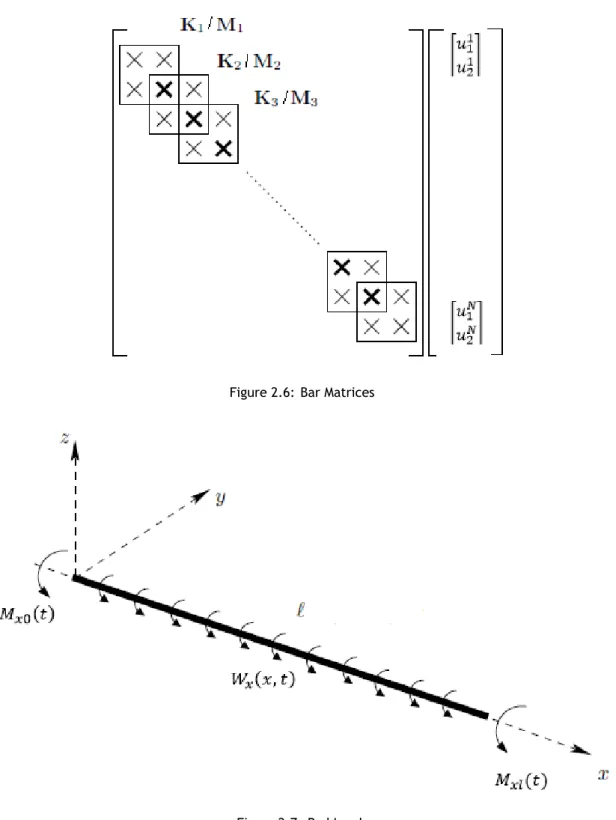
In a practical computational application, a final matrix is assembled as shown in Figure 2.6 where the result is an n vs. n matrix for the stiffness and mass matrices and a n column vector for the loads and displacements vectors, where n is the number of degrees of freedom (DOF) of the problem. For 1D linear elements the number of nodes is equal to two times the number of elements plus one.
2.4
Rod Problem
The formulation of the finite element method for a rod is similar to the bar, therefore the different steps are here demonstrated.
In Figure 2.7 it is possible to see the loads present in the rod formulation. This loads are a
distributed torsion moment Wx and two concentrated torsion moments Mx one at each rod’s
Figure 2.6: Bar Matrices
Figure 2.7: Rod Loads
The displacement in this case is the torsion along the x axis θx and the displacements vector
is now represented as shown in Equation 2.47. The ψ function is the contribution of the cross-section warping. s(x, y, z, t) = ψ(y, z)∂θx ∂x −zθx yθx (2.47)
The strain and stress vectors are obtained by substituting the displacement in Equation 2.3. ε = 0 0 0 (∂ψ∂y − z)∂θx ∂x (∂ψ∂z + y)∂θx ∂x 0 (2.48) σ = 0 0 0 G(∂ψ∂y − z)∂θx ∂x G(∂ψ∂z + y)∂θx ∂x 0 (2.49)
The variation of the internal work δWint is given by equation 2.50 and replacing ε and θ by the
values in Equations 2.48 and 2.49 it is possible to obtain Equation 2.51.
δWint= ∫ V δεσdV (2.50) δWint= ∫ V δ (( ∂ψ ∂y − z ) ∂θx ∂x ) G ( ∂ψ ∂y − z ) ∂θx ∂x + δ (( ∂ψ ∂z + y ) ∂θx ∂x ) G ( ∂ψ ∂z + y ) ∂θx ∂x dV (2.51)
The volume integral is then separated into two other integrals for the area and length and assuming that the material properties do not change across the cross-section area it is possible to assume GJ as the bar torsional stiffness and the variation of the internal work is now:
δWint= ∫ l δ∂θx ∂xGJ ∂θx ∂xdx (2.52)
Once again the variation of the external work δWextis the sum of the inertia and loads works
as represented in the following equation:
δWext= δWextinertia+ δWextloads (2.53)
δWext=− ∫ V δsρ¨sdV + ∫ l δsWxdx + δθx(0, t)Mx0+ δθx(l, t)Mxl (2.54)
Replacing in Equation 2.54 the displacement by 2.47 and after performing some algebra calcula-tions the variation of the external work for this case is given by Equation 2.55. In this equation
Iprepresents the inertial polar moment. Other constant Iψrelated to the warping of the
cross-section was derived in this step, but it was neglected because its dimension is very small when compared with the polar moment of inertia.
δWext=− ∫ l δθxIpθ¨xdx + ∫ l δθxWxdx + δθx(0, t)Mx0+ δθx(l, t)Mxl (2.55)
Then it is required to obtain the approximation function for the displacement θx. This step is
the same as the bar.
Figure 2.8: Rod Displacements
ξ- position along the element
θxj−1(t) - displacement of the element left node
θxj(t) - displacement of the element right node
le- length of the element
θxj−1 is at ξ = 0 and θxj is at ξ = 1
So the final equations are the following:
de(t) = [ θx1(t) θx2(t) ] (2.56) N (ξ) = [ 1− ξ ξ ] (2.57)
dN
dξ =
[
−1 1] (2.58)
δθx(ξ, t) = N (ξ)δdej(t) (2.59)
Going back to the PVW and replacing in Equation 2.63 by the values on the Equations 2.52 and 2.55 and transposing the matrices to allow the algebraic computations the Equation 2.61 is obtained. δWint= δWext (2.60) ∫ l δ∂θx ∂x T GJ∂θx ∂x =− ∫ l δθxTIpθ¨xdx + ∫ l δθTxWxdx + δθxT(0, t)Mx0+ δθTx(l, t)Mxl (2.61)
After performing the coordinate change to the local coordinate ξ and applying the approximation function 2.59 in the motion equation 2.61 it is possible to have the FEM equation for the rod
2.62, where it is assumed that GJ and Ipdo not change along the element.
δdTe 1 le ∫ 1 0 ∂NT ∂ξ GJe ∂N ∂ξ dξde= −δdT ele ∫ 1 0 NTIpeN dξ ¨de+ δ(de) Tl e ∫ 1 0 NTWxedξ + δd T eN (0) TM x1+ δdTeN (1) TM x2 (2.62)
The last equation 2.62 can be simplified to Equation 2.63.
δdTeKede=−δdTeMed¨e+ δdTeFe (2.63)
In which Ke, Me, Feand derepresent the stiffness 2.64 and mass 2.65 matrices and loads 2.66
and displacements 2.67 vectors respectively.
Ke= GJe le [ 1 −1 −1 1 ] (2.64)
Me= leIpe 6 [ 2 1 1 2 ] (2.65) Fe= leWxe 2 [ 1 1 ] + Mx1 [ 1 0 ] + Mx2 [ 0 1 ] (2.66) de= [ θx1 θx2 ] (2.67)
2.5
Beam 1 Problem
The general formulation of the beam problem is equal to the previous ones, the only main difference is that in this problem there are two displacements to take into account. This two
displacements are a linear displacement w and a rotation θx.
By looking to Figure 2.9 the present loads in this case are:
1. distributed load aligned with z-axis Qz;
2. distributed bending moment Wy;
3. concentrated loads aligned with z-axis Pz, one at each beam tip;
4. concentrated bending moment My, one at each beam tip.
Figure 2.9: Beam 1 Loads
To simplify this case it is possible to assume a decoupled Euler-Bernoulli beam theory so the displacements vector is represented by equation 2.68.
s(x, t) = −z∂w ∂x 0 0 (2.68)
θy =
∂w
∂x (2.69)
Assuming the relation of the previous equation 2.69 and using Equation 2.3 it is possible to achieve the strain vector 2.70 for the beam.
ε = −z∂2w ∂x2 0 0 (2.70)
Once having the strain vector, using the constitutive relation the stress vector is equal to 2.71.
σ = E −z∂2w ∂x2 0 0 (2.71)
After this first step, the second one is to calculate motion equation for the beam. To perform
this step the PVW is used and the variation of the internal work δWintis given by the following
equation:
δWint=
∫
V
δεσdV (2.72)
Using the Equations 2.70 and 2.71 in Equation 2.72, Equation 2.73 is obtained.
δWint= ∫ V δ∂ 2w ∂x2z 2E∂ 2w ∂x2dV (2.73)
In the last equation the volume integral is transformed into an area and a length integrals and assuming that the material properties do not change across the cross-section area it is possible
to assume EIyy as the beam bending stiffness. After integrate the equation by parts twice and
assuming EIyy constant along x-axis the variation of the internal work for this beam is given by
Equation 2.74. δWint= [ δ∂w ∂xEIyy ∂2w ∂x2 ]l 0 − [ δwEIyy ∂3w ∂x3 ]l 0 + ∫ l δwEIyy ∂4w ∂x4dx (2.74)
work done by the beam inertia and the external loads applied as Figure 2.9 shows. The inertial loads are related with the displacement s and the beam density ρ.
δWext= δWextinertia+ δWextloads (2.75)
The Equation 2.75 is then rewritten as Equation 2.76.
δWext=− ∫ V δsρ¨sdV + ∫ l δwQzdx ∫ l δ∂w ∂xWydx + δw(0, t)Pz0+ δw(l, t)Pzl+ δ∂w ∂x(0, t)My0+ δ ∂w ∂x(l, t)Myl (2.76)
Once again it is assumed that the material properties do not change across the cross-section area and remember the Equation 2.69 the variation of the external work is:
δWext=− ∫ l δwm ¨wdx + ∫ l δwQzdx + ∫ l δθyWydx + δw(0, t)Pz0+ δw(l, t)Pzl+ δθy(0, t)My0+ δθy(l, t)Myl (2.77)
Then it is necessary to have the approximation function for the displacements. Like the previous cases lets start by assuming a variable change. It is assumed the discretization of the position domain looking for a single element with two nodes, as represented in 2.10.
Figure 2.10: Beam 1 Displacements And it is also required to assume some variables:
ξ- position along the element
wj−1(t) - displacement of the element left node
wj(t) - displacement of the element right node
θyj(t) - displacement of the element right node
le- length of the element
wj−1is at ξ = 0 and wj is at ξ = 1
θyj−1 is at ξ = 0 and θyj is at ξ = 1
The first step is to calculate the relation between ξ and x, that is given by Equation 2.78 and the variation by 2.79.
ξ = x− (j − 1)le
le
(2.78)
dx = ledξ (2.79)
Similar to the bar and rod cases a linear interpolation is used in order to interpolate the el-ement displacel-ement between the two nodes. Although, for the beam problem there are four displacements to take into account, so a fourth order polynomial function is used 2.80.
w(ξ, t) = a + bξ + cξ2+ dξ3 (2.80)
And using the boundary conditions w(0, t) and w(1, t) it is possible to have the relations 2.81 and 2.82.
w1= a (2.81)
w2= a + b + c + d (2.82)
And perform the derivative of equation 2.80:
dw
dξ = b + 2cξ + 3dξ
2
(2.83)
Remember the relation between the vertical displacement w and the θyfor the first node, where
dw
dx(0) = θy1 (2.84)
And using the equation 2.79 it is possible to have the derivative of the displacement w in function of the local coordinate ξ 2.85.
dw
dξ(0) = le
dw
dx(0) (2.85)
After combining Equations 2.84 and 2.85, Equation 2.86 is reached:
dw
dξ(0) = leθy1 (2.86)
And finally applying Equation 2.83 for the first node where the local coordinate is zero it is possible to have the relation 2.87.
leθy1 = b (2.87)
Using the same explanation as above for the second node it is possible to have the relation 2.88.
leθy1 = b + 2c + 3d (2.88)
It is now possible to combine the Equations: 2.81, 2.82 2.87 and 2.88 to have an equation system 2.89. w1= a leθy1= b w2= a + b + c + d leθy2= b + 2c + 3d (2.89)
a = w1 b = leθy1 c = w2− w1− leθy1− d 3d = leθy2− leθy1− 2(w2− w1− leθy1− d) (2.90) a = w1 b = leθy1 c = w2− w1− leθy1− d d = leθy2− leθy1− 2w2+ 2w1+ 2leθy1 (2.91) a = w1 b = leθy1 c =−3w1− 2leθy1+ 3w2− leθy2 d = 2w1+ leθy1− 2w2+ leθy2 (2.92)
After solving the equation system it is possible to have the constants 2.92 of the approximation equation 2.80 and rewrite it as Equation 2.93.
w(ξ, t) = w1(1− 3ξ2+ 2ξ3) + leθy1(ξ− 2ξ
2+ ξ3) + w
2(3ξ2− 2ξ3) + leθy2(−ξ
2+ ξ3)
(2.93)
The last equation can be compacted in a matrix form where N is the local coordinate matrix
2.96 and dethe displacement matrix 2.95 for the two nodes of the element.
w(ξ, t) = N (ξ)de(t) (2.94) de(t) = w1(t) θy1(t) w2(t) θy2(t) (2.95) N (ξ) = [ 1− 3ξ2+ 2ξ3 l e(ξ− 2ξ2+ ξ3) 3ξ2− 2ξ3 le(−ξ2+ ξ3) ] (2.96)
Analysing the equations of the internal 2.74 and external 2.77 work it is required to have the first and second derivatives of the displacement function w in function of ξ. So these derivatives are represented in Equations 2.97 and 2.98.
dN dξ = [ −6ξ + 6ξ2 l e(1− 4ξ + 3ξ2) 6ξ− 6ξ2 le(−2ξ + 3ξ2) ] (2.97) d2N dξ2 = [ −6 + 12ξ le(−4 + 6ξ) 6 − 12ξ le(−2 + 6ξ) ] (2.98)
It is also necessary to have the variation of w:
δw(ξ, t) = N (ξ)δdej(t) (2.99)
Matching the equation of the variation of internal work 2.74 with the equation of the variation of external work 2.77 it is possible to have Equation 2.100.
∫ l δ∂ 2w ∂x2EIyy ∂2w ∂x2dx = − ∫ l δwm ¨wdx + ∫ l δwQzdx + ∫ l δ∂w ∂xWydx + δw(0, t)Pz0+ δw(l, t)Pzl+ δ∂w ∂x(0, t)My0+ δ ∂w ∂x(l, t)Myl (2.100)
Once again this equation uses matrices to perform the algebraic calculations correctly it is required to transpose the first matrix of each term.
∫ l δ∂ 2w ∂x2 T EIyy ∂2w ∂x2dx = − ∫ l δwTm ¨wdx + ∫ l δwTQzdx + ∫ l δ∂w ∂x T Wydx + δwT(0, t)Pz0+ δwT(l, t)Pzl+ δ∂w ∂x T (0, t)My0+ δ ∂w ∂x T (l, t)Myl (2.101)
N ∑ j=1 ∫ jle (j−1)le δ∂ 2w ∂x2 T EJyej(ξ) ∂2w ∂x2dx = − N ∑ j=1 ∫ jle (j−1)le δwTmejwdx +¨ N ∑ j=1 ∫ jle (j−1)le δwTQzej(ξ)dx + N ∑ j=1 ∫ jle (j−1)le δ∂w ∂x T Wyej(ξ)dx +δwT(0, t)Pz1+ δwT(l, t)Pz2+ δ ∂w ∂x T (0, t)My1+ δ ∂w ∂x T (l, t)My2 (2.102)
In Equation 2.102 N is the number of elements.
Considering just one element, the last step to formulate the FEM for a beam is to use the approximation Function 2.94 and its derivatives and variation in the PVW 2.101 and obtain the FEM Equation 2.103. δdTe 1 l3 e ∫ 1 0 ∂2N ∂ξ2 T EIyye ∂2N ∂ξ2dξde= −δdT ele ∫ 1 0 NTmeN dξ ¨de+ δdTele ∫ 1 0 NTQzedξ + δd T e 1 le ∫ 1 0 ∂N ∂ξ T Wyedξ +δdTeN (0)TPz1+ δdTeN (1) TP z2+ δdTe ∂N ∂ξle T (0)My1+ δd T e ∂N ∂ξle T (1)My2 (2.103)
The Equation 2.103 can be write in a compact form 2.104.
δdTeKede=−δdTeMed¨e+ δdTeFe (2.104)
In this compact form Ke 2.106, Me 2.108, Fe 2.110 and de 2.111 are the stiffness and mass
matrices and loads and displacements vectors respectively. This matrices are obtained after substituting the vector N 2.96 and its derivatives in Equations 2.105, 2.107 and 2.109.
Ke= 1 l3 e ∫ 1 0 ∂2N ∂ξ2 T EIyye ∂2N ∂ξ2dξ (2.105) Ke= EIyye l3 e ∫ 1 0 12 6le −12 6le 6le 4l2e −6le 2l2e −12 −6le 12 −6le 6le 2l2e −6le 4l2e (2.106)
Me= le ∫ 1 0 NTmeN dξ (2.107) Me= leme 420 156 22lej 54 −13lej 22lej 4lej2 13lej −3lej2 54 13lej 156 −22lej −13lej −3l2ej −22lej 4l2ej (2.108) Fe= le ∫ 1 0 NTQzedξ + N T(0)P z1+ NT(1)Pz2+ 1 le ∫ 1 0 ∂N ∂ξ T Wyedξ + ∂N ∂ξle T (0)My1+ ∂N ∂ξle T (1)My2 (2.109) Fe= leQze 2 1 le 6 1 −le 6 + Pz1 1 0 0 0 + Pz2 0 0 1 0 + Wye le −1 0 1 0 + My1 le 0 1 0 0 + My2 le 0 0 0 1 (2.110) de= w1 θy1 w2 θy2 (2.111)
2.6
Beam 2 Problem
This beam is similar to the previous one, but the displacement that are implicit here are v and
θz. Once the formulation is equal only the initial displacements 2.112, strain2.115 and stress
vectors2.116 and the final matrices are displayed.
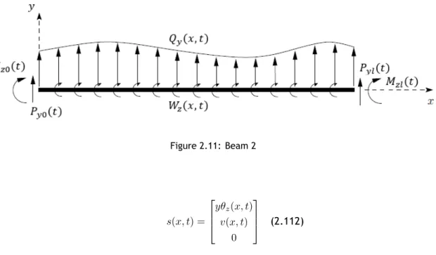
By looking to Figure 2.11 the present loads in this case are:
1. distributed load aligned with y-axis Qy;
2. distributed bending moment Wz;
3. concentrated loads aligned with y-axis Py, one at each beam tip;
Figure 2.11: Beam 2 s(x, t) = yθz(x, t) v(x, t) 0 (2.112)
It is considered that: γxy = γxz = 0the cross section is small when compared with the length
so:
θz=−
∂v
∂x (2.113)
And replacing 2.113 in Equation 2.112 the displacements vector is:
s(x, t) = −y∂v ∂x 0 0 (2.114) ε = −y∂2v ∂x2 0 0 (2.115) σ = Cεx= E −y∂2v ∂x2 0 0 (2.116)
Assuming the discretization of the position domain and looking for a single element with two nodes 2.12 it is possible to obtain the approximation function.
Figure 2.12: Beam 2 Displacements
vj−1(t) - displacement of the element left node
vj(t) - displacement of the element right node
θzj−1(t) - displacement of the element left node
θzj(t) - displacement of the element right node
le- length of the element
vj−1is at ξ = 0 and vj is at ξ = 1 θzj−1 is at ξ = 0 and θzj is at ξ = 1 v(ξ, t) = N (ξ)de(t) (2.117) de(t) = v1(t) θz1(t) v2(t) θz2(t) (2.118) N (ξ) = [ 1− 3ξ2+ 2ξ3 le(ξ− 2ξ2+ ξ3) 3ξ2− 2ξ3 le(−ξ2+ ξ3) ] (2.119) dN dξ = [ −6ξ + 6ξ2 l e(1− 4ξ + 3ξ2) 6ξ− 6ξ2 le(−2ξ + 3ξ2) ] (2.120) d2N dξ2 = [ −6 + 12ξ le(−4 + 6ξ) 6 − 12ξ le(−2 + 6ξ) ] (2.121) And finally:
δv(ξ, t) = N (ξ)δdej(t) (2.122)
The final equation of motion is:
δdTe 1 l3 e ∫ 1 0 ∂2N ∂ξ2 T EIzze ∂2N ∂ξ2 dξde= −δdT ele ∫ 1 0 NTmeN dξ ¨de+ δdTele ∫ 1 0 NTQyedξ + δd T e 1 le ∫ 1 0 ∂N ∂ξ T Wzedξ +δdTeN (0)TPy1+ δdTeN (1) TP y2+ δdTe ∂N ∂ξle T Mz1+ δd T e ∂N ∂ξle T Mz2 (2.123)
Or in its compact form:
δdTeKede=−δdTeMed¨e+ δdTeFe (2.124) Ke= EIzze l3 e 12 6le −12 6le 6le 4le2 −6le 2l2e −12 −6le 12 −6le 6le 2le2 −6le 4l2e (2.125) Me= leme 420 156 22lej 54 −13lej 22lej 4l2ej 13lej −3l2ej 54 13lej 156 −22lej −13lej −3l2ej −22lej 4l2ej (2.126) Fe= leQye 2 1 le 6 1 −le 6 + Py1 1 0 0 0 + Py2 0 0 1 0 + Wze le −1 0 1 0 + Mz1 le 0 1 0 0 + Mz2 le 0 0 0 1 (2.127) de= v1 θz1 v2 θz2 (2.128)
2.7
General Problem
The last step is to join the four resultant matrices in one and it is possible to obtain the general matrices for one element with two tip nodes. The main requirement to do this matrix summation is to select an order for the displacements and then respect that order for the displacements, rigidity and loads matrices. The order chosen for this case is: beam 1, beam 2, rod and bar. That
translates in terms of displacements as: w, v, u, θy, θzand θxfor node one and two respectively.
de= w1 v1 u1 θy1 θz1 θx1 w2 v2 u2 θy2 θz2 θx2 (2.129) Fe= leQze 2 + Pz1− Wye le leQye 2 + Py1− Wze le leQxe 2 + Px1 l2 eQze 12 + My1 le le2Qye 12 + Mz1 le leWxe 2 + Mx1 leQze 2 + Pz2+ Wye le leQye 2 + Py2+ Wze le leQxe 2 + Px2 −l2 eQze 12 + My2 le −l2eQye 12 + Mz2 le leWxe 2 + Mx2 (2.130)
K e = 12 E Iy ye l 3 e 0 0 6 E Iy ye l 2 e 0 0 − 12 E Iy ye l 3 e 0 0 6 E Iy ye l 2 e 0 0 0 12 E Iz ze l 3 e 0 0 6 E Iz ze l 2 e 0 0 − 12 E Iz ze l 3 e 0 0 6 E Iz ze l 2 e 0 0 0 E Ae le 0 0 0 0 0 − E Ae le 0 0 0 6 E Iy ye l 2 e 0 0 4 E Iy ye le 0 0 − 6 E Iy ye l 2 e 0 0 2 E Iy ye le 0 0 0 6 E Iz ze l 2 e 0 0 4 E Iz ze le 0 0 − 6 E Iz ze l 2 e 0 0 2 E Iz ze le 0 0 0 0 0 0 GJ e le 0 0 0 0 0 − GJ e le − 12 E Iy ye l 3 e 0 0 − 6 E Iy ye l 2 e 0 0 12 E Iy ye l 3 e 0 0 − 6 E Iy ye l 2 e 0 0 0 − 12 E Iz ze l 3 e 0 0 − 6 E Iz ze l 2 e 0 0 12 E Iz ze l 3 e 0 0 − 6 E Iz ze l 2 e 0 0 0 − E Ae le 0 0 0 0 0 E Ae le 0 0 0 6 E Iy ye l 2 e 0 0 2 E Iy ye le 0 0 − 6 E Iy ye l 2 e 0 0 4 E Iy ye le 0 0 0 6 E Iz ze l 2 e 0 0 2 E Iz ze le 0 0 − 6 E Iz ze l 2 e 0 0 4 E Iz ze le 0 0 0 0 0 0 − GJ e le 0 0 0 0 0 GJ e le (2.131)
M e = 156 le m e 420 0 0 22 l 2me e 420 0 0 54 le m e 420 0 0 − 13 l 2me e 420 0 0 0 12 156 le m e 420 0 0 22 l 2me e 420 0 0 54 le m e 420 0 0 − 13 l 2me e 420 0 0 0 2 le m e 6 0 0 0 0 0 le m e 6 0 0 0 22 l 2me e 420 0 0 4 l 3me e 420 0 0 13 l 2me e 420 0 0 − 3 l 3me e 420 0 0 0 22 l 2me e 420 0 0 4 l 3me e 420 0 0 13 l 2me e 420 0 0 − 3 l 3me e 420 0 0 0 0 0 0 2 le Ip e 6 0 0 0 0 0 le Ip e 6 54 le m e 420 0 0 13 l 2me e 420 0 0 156 le m e 420 0 0 − 22 l 2me e 420 0 0 0 54 le m e 420 0 0 13 l 2me e 420 0 0 156 le m e 420 0 0 − 22 l 2me e 420 0 0 0 le m e 6 0 0 0 0 0 2 le m e 6 0 0 0 − 13 l 2me e 420 0 0 − 3 l 3me e 420 0 0 − 22 l 2me e 420 0 0 4 l 3me e 420 0 0 0 − 13 l 2me e 420 0 0 − 3 l 3me e 420 0 0 − 22 l 2me e 420 0 0 4 l 3me e 420 0 0 0 0 0 0 le Ip e 6 0 0 0 0 0 2 le Ip e 6 (2.132)
The general problem allows the computation in a 3D space of structures that may not be aligned with the x-axis as the FEM formulation was developed. So, it is first required to perform a space rotation to ensure that the general reference axes are coherent. This rotation is done using the matrix 2.133 where A represents the matrix with the transformation using the three possible
rotation angles: ϕhe, ϕveand ϕxefor each element as Figure 2.13 shows, and B is a zeros matrix.
rote= A B B B B A B B B B A B B B B A (2.133) A =
cos ϕhe× cos ϕve cos ϕxe× sin ϕhe sin ϕhe× sin ϕxe
− cos ϕhe× sin ϕve× sin ϕxe + cos ϕhe× cos ϕxe× sin ϕve
− cos ϕve× sin ϕhe cos ϕhe× cos ϕxe cos ϕhe× sin ϕxe
+ sin ϕhe× sin ϕve× sin ϕxe − cos ϕxe× sin ϕhe× sin ϕve
− sin ϕve − cos ϕve× sin ϕxe cos ϕve× cos ϕxe
(2.134) B = 0 0 0 0 0 0 0 0 0 (2.135)
Figure 2.13: Rotation Angles.
rotation matrix 2.133. The loads matrix does not require this step because the loads are initially inserted assuming the general reference axis.
Ke= rotTe × Ke× rote (2.136)
Me= rotTe × Me× rote (2.137)
Fe= rotTe × Fe (2.138)
The last step before the computation of the displacements is to assemble the general matrices for the structure, those matrices contain now all the mesh elements. After assuming an order for the global nodes in the final matrices the principle is to sum, in the correct position of this matrix, the equal degrees of freedom of the nodes of each individual element matrix. If there is not any global node in more than two elements and the nodes are ordered consecutively this step can be done as Figure 2.14 shows, in which each X represents the six DOF of one node.
Figure 2.14: Matrices Assembly.
Once having those matrices, the structural displacements problem 2.139 can be solved using methods like: elimination of variables, Cramer’s rule or row reduction (also known as Gaussian elimination). In this code the Gauss elimination method is used. The natural frequency free vibrations are calculated using by calculating the eigenvalues ω of the equation 2.140 and the eigenvectors ν. Linear Algebra Package (LAPACK) is a software library that is applied in the code
to solve the two solutions.
K× d = F (2.139)
Chapter 3
Code Development
3.1
Code Structure
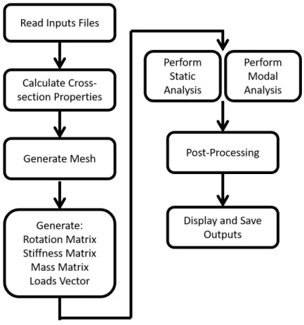
This chapter shows how to apply the mathematical model to a computer code. The code should have a simple and clear structure, like Figure 3.1, to avoid errors and allow future developments. So, the current code is divided into the following items:
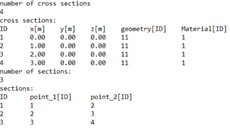
1. Input data:
(a) Section geometry; (b) Material properties; (c) Loads;
(d) Boundary conditions; (e) Structure shape. 2. Section geometry:
(a) Section properties (section 3.3). 3. Generate mesh;
4. Generate stiffness matrix; 5. Generate mass matrix; 6. Generate rotation matrix; 7. Apply loads in the mesh nodes; 8. Generate loads vector;
9. Apply the problem boundary conditions to the loads and displacements vectors; 10. Perform static analysis to determine the structure displacements;
11. Perform modal analysis to determine the free vibration modes; 12. Show the displaced mesh and structure;
13. Show results.
As it is possible to see in Figure 3.1 the tasks above follow an order that the code must respect to be able to perform a correct analysis.
![Figure 2.2: Historical Evolution of the FEM [OCZ00].](https://thumb-eu.123doks.com/thumbv2/123dok_br/18041799.862223/28.892.116.737.496.906/figure-historical-evolution-of-the-fem-ocz.webp)
![Figure 2.3: Algorithm for a FEM Analysis [Bat14].](https://thumb-eu.123doks.com/thumbv2/123dok_br/18041799.862223/29.892.293.650.447.876/figure-algorithm-for-a-fem-analysis-bat.webp)