doi:10.5194/amt-9-2345-2016
© Author(s) 2016. CC Attribution 3.0 License.
Evaluation of multifrequency range imaging technique implemented
on the Chung–Li VHF atmospheric radar
Jenn-Shyong Chen1, Shih-Chiao Tsai2, Ching-Lun Su3, and Yen-Hsyang Chu3 1Center for General Education, China Medical University, Taichung, Taiwan
2Department of Environmental Information and Engineering, National Defense University, Taoyuan, Taiwan 3Graduate Institute of Space Science, National Central University, Taoyuan, Taiwan
Correspondence to:Jenn-Shyong Chen ([email protected])
Received: 19 August 2015 – Published in Atmos. Meas. Tech. Discuss.: 29 September 2015 Revised: 24 April 2016 – Accepted: 1 May 2016 – Published: 27 May 2016
Abstract. The multifrequency range imaging tech-nique (RIM) has been implemented on the Chung–Li VHF array radar since 2008 after its renovation. This study made a more complete examination and evaluation of the RIM technique to facilitate the performance of the radar for atmospheric studies. RIM experiments with various radar parameters such as pulse length, pulse shape, receiver bandwidth, transmitter frequency set, and so on were conducted. The radar data employed for the study were collected from 2008 to 2013. It has been shown that two factors, the range/time delay of the signal traveling in the media and the standard deviation of Gaussian-shaped range-weighting function, play crucial roles in ameliorating the RIM-produced brightness (or power distribution); the two factors are associated with some radar parameters and system characteristics. The range/time delay of the signal was found to increase with time; moreover, it was slightly different for the echoes from the atmosphere with and with-out the presence of significant precipitation. A procedure of point-by-point correction of range/time delay was thus exe-cuted for the presence of precipitation to minimize the bogus brightness discontinuity at range gate boundaries. With the RIM technique, the Chung–Li VHF radar demonstrates its first successful observation of double-layer structures as well as their temporal and spatial variations with time.
1 Introduction
The mesosphere–stratosphere–troposphere (MST) radar op-erated at very-high-frequency (VHF) band is a powerful in-strument to study the atmosphere from near the ground up to the ionosphere. Among the capabilities of VHF-MST radar, continuous measurement of three-dimensional winds with a temporal resolution of several minutes and a vertical resolu-tion of several hundred meters are praiseworthy (Lee et al., 2014). In addition to the air motion characterized by the wind field, small-scale structures of refractivity irregularities, such as thin layers with a thickness of tens of meters, exist com-monly in the atmosphere and can reflect dynamic behavior of the atmosphere directly. However, a conventional atmo-sphere radar that operates at a specific frequency and a finite pulse length is unable to resolve the thin-layer structures em-bedded within the range gate. In view of this, a frequency-hopped technique was introduced to the pulsed radar to over-come this limitation (Franke, 1990). The frequency-hopped technique was initially implemented with two frequencies on the VHF-MST radar, which can only resolve a Gaussian-shaped single layer in the range gate. Implementation of the frequency-hopped technique with more than two fre-quencies was not achieved until 2001 for an ultra-high-frequency (UHF) wind profiler (Platteville 915 MHz radar at 40.19◦N, 104.73◦W) (Chilson et al., 2003, 2004). Since
then, the European Incoherent Scatter (EISCAT) VHF radar, the Middle and Upper Atmosphere Radar (MUR; 34.85◦N,
136.10◦E), the Ostsee Wind (OSWIN) VHF radar (54.1◦N,
11.8◦E), the Chung–Li VHF radar (24.9◦N, 121.1◦E), and
grav-2346 J.-S. Chen et al.: Evaluation of multifrequency range imaging technique
ity waves, double-layer structures, Kelvin–Helmholtz insta-bility (KHI) billows, convective structures, polar mesosphere summer echoes (PMSE), and so on, with high resolution in the range direction (e.g., Fernandez et al., 2005; Luce et al., 2006, 2008; Chen and Zecha, 2009; Chen et al., 2009). The terminologies of range imaging (RIM) (Palmer et al., 1999) and frequency interferometric imaging (FII) (Luce et al., 2001) were given to the frequency-hopped technique for the radar remote sensing of the atmosphere. Some advanced applications of RIM have also been proposed, e.g., a high-resolution measurement of wind field in the sampling gate (Yu and Brown, 2004; Chilson et al., 2004; Yamamoto et al., 2014). Moreover, three-dimensional imaging of the scatter-ing structure in the radar volume has been put into practice by combining RIM and coherent radar imaging (CRI) tech-niques (Hassenpflug et al., 2008; Chen et al., 2014a). Re-cently, some efforts on the calibration process of radar echoes were made to improve the performance of RIM (Chen et al., 2014b). In addition to the aforementioned works of RIM, a deconvolution procedure working with a swept-frequency pulse has been employed (Hocking et al., 2014), which also provided a range resolution higher than the pulse-defined value.
In this study, a large amount of RIM data that were col-lected by the Chung–Li VHF radar with various pulse lengths and shapes, phase codes, receiver bandwidths, frequency sets, and so on for the period from 2008 to 2013 were an-alyzed to evaluate the capability of the RIM technique im-plemented on the radar. It has been shown that the perfor-mance of RIM for the thin-layer measurement relies on a proper calibration of the radar data, including time delay of radar signal, signal-to-noise ratio (SNR), and the range-weighting function effect (Chen and Zecha, 2009). The time delay of the radar signal traveling in the media – such as the cable lines, free space, and processing time in the radar system – leads to a range delay and thereby gives a range error in the RIM processing. Furthermore, the removal of the range-weighting function effect on the spatial distribu-tion of the RIM-produced brightness is required to restore the finer structures in the radar volume (Chen et al., 2014b). To this end, the calibration approach proposed by Chen and Zecha (2009), which is more convenient for our analysis, was employed in this study.
This article is organized as follow. In Sect. 2, the RIM capability of the Chung–Li VHF radar is introduced briefly. Section 3 gives an example of RIM as well as its calibration results for different radar parameters such as receiver sys-tem and frequency set. Section 4 presents the observations of precipitation and some layer structures. It is found that the time delay measured for precipitation echoes was different slightly from that of clear-air turbulences. A deeper exam-ination was made to improve the RIM-produced brightness for precipitation echoes. In addition, double-layer structures and finer parts within the structures were resolved
success-fully to demonstrate the capability of RIM implemented on the radar system. Conclusions are drawn in Sect. 5.
2 Range imaging technique of the Chung–Li VHF radar
The Chung–Li VHF radar system, operated at a central fre-quency of 52 MHz, has been upgraded for several years and carried out some valuable studies for the atmosphere (Chu et al., 2013; Su et al., 2014). In addition to a great improvement in radar signal processing, various pulse shapes such as rect-angular, Gaussian, and trapezoid are available, and typical pulse widths are 1, 2, and 4 µs, yielding range gate resolu-tions of 150, 300, and 600 m, respectively. In addition, the range step can be as small as 50 m for oversampling (Chen et al., 2014b). Corresponding filter bandwidths can be cho-sen to match the transmitted pulse widths and pulse shapes. Barker and complementary codes are available to raise the signal-to-noise ratio of the received echoes, and more than five frequencies with a frequency step as small as 1 Hz can be set. These renovations and improvements in the radar char-acteristics enable the newly upgraded Chung–Li VHF radar to use the RIM technique to observe finer structures in the at-mosphere. The first RIM experiment made with the Chung– Li radar was conducted successfully in 2008 (Chen et al., 2009), and since then plenty of experiments with the RIM mode have been carried out by the radar. Table 1 lists many of the observations and their calibration results that will be discussed later. As listed, 1 and 2 µs pulse lengths, three types of pulse shapes, and different bandwidths and frequency sets were tested. Moreover, three receiving channels (subarrays) were operated for reception of radar echoes. The analysis of various kinds of radar data can help us to realize the capa-bility of the RIM technique implemented on the radar sys-tem for atmospheric measurements. A possible drawback of RIM may arise from the relatively broad radar beamwidth (∼7.4◦), which smears the measured structure imaging due
to a noticeable curvature of the radar beam.
for the atmosphere, however, the number of carrier frequen-cies is limited, which will be discussed in Sect. 3.3. In addi-tion, it is supposed that the principal layers or targets in the range gate interval (commonly from 150 to 600 m) are less than two or three. Therefore, the requirement of a large num-ber of carrier frequencies can be discarded, and the Capon method is still sufficient for use with a smaller number of carrier frequencies, say, four or five.
To acquire proper imaging of refractivity structures, cor-rections of range error and range-weighting function effect are essential. In this study, we employed the calibration ap-proach given by Chen and Zecha (2009) to make neces-sary corrections, which has been successfully tested for the Chung–Li radar and the MUR (Chen et al., 2009). The es-timator of mean square error that is used to determine the optimal parameters for correcting the RIM-produced bright-ness is given by
1B=
N
X
i=1
(B1i−B2i)2
B1iB2i
, (1)
whereB1i andB2i are two sets of RIM-produced brightness
values in the overlapped sampling range intervals of two ad-jacent range gates. N is the number of brightness values. Although the echoing structures in the overlapped sampling range intervals are the same and are supposed to have similar
B1andB2values, the estimatedB1andB2values may not be close to each other owing to two factors: sampling range error and range-weighting effect. Therefore,B1andB2values are expected to approximate to each other after the two factors are mitigated. In the calibration process, the optimal mitiga-tion of the two factors gives the smallest value of1B, which is achieved by changing iteratively the sampling range er-ror and the standard deviation of the Gaussian-shaped range-weighting function in computing.
3 Observations and calibrations
Table 1 lists 16 cases of RIM experiments that were carried out between 2008 and 2013 by using the Chung–Li VHF radar. With the plentiful radar data, the long-term variation in some of the characteristics of radar system will be addressed and discussed. In addition, the RIM experiments conducted on 9 November 2009 (cases 9 and 10) are presented as typical cases for specific demonstration in the following.
3.1 Different receiver systems
Figure 1 shows the statistical results of the calibration-estimated phase bias (left panels) and standard deviation
σz (right panels) of the Gaussian range-weighting function
exp(−r2/σz2), wherer is the range relative to the gate cen-ter, for the radar data of case 10. Only the atmospheric echoes with the SNR larger than −9 dB were analyzed and are presented in Fig. 1. Note that the phase bias is a
0 20 40
720 1080 1440
Phase bias vs. SNR
SNR (dB)
Phase bias (deg)
0 20 40
50 150 250 350
σ
z vs. SNR
SNR (dB)
σz
(m)
0.01995 −0.02188 0.2 0 (b)
Figure 1: (a) Histograms of the calibrated parameters for three independent
receiving channels. Phase bin is 20
oand
z
bin is 10 m. The shapes and sizes of the
three receiving arrays are the same. (b) Scatter plot of the calibrated parameters vs.
SNR for the second receiving channel (Rx_2). The curve describing the relationship
between
zand SNR is a fitting curve for correcting the RIM-produced brightness.
Data time: 06:49:27 UT – 08:49:47 UT, 9 November 2009.
720 1080 14400 0.5 1
Histogram of phase bias
Phase bias (deg)
Normalized number
50 150 250 350 0
0.5 1
Histogram of σ z
σ z (m)
720 1080 1440 0
0.5 1
Histogram of phase bias
Phase bias (deg)
Normalized number
50 150 250 350 0
0.5 1
Histogram of σ
z
σ
z (m)
720 1080 1440 0
0.5 1
Histogram of phase bias
Phase bias (deg)
Normalized number
50 150 250 350 0
0.5 1
Histogram of σ z
σ z (m) Rx_1
Rx_2
Rx_3 (a)
Figure 1. (a)Histograms of the calibrated parameters for three
in-dependent receiving channels. Phase bin is 20◦, andσzbin is 10 m. The shapes and sizes of the three receiving arrays are the same. (b)Scatterplot of the calibrated parameters vs. SNR for the sec-ond receiving channel (Rx_2). The curve describing the relation-ship betweenσzand SNR is a fitting curve for correcting the RIM-produced brightness. Data time: 06:49:27–08:49:47 UT, 9 Novem-ber 2009.
value transformed from the following equation: range de-lay×360◦/ range gate interval. Therefore, in this case the
phase bias of 360◦corresponds to a range delay of 150 m or
a time delay of 0.5 µs for the signal propagation.
As shown in Fig. 1, the phase bias histograms of the three receiving channels were consistent with each other. The mean phase biases were centered at around 1230◦(peak
2348 J.-S. Chen et al.: Evaluation of multifrequency range imaging technique
In view of this, the three receiver systems are thought to be approximately identical in conducting the RIM experiment. This, however, does not mean that the system phase differ-ence between receiving channels, which is a crucial parame-ter for spatial radar inparame-terferometry, is close to zero. Similarity of phase bias distributions between different receiving chan-nels suggests that the range/time delay is not the main cause of the system phase difference, if one exists, between receiv-ing channels of the Chung–Li radar. This issue needs to be clarified by other means and will not be discussed further in this study.
Figure 1b presents scatter diagrams of phase bias (left) and
σz(right) vs. SNR. As shown, for the data with SNR > 0 dB,
the phase biases are distributed mainly in a range of 1080– 1440◦, centered at around 1230◦. By contrast, theσzvalues
were SNR dependent, as seen in the right panel of Fig. 1b. A curve has been determined to represent the relationship be-tweenσzand SNR (Chen and Zecha, 2009), which is
benefi-cial to produce the structure at gate boundaries with smoother imaging and is given below:
σz=
1
a
(SNR+10)C +b
−d, (2)
where the four constants a, b, c, and d are given in the plot (reading from top to bottom). The fitting curve reveals that the σz value tended to approach a constant value of
about 100 m as the SNR increased. This curve-approached
σz value at high SNR was close to the peak location ofσz
histogram (∼115 m) shown in the right panels of Fig. 1a. The σz value at large SNR or the peak location of the σz
histogram can describe the theoretical shape of the Gaussian range-weighting function. As derived in the previous studies (e.g., Franke, 1990), the standard deviation of the Gaussian range-weighting function is given by 0.35cτ/ 2, wherecis the speed of the light andτ is the pulse width. This value is obtained for a rectangular pulse shape used with its matched filter; for example, 52.5 m for 1 µs pulse width. According to our definition of Gaussian range-weighting function, how-ever,σzequals
√
2×0.35cτ/2, namely, about 74 m for 1 µs pulse width. This number is smaller than the calibrated value (100 or 115 m). This is because the case presented in Fig. 1 employed a Gaussian instead of rectangular pulse shape, re-sulting in a range-weighting function broader than that de-fined by the standard deviation of 74 m. By contrast, a trape-zoid pulse shape that is close to a rectangular shape was em-ployed in case 8, thereby resulting in a value of 80 m for the peak location ofσz, which is not far from the value of 74 m.
As for the dependence of theσz value on SNR, it is not
un-accountable because the performance of the Capon method is also SNR-dependent (Palmer et al., 1999; Yu and Palmer, 2001). As the SNR decreases, the RIM brightness becomes less accurate. In addition, there should be less and less to im-age as the SNR gets lower. As a result, the range-weighting effect becomes unimportant and a larger value of σz is
ob-tained from the calibration process for a lower SNR case. It
0 0.5 1 1.5 2 2.5
1 2 3 4 5 6 7 8 9 10 11 12 13 14 15 16
Ti
m
e
de
la
y
(
s)
Cases Time delay for Rx_1
(2009/07‐11)
(2011/12) (2012/01) (2012/08)
(2008/03‐09)
(2013/08)
1 s
2 s
Figure 2: Time delays in different time periods. Refer to Table 1 for the observational
time period of each case.
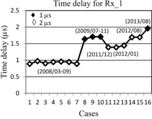
Figure 2.Time delays in different time periods. Refer to Table 1 for
the observational time period of each case.
should be recalled that the relationship curve forσzand SNR
could vary with the optimization method of range imaging; the calibration results exhibited in this paper are valid only for the Capon method.
3.2 Time- and radar-parameter-dependent characteristics
As revealed in Table 1, the peak location of phase bias varied with time. For 1 µs pulse length, the peak location was larger in 2013 than in 2009. For 2 µs pulse length the peak loca-tions obtained in 2011 and 2012 were evidently larger than those obtained in 2008. The increase in phase bias with time is presumably due to the aging of cable lines or some com-ponents in the radar system that cause additional time delay of signal. As shown in Fig. 2, the time delay estimated from the phase bias of receiver 1 (Rx_1) indeed has a tendency to increase with time. Nevertheless, those values of time delays for 1 µs pulse length in 2009 were obviously larger than the level indicated by the increasing tendency of time delay. It is thus worthy of additional investigation in the future to learn whether the radar system responds to different pulse lengths to result in various time delays; this can provide us a fully un-derstanding of the characteristics of the radar system or other fundamental factors.
On the other hand, the peak location of theσz histogram,
σz,peak, was not time dependent. Instead, it is a function of pulse shape and filter bandwidth, for example, the three radar experiments (cases 2–4) conducted on 11 April 2008 with different pulse shapes and filter bandwidths that were set al-ternately in the experiments (Chen et al., 2009). The exper-iment with Gaussian-shaped pulse and 250 kHz bandwidth (case 2) had a largerσz,peak than that with squared pulse shape but the same filter bandwidth (case 3), and also larger than that with the same pulse shape but 500 kHz bandwidth (case 4), indicating a dependence ofσzvalue on radar pulse
shape as well as receiver bandwidth.
Table 1.RIM experiments of the Chung–Li VHF radar and calibration results.
Case Exp. date Pulse length (µs)/ Filter band- Freq Sampling Calibration results:
(hh:mm, UT) shape/code or width (kHz) set (MHz)/ time (s) peak location of phase bias/σz,peak
oversampling freq. no. range delay/time delay
Rx_1 Rx_2 Rx_3
1 2008/03/30 2/s 500 fa/5 0.256 320◦/160 m 320◦/180 m 330◦/170 m
(17:05–24:00) (267 m/0.889 µs)
2 2008/04/11a 2/g 250 fa/5 0.256 350◦/260 m 340◦/250 m 350◦/260 m
(02:50–04:20) (292 m/0.972µs)
3 2008/04/11b 2/s 250 fa/5 0.256 325◦/210 m 340◦/200 m 330◦/210 m
(02:50–04:20) (271 m/0.903 µs)
4 2008/04/11c 2/g 500 fa/5 0.256 340◦/210 m 350◦/210 m 350◦/220 m
(02:50–04:20) (283 m/0.944 µs)
5 2008/09/12a 2/s 250 fa/5 0.256 345◦/220 m 350◦/220 m 350◦/220 m
(02:54–05:17) (288 m/0.958 µs)
6 2008/09/12b 2/s 250 fb/5 0.256 340◦/220 m 350◦/225 m 350◦/220 m
(02:54–05:17) (283 m/0.944 µs)
7 2008/09/12c 2/s/7 bit Barker 500 fa/5 0.32 320◦/180 m 315◦/160 m 320◦/170 m
(06:12–07:15) (267 m/0.889 µs)
8 2009/07/27 1/T 1000 fd/5 0.512 1180◦/80 m 1180◦/85 m 1200◦/80 m
(05:30–08:23) (492 m/1.639 µs)
9 2009/11/09a 1/g 1000 fe/7 0.1792 1230◦/115 m 1230◦/115 m 1250◦/115 m
(03:08–05:38) (513 m/1.708 µs)
10 2009/11/09b 1/g 1000 ff/7 0.1792 1230◦/115 m 1230◦/115 m 1240◦/120 m
(06:49–08:49) (513 m/1.708 µs)
11 2011/12/02 2/g/over 500 fa/5 0.128 500◦/210 m 505◦/200 m 505◦/200 m
(03:39–05:52) (417 m/1.389 µs)
12 2012/01/05 2/s/over 500 fa/5 0.128 500◦/150 m 500◦/150 m 500◦/150 m
(02:22–04:56) (417 m/1.389 µs)
13 2012/01/05 2/s/over 1000 fa/5 0.128 520◦/135 m 520◦/140 m 530◦/140 m
(04:59–07:38) (433 m/1.444 µs)
14 2012/08/08a 2/s/over 500 fc/7 0.1792 610◦/160 m 620◦/160 m 615◦/160 m
(05:32–07:02) (508 m/1.694 µs)
15 2012/08/08b 2/s/over 500 fg/7 0.1792 610◦/150 m 615◦/160 m 615◦/150 m
(07:07–08:37) (508 m/1.694 µs)
16 2013/08/21 1/g 1000 fd/5 0.128 1410◦/110 m 1420◦/110 m 1410◦/110 m
(00:00–07:00) 586 m/1.958 µs)
fa: 51.75, 51.875, 52.0, 52.125, 52.25;fb: 51.75, 51.8, 52.0, 52.1, 52.25;fc: 51.75, 51.8, 51.875, 52.0, 52.1, 52.125, 52.25;fd: 51.5, 51.75, 52, 52.25, 52.5;fe: 51.5, 51.6, 51.75,
52.0, 52.2, 52.25, 52.5;ff: 51.5, 51.75, 51.875, 52, 52.125, 52.25, 52.5;fg: 51.75, 51.833334, 51.916667, 52.0, 52.083333, 52.166666, 52.25; pulse shape: g≡Gaussian, s≡square, T≡trapezoid; over: oversampling with a range step of 50 m.
and filter bandwidth employed in the three experiments were the same, but the frequency sets and the pulse shapes were different. The trapezoid shape employed in case 8 is a mod-ified square pulse with a suppression of the sharp slopes at rising and falling edges of the pulse. We shall show later that the number of frequencies was not the main cause of varia-tion inσz,peakwhen the number of frequencies was more than five. On the other hand, the pulse shape plays a role in deter-mining theσz,peakvalue, in which the trapezoid pulse shape
resulted in a smaller value ofσz,peak. In addition, the peak location of phase bias on 27 July (case 8) was smaller than that on 9 November (cases 9 and 10) by about 50◦; again, we
attribute it to the aging of cable lines or some components in the radar system.
no-2350 J.-S. Chen et al.: Evaluation of multifrequency range imaging technique
720 1080 1440 0
0.5 1
Histogram of phase bias
Phase bias (deg)
Normalized number
50 150 250 350 0
0.5 1
Histogram of σ
z
σ
z (m)
720 1080 1440 0
0.5 1
Histogram of phase bias
Phase bias (deg)
Normalized number
50 150 250 350 0
0.5 1
Histogram of σ
z
σ
z (m)
720 1080 1440 0
0.5 1
Histogram of phase bias
Phase bias (deg)
Normalized number
50 150 250 350 0
0.5 1
Histogram of σ
z
σ
z (m)
720 1080 1440 0
0.5 1
Histogram of phase bias
Phase bias (deg)
Normalized number
50 150 250 350 0
0.5 1
Histogram of σ
z
σ
z (m)
720 1080 1440 0
0.5 1
Histogram of phase bias
Phase bias (deg)
Normalized number
50 150 250 350 0
0.5 1
Histogram of σ
z
σ
z (m)
720 1080 1440 0
0.5 1
Histogram of phase bias
Phase bias (deg)
Normalized number
50 150 250 350 0
0.5 1
Histogram of σ
z
σ
z (m)
720 1080 1440 0
0.5 1
Histogram of phase bias
Phase bias (deg)
Normalized number
50 150 250 350 0
0.5 1
Histogram of σ
z
σ
z (m)
720 1080 1440 0
0.5 1
Histogram of phase bias
Phase bias (deg)
Normalized number
50 150 250 350 0
0.5 1
Histogram of σ
z
σ
z (m)
720 1080 1440 0
0.5 1
Histogram of phase bias
Phase bias (deg)
Normalized number
50 150 250 350 0
0.5 1
Histogram of σ
z
σ
z (m)
720 1080 1440 0
0.5 1
Histogram of phase bias
Phase bias (deg)
Normalized number
50 150 250 350 0
0.5 1
Histogram of σ
z
σ
z (m)
(a) Two frequencies (b) Three frequencies
(c) Five frequencies (d) Seven frequencies
Figure 2.
Histograms of the calibrated parameters for different sets of transmitter
frequencies, with the radar data collected from the second receiving channel (Rx_2) in
Fig. 1. The values quoted at the title locations are the transmitter frequencies; the unit
is MHz.
(51.5, 52.5)
(51.75, 52.25)
(51.875, 52.125)
(52.0, 52.125)
(51.75, 52.0, 52.25)
(51.875, 52.0, 52.125) (51.5, 52.0, 52.5)
(51.5, 51.75, 52.0, 52.25, 52.5)
(51.75, 51.875, 52.0, 52.125, 52.25)
(51.5, 51.75, 51.875, 52.0, 52.125, 52.25, 52.5)
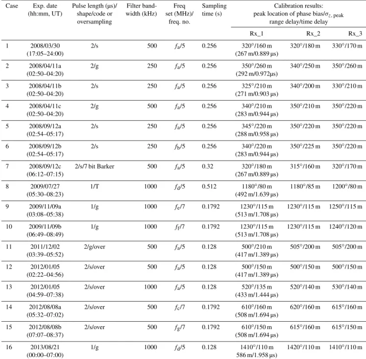
Figure 3.Histograms of the calibrated parameters for different sets of transmitter frequencies, with the radar data collected from the second
receiving channel (Rx_2) in Fig. 1. The values quoted at the title locations are the transmitter frequencies; the unit is MHz.
ticeable differences in the calibration results between the two cases. Moreover, the radar system was stable in 2008 because the peak locations of phase biases were in general agreement with each other.
3.3 Different frequency sets
RIM exploits an advantage of frequency diversity. The num-ber of carrier frequencies and the frequency step play cru-cial roles in determining the performance of RIM. Neverthe-less, the number of carrier frequencies used in the experiment is subject to the radar parameters and target characteristics both. One of the assumptions of RIM is that the targets do not change their locations and characteristics during a cycle
of carrier frequency set. When the target varies rapidly, the sampling time must be short enough, meaning the IPP should be short or the number of carrier frequencies cannot be too large. In all experiments listed in Table 1, the sampling times were sufficiently shorter than the variation timescale of the atmospheric targets (∼1 s), satisfying the basic assumption of invariant targets for RIM.
Figure 3 compares the histograms of the calibration-estimated phase biases andσzvalues at different frequency
7 7.2 7.4 7.6 7.8 8 8.2 8.4 8.6 8.8 2
3 4 5 6 7
UT (h)
Range height (km)
0 10 20 30 40 50 60 70
3.5 4 4.5 5 5.5
2 3 4 5 6 7
UT (h)
Range height (km)
0 10 20 30 40 50 60 70
(a) Height–time–intensity Range-imaging brightness (dB)
(b) Height–time–intensity Range-imaging brightness (dB)
Figure 3: (a) (Left) High-time intensity with a range resolution of 150 m, and (right) range imaging with a range step of 1 m. (b) is similar to (a), but the radar data were collected later on the same day (9 November 2009).
Figure 4. (a)(Left) Height–time–intensity with a range resolution of 150 m, and (right) range imaging with a range step of 1 m.(b)is similar
to(a), but the radar data were collected later on the same day (9 November 2009).
clearly demonstrates that our calibration process is a robust approach to estimate the range/time delay of signal in the media and/or radar system. It can also be seen from Fig. 3 that the more the carrier frequency number is used, and the smaller the frequency separation is given, the more concen-trated the distributions of phase biases andσzvalues will be.
A closer examination shows that the peak locations ofσz
his-tograms approximate to a value of 120 m as the number of carrier frequencies increases.
In light of the fact that the performance of estimating the phase bias and theσzvalue is superior with more carrier
fre-quencies and a smaller frequency step, we exhibit the RIM results of cases 9 and 10 to demonstrate finer atmospheric layer structures within the range gates, as shown in Fig. 4. The left panels of Fig. 4 shows the original height time-intensity (HTI) plots with a range resolution of 150 m, and the right panels displays the RIM-produced brightness dis-tributions with an imaging step of 1 m. In Fig. 4, there were
2352 J.-S. Chen et al.: Evaluation of multifrequency range imaging technique
5 5.2 5.4 5.6 5.8 6
2 3 4 5 6 7
UT (h)
Range (km)
0 10 20 30 40 50 60 70 80
(dB)
Figure 4: (a) High-time intensity with a range resolution of 150 m, and (b, c)
RIM-produced brightness with, respectively, constant and adaptive values of range
error in the correction process. Imaging range step is 1 m. Data time: 21 August 2013.
(b) RIM with constant phase bias (a) Height–time–intensity (21 Aug 2013)
(c) RIM with adaptable phase bias
Range
height
(k
m
)
Range
height
(k
m
)
Range
height
(k
m
)
Figure 5.(upper) Height–time–intensity with a range resolution of
150 m, and (middle and bottom) RIM-produced brightness with, re-spectively, constant and adaptive values of range error in the cor-rection process. Imaging range step is 1 m. Data time: 21 August 2013.
4 More observations and discussion 4.1 RIM for precipitation echoes
The calibration approach employed in the preceding section for RIM is based on the assumption that the atmospheric structures are continuous at the common edges of two
ad-4.9 5.1 5.3 5.5 5.7 5.9 6.1
0 50 100
2013/08/21 Disdrometer
UT (h)
Rainrate (mm h )
velocity (m s )
Height(km)
2013−08−21 5−18−17
−10 0 10
2 3 4 5 6 7
dB
0 10 20 30 40 50 60
Height(km)
2013−08−21 5−34−40
−10 0 10
2 3 4 5 6 7
dB
10 20 30 40 50
Height(km)
2013−08−21 5−59−22
−10 0 10
2 3 4 5 6 7
dB
10 20 30 40 50 60
(a)Rain rate
(b)Power spectra of radar echoes
Figure 5: (a) Rain rate measured by the disdrometer located near the radar site. (b) Three typical power spectra of radar echoes at the times indicated sequentially by the red arrows in (a).
–1
– 1
velocity (m s )– 1 velocity (m s )– 1
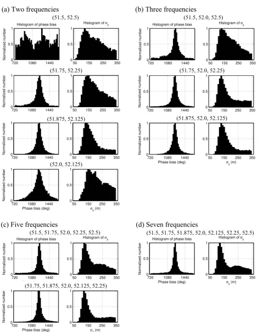
Figure 6. (a)Rain rate measured by the disdrometer located near
the radar site.(b)Three typical power spectra of radar echoes at the times indicated sequentially by the red arrows in(a).
through-out the altitude range; it is clear that the echoes were gen-erated by refractivity fluctuations without the contribution from precipitation particles. By contrast, Doppler velocities with large negative values were observed in the middle panel, which were associated with heavy rain. Note that the rainfall velocity was so large that Doppler aliasing happened. The leftmost panel shows the condition of moderate precipitation, in which the spectral power of precipitation was much lower than that of refractivity fluctuations.
After range imaging with the constant phase bias indicated in Table 1, the RIM-produced brightness in the middle panel of Fig. 5 exhibits evident discontinuities at the boundaries of range gates in the periods when intense precipitation oc-curred. This feature is presumably due to improper phase bias (range error) compensating in the RIM processing. When adaptable phase bias was adopted for each estimate of bright-ness, we obtained a better result as shown in the lowest panel of Fig. 5. As seen, discontinuity of the RIM-produced bright-ness through gate boundaries has been mitigated for precipi-tation echoes. In the following, we illustrate the necessity of using adaptable phase bias for precipitation echoes.
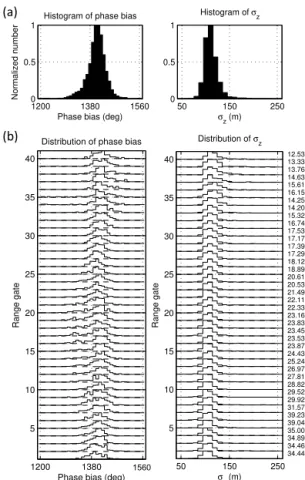
Figure 7a shows the histograms of phase biases andσz
val-ues for the data presented in Fig. 5. The overall features of the histograms of phase biases and σz values are similar to
those shown in Fig. 1, except for the peak location of phase biases. Normalized distributions of phase biases andσz
val-ues varying with range gates are shown in panel b. In gen-eral, the phase biases are centered at around 1400◦.
How-ever, some phase biases with values smaller than 1400◦ by
as far as 90◦can be observed in the range interval between
the 11th and 25th range gates. An examination shows that these phase biases were associated with intense precipitation echoes. On the other hand, the distributions ofσzvalues were
quite consistent across all range gates. Accordingly, adapt-able phase bias for correction of range/time error is required to produce a more continuous imaging structure; the result has been shown in the lowest panel of Fig. 5.
The cause of difference in phase bias between precipita-tion and refractivity fluctuaprecipita-tions is still unknown. A plausi-ble conjecture is spatially inhomogeneous distribution and temporally quick change of the discrete-natured precipitation particles in the radar volume, which may lead to a breakdown of the assumptions for calibration of RIM data. This issue may be investigated and clarified by using the technique of multi-receiver CRI (Palmer et al., 2005). Unfortunately, the Chung–Li radar does not have enough receiving channels for CRI technique, and we need other suitable radars with CRI capability to conduct the radar experiment to tackle the prob-lem of difference in phase bias between precipitation and re-fractivity fluctuations.
4.2 Double-layer structures
As shown in Fig. 4, various thin-layer structures can be dis-closed by using the RIM technique. In this sub-section, two
1200 1380 1560 0
0.5 1
Histogram of phase bias
Phase bias (deg)
Normalized number
50 150 250 0
0.5 1
Histogram of σ
z
σ
z (m)
1200 1380 1560 5 10 15 20 25 30 35 40
Distribution of phase bias
Phase bias (deg)
Range gate 34.44 34.46 34.89 35.00 39.04 39.23 31.57 29.92 29.52 28.82 27.81 26.97 25.24 24.43 23.87 23.53 23.45 23.83 23.16 22.33 22.11 21.49 20.53 20.61 18.89 18.12 17.29 17.39 17.17 17.53 16.74 15.32 14.20 14.25 16.15 15.61 14.63 13.76 13.33 12.53
50 150 250 5 10 15 20 25 30 35 40
Distribution of σ
z
σ
z (m)
Range gate 34.44 34.46 34.89 35.00 39.04 39.23 31.57 29.92 29.52 28.82 27.81 26.97 25.24 24.43 23.87 23.53 23.45 23.83 23.16 22.33 22.11 21.49 20.53 20.61 18.89 18.12 17.29 17.39 17.17 17.53 16.74 15.32 14.20 14.25 16.15 15.61 14.63 13.76 13.33 12.53 (a)
(b)
Figure 6: (a) Histograms of the calibrated parameters for the radar data shown in Fig.
4. (b) Normalized distributions of the calibrated parameters at different range gates.
The value attached at right side of each gate is mean SNR in dB of that gate.
1560
Figure 7. (a)Histograms of the calibrated parameters for the radar
data shown in Fig. 4.(b)Normalized distributions of the calibrated parameters at different range gates. The value attached on the right side of each gate is mean SNR in dB of that gate.
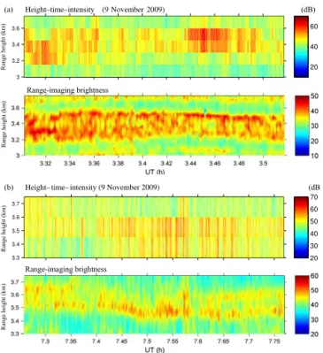
kinds of double thin-layer structures are inspected. In the lower panel of Fig. 8a, a stable double thin-layer structure separated by about 0.2 km was observed in the range inter-val between 3.2 and 3.6 km, which cannot be resolved by the original HTI shown in the upper panel of Fig. 8a. The phys-ical processes involved in the generation of the double thin-layer structure are KHI or vertically propagating wave break-ing, both of which are associated with strong wind shear oc-curring in a very narrow range extent. Strong turbulence mix-ing is expected to occur in the double-layer structure due to dynamic instability, which leads to an enhancement of per-turbation of the atmospheric refractivity and causes intermit-tent occurrences of the relatively intense echoes between the two layers. The lower panel of Fig. 8b presents another type of double thin-layer structure that is characterized by tem-poral merging and separation of the upper and lower thin layers, and exhibits much finer height–time structures than the original HTI shown in the upper panel of Fig. 8b. Notice that, possibly being subject to a broad beam width (∼7.4◦) of
2354 J.-S. Chen et al.: Evaluation of multifrequency range imaging technique
3.32 3.34 3.36 3.38 3.4 3.42 3.44 3.46 3.48 3.5 3
3.2 3.4 3.6
UT (h)
Range (km)
20 40 60
7.3 7.35 7.4 7.45 7.5 7.55 7.6 7.65 7.7 7.75 3.3
3.4 3.5 3.6 3.7
UT (h)
Range (km)
20 30 40 50 60 70
(a) Height–time–intensity (9 November 2009) (dB)
Range-imaging brightness
(b) Height– time– intensity (9 November 2009) (dB)
Range-imaging brightness
Figure 7: Two types of double-layer structures observed on 9 November 2009. In (a, b) both, the upper and lower panels show, respectively, height-time intensity and RIM-produced brightness.
Range
height
(k
m
)
Range
height
(k
m
)
Range
height
(k
m
)
Range
height
(k
m
)
Figure 8. Two types of double-layer structures observed on 9
November 2009. In(a, b)both the upper and lower panels show, respectively, height–time–intensity and RIM-produced brightness.
the billow structures associated with the KHI were difficult to identify.
5 Conclusions
The Chung–Li VHF radar initiated multifrequency experi-ment in 2008, giving the capability of range imaging for detecting finer atmospheric structures in the radar volume. Plenty of radar data have been collected since then, using different radar parameters such as pulse length, pulse shape, receiver bandwidth, transmitter frequency set, and so on. With these radar data, the RIM technique has been evalu-ated widely. Various kinds of thin-layer structures with thick-ness of tens of meters were resolved even though the broad beamwidth of the radar beam may smear the echoing struc-tures. For example, double thin-layer structures having oc-currences of intense echoes within the two layers have been resolved for the first time for the Chung–Li VHF radar.
With the calibration process of RIM conducted in this study, it is found that the typical range/time delay of the sig-nals can be obtained with only two-frequency data as long as the frequency separation of the two frequencies is small. For deriving the optimal range-weighting function, however, the use of seven carrier frequencies with 0.125 MHz frequency step resulted in much more accurate outcomes than the use of two carrier frequencies. A remarkable finding is that the longer the operating hours of the radar system is, the larger the range/time delay will be; this feature is presumably
at-tributed to the aging of cable lines or components in the radar system. One more important finding in this study is a visible shift of range delay when precipitation echoes are signifi-cant, which causes the problem of discontinuity in the RIM-produced brightness at range gate boundaries. We propose in this article a process of point-by-point correction of range error to mitigate the brightness discontinuity to improve the imaging quality of the RIM-produced structures for precipi-tation environment.
Based on the capability of the RIM technique in resolving finer atmospheric structures, it is expected that RIM can help us to reveal more detailed information on the topics of special atmospheric phenomena, such as a tremendously thin layer structure, minute turbulence configuration, and spatial pre-cipitation distribution in the radar volume. It is also expected that in the future the RIM technique in combination with fur-ther modern methods can be applied to the ionosphere for observing plasma density fluctuations in the meteor trail as well as field-aligned plasma irregularities. High resolution at several meters may reveal the delicate structure of plasma irregularities in more detail, which can hopefully help us to understand the temporal evolution of plasma instability at the very beginning stage.
Acknowledgements. This work was supported by the Ministry of
Science and Technology of ROC (Taiwan), grants MOST103-2111-M-039-001 and MOST104-2111-MOST103-2111-M-039-001. The Chung–Li VHF radar is maintained by the Institute of Space Science, National Central University, Taiwan.
Edited by: M. Rapp
References
Chen, J.-S. and Zecha, M.: Multiple-frequency range imaging using the OSWIN VHF radar: phase calibration and first results, Radio Sci., 44, RS1010, doi:10.1029/2008RS003916, 2009.
Chen, J.-S., Su, C.-L., Chu, Y.-H., Hassenpflug, G., and Zecha, M.: Extended application of a novel phase calibration method of multiple-frequency range imaging to the Chung–Li and MU VHF radars, J. Atmos. Ocean. Tech., 26, 2488–2500, 2009. Chen, J.-S., Furumoto, J., and Yamamoto, M.: Three-dimensional
radar imaging of atmospheric layer and turbulence structures us-ing multiple receivers and multiple frequencies, Ann. Geophys., 32, 899–909, doi:10.5194/angeo-32-899-2014, 2014a.
Chen, J.-S., Su, C.-L., Chu, Y.-H., and Furumoto, J.: Measurement of range-weighting function for range imaging of VHF atmo-spheric radars using range oversampling, J. Atmos. Ocean. Tech., 31, 47–61, 2014b.
Chilson, P. B., Yu, T.-Y., Strauch, R. G., Muschinski, A., and Palmer, R. D.: Implementation and validation of range imaging on a UHF radar wind profiler, J. Atmos. Ocean. Tech., 20, 987– 996, 2003.
Chu, Y.-H., Yang, K-.F., Wang, C.-Y., and Su, C.-L: Merid-ional electric fields in layer-type and clump-type plasma struc-tures in mid-latitude sporadic E region: observations and plau-sible mechanisms, J. Geophys. Res.-Space, 118, 1243–1254, doi:10.1002/jgra.50191, 2013.
Fernandez, J. R., Palmer, R. D., Chilson, P. B., Häggström, I., and Rietveld, M. T.: Range imaging observations of PMSE using the EISCAT VHF radar: Phase calibration and first results, Ann. Geophys., 23, 207–220, doi:10.5194/angeo-23-207-2005, 2005. Franke, S. J.: Pulse compression and frequency domain
interferom-etry with a frequency-hopped MST radar, Radio Sci., 25, 565– 574, 1990.
Garbanzo-Salas, M. and Hocking, W. K.: Spectral Analysis com-parisons of Fourier-Theory-based methods and Minimum Vari-ance (Capon) methods, J. Atmos. Sol.-Terr. Phy., 132, 92–100, doi:10.1016/j.jastp.2015.07.003, 2015.
Hassenpflug, G., Yamamoto, M., Luce, H., and Fukao, S.: De-scription and demonstration of the new Middle and Upper at-mosphere Radar imaging system: 1-D, 2-D and 3-D imag-ing of troposphere and stratosphere, Radio Sci., 43, RS2013, doi:10.1029/2006RS003603, 2008.
Hocking, W. K., Hocking, A., Hocking, D. G., and Garbanzo-Salas, M.: Windprofiler optimization using digital deconvo-lution procedures, J. Atmos. Sol.-Terr. Phy., 118, 45–54, doi:10.1016/j.jastp.2013.08.025, 2014.
Lee, C. F., Vaughan, G., and Hooper, D. A.: Evaluation of wind profiles from the NERC MST radar, Aberystwyth, UK, At-mos. Meas. Tech., 7, 3113–3126, doi:10.5194/amt-7-3113-2014, 2014.
Li, J. and Stoica, P.: An adaptive filtering approach to spectral es-timation and SAR imaging, IEEE T. Signal Proces., 44, 1469– 1484, doi:10.1109/78.506612, 1996.
Luce, H., Yamamoto, M., Fukao, S., Hélal, D., and Crochet, M.: A frequency radar interferometric imaging (FII) technique based on high-resolution methods, J. Atmos. Sol.-Terr. Phy., 63, 221–234, 2001.
Luce, H., Hassenpflug, G., Yamamoto, M., and Fukao, S.: High-resolution vertical imaging of the troposphere and lower strato-sphere using the new MU radar system, Ann. Geophys., 24, 791– 805, doi:10.5194/angeo-24-791-2006, 2006.
Luce, H., Hassenpflug, G., Yamamoto, M., Fukao, S., and Sato, K.: High-resolution observations with MU radar of a KH instability triggered 5 by an inertia-gravity wave in the upper part of a jet stream, J. Atmos. Sci., 65, 1711–1718, 2008.
Palmer, R. D., Yu, T.-Y., and Chilson, P. B.: Range imag-ing usimag-ing frequency diversity, Radio Sci., 34, 1485–1496, doi:10.1029/1999RS900089, 1999.
Palmer, R. D., Cheong, B. L., Hoffman, M. W., Fraser, S. J., and López-Dekker, F. J.: Observations of the small-scale variability of precipitation using an imaging radar, J. Atmos. Ocean. Tech., 22, 1122–1137, doi:10.1175/JTECH1775.1, 2005.
Su, C.-L., Chen, H.-C., Chu, Y.-H., Chung, M.-Z., Kuong, R.-M., Lin, T.-H., Tzeng, K.-J., Wang, C.-Y., Wu, K.-H., and
Yang, K.-F.: Meteor radar wind over Chung-Li (24.9◦N,
121◦E), Taiwan, for the period 10–25 November 2012 which includes Leonid meteor shower: Comparison with empirical model and satellite measurements, Radio Sci., 49, 597–615, doi:10.1002/2013RS005273, 2014.
Yamamoto, M. K., Fujita, T., Aziz, N. H. B. A., Gan, T., Hashiguchi, H., Yu, T.-Y., and Yamamoto, M.: Development of a digital re-ceiver for range imaging atmospheric radar, J. Atmos. Sol.-Terr. Phy., 118, 35–44, 2014.
Yu, T.-Y. and Brown, W. O. J.: High-resolution atmospheric pro-filing using combined spaced antenna and range imaging tech-niques, Radio Sci., 39, RS1011, doi:10.1029/2003RS002907, 2004.
Yu, T.-Y. and Palmer, R. D.: Atmospheric radar imaging using spa-tial and frequency diversity, Radio Sci., 36, 1493–1504, 2001. Yu, T.-Y., Furumoto, J., and Yamamoto, M.: Clutter