VALIDATION OF THE DEARDORFF MODEL FOR
ESTIMATING ENERGY BALANCE COMPONENTS FOR A
SUGARCANE CROP
Glauco de Souza Rolim1*; João Francisco Escobedo1; Amauri Pereira Oliveira2
1
UNESP/FCA - Depto. de Irrigação e Drenagem, C.P. 237 - 18610-307 - Botucatu, SP - Brasil. 2
USP/IAG - Depto. de Ciências Atmosféricas, C.P. 66318 - 05508-900 - São Paulo, SP - Brasil. *Corresponding author <[email protected]>
ABSTRACT: The quantification of the available energy in the environment is important because it determines photosynthesis, evapotranspiration and, therefore, the final yield of crops. Instruments for measuring the energy balance are costly and indirect estimation alternatives are desirable. This study assessed the Deardorff’s model performance during a cycle of a sugarcane crop in Piracicaba, State of São Paulo, Brazil, in comparison to the aerodynamic method. This mechanistic model simulates the energy fluxes (sensible, latent heat and net radiation) at three levels (atmosphere, canopy and soil) using only air temperature, relative humidity and wind speed measured at a reference level above the canopy, crop leaf area index, and some pre-calibrated parameters (canopy albedo, soil emissivity, atmospheric transmissivity and hydrological characteristics of the soil). The analysis was made for different time scales, insolation conditions and seasons (spring, summer and autumn). Analyzing all data of 15 minute intervals, the model presented good performance for net radiation simulation in different insolations and seasons. The latent heat flux in the atmosphere and the sensible heat flux in the atmosphere did not present differences in comparison to data from the aerodynamic method during the autumn. The sensible heat flux in the soil was poorly simulated by the model due to the poor performance of the soil water balance method. The Deardorff’s model improved in general the flux simulations in comparison to the aerodynamic method when more insolation was available in the environment.
Key words:energy budget, net radiation, latent heat flux, sensible heat flux, microclimate
VALIDAÇÃO DO MODELO DE DEARDORFF PARA CÁLCULO
DO BALANÇO DE ENERGIA DURANTE UM CICLO DE
CANA-DE-AÇÚCAR
RESUMO: A quantificação da energia disponível no ambiente é importante porque ela afeta a fotossíntese, a evapotranspiração e conseqüentemente a produtividade final dos cultivos. Instrumentos para medidas de balanço de energia são caros e alternativas para estimações são desejáveis. O presente trabalho procura avaliar a performance do modelo de Deardorff (1978) ao longo do desenvolvimento de uma cultura de cana-de-açúcar em Piracicaba, SP, Brasil, em comparação ao método aerodinâmico. Este modelo mecanístico simula os fluxos energéticos (calor sensível, latente e saldo de radiação) em três níveis: a atmosfera, o dossel vegetativo e o solo, usando somente a temperatura do ar, umidade relativa e velocidade do vento medidos num nível de referência acima do dossel, o índice de área foliar e alguns parâmetros previamente calibrados (albedo do dossel, emissividade do solo e a transmissividade atmosférica e características hidrológicas do solo). As análises dos resultados foram feitas em diversas escalas de tempo, condições de insolação, nas diferentes estações do ano (primavera, verão, outono). Analisando todos os dados de 15 minutos, o modelo apresentou boa performance na simulação de radiação líquida em diferentes condições de insolação e estações do ano. O fluxo de calor latente e o fluxo de calor sensível na atmosfera não apresentaram diferenças em comparação ao método aerodinâmico no outono. O calor sensível no solo foi pobremente simulado pelo modelo devido à baixa capacidade de estimação do balanço hídrico do solo. Geralmente as estimações pelo modelo de Deardorff foram melhoradas quando mais insolação era disponível no ambiente.
INTRODUCTION
Studies on energy balance of agricultural ar-eas allow the understanding of energy change pro-cesses in relation to evapotranspiration and photosyn-thesis, which directly affect the biomass accumulation and agricultural yield. Several studies can be cited, as those related to evapotranspiration estimations (Villa Nova et al., 2007), to leaf wetness duration and its consequences on pathogen infection processes (Marta et al., 2007), and to the development of mechanistic crop growth models (Pauwels et al., 2007), among oth-ers.
Several methods are available to estimate the energy balance of the environment, also when there is data limitation. The models presented by Shuttleworth & Wallace (1985), Zapata & Martinez-Cob (2002) and Hemakumara et al. (2003) are ex-amples of them. At the mesoclimatic scale, the Deardorff’s (1978) model has been used with suc-cess to simulate energy fluxes (Soares et al., 1996; Targino & Soares, 2002). Vogel et al. (1995) ob-served that Deardorff’s (1978) model presented a better performance simulating the sensible heat flux (in air and soil) than other models, when applied to vegetated surfaces.
At the microclimatic scale, few agricultural studies can be found using the Deardorff (1978) model. Tattari et al. (1995) tested Deardorff’s (1978) model and compared it to the Bowen’s ratio method to estimate barley crop evapotranspiration, but the re-sults were not very good due to problems with mea-surements made under adverse climatic conditions, such as high humidity, gusts of wind and rain. How-ever, McCumber (1980) and Garret (1982) stated that among the methods found in the literature, the one pro-posed by Deardorff (1978) is the most efficient to esti-mate energy balances with quality and simplicity. Fi-nally, Oliveira et al. (1999) working with maize and grass crops at Candiota, RS, Brazil, obtained good re-sults in simulations of sensible and latent flux and net radiation.
The advantage of using the model proposed by Deardorff (1978) is the significant reduction of the number of instruments required to estimate the energy balance of a given crop, since it only re-quires air temperature, relative humidity, wind speed, leaf area index and some hydrological parameters of the soil. This study analyses the performance of Deardorff’s (1978) model to estimate net radia-tion, latent heat flux, sensible heat flux in the atmo-sphere and in the soil, during a complete cycle of a sugarcane crop, in comparison to the aerodynamic method.
MATERIAL AND METHODS
Site descriptions and measurements
The sugarcane cultivar IAC 87-3396 used in this study was sown on 12/08/2001 with 1 meter row spacing in the east-west orientation. The experimental field is characterized by a flat area of about 1 km2,
located in Piracicaba, Sate of São Paulo, Brazil (22º40’ S, 47º38’ W and altitude 514 m). The meteorological data, were collected each second and integrated ev-ery 15 seconds, from 08/17/2001 to 05/31/2002 us-ing a Campbell 21X datalogger and sensors previously calibrated. The sensors were mounted on a tower at the center of the area and the measurements were made at six levels: 5 m from the surface (rain); 2 m from the top of the canopy (temperature, relative humidity, wind speed, net radiation, global and reflected solar radiation); ¾ of canopy height (temperature, relative humidity and wind speed); on the soil surface (heat flux); in the soil, 5 and 20 cm below the surface (tem-perature and humidity). The levels: 2 m from the top of the canopy and ¾ of canopy height were adjusted monthly to follow crop growth. The 2 m level men-tioned above, contains the necessary data for Deardorff’s (1978) model inputs (temperature, relative humidity and wind speed) and the extra observations were necessary for model comparisons.
The sugarcane crop was chosen due to its great economic interest in State of São Paulo, besides its long cycle which makes possible performance analyses of the model during several seasons of the year.
Determination of the energy balance components by the aerodynamic method
The estimation of the energy balance compo-nents (Rn – Net radiation, LE – Latent heat flux, H – sensible heat flux in the atmosphere and G- Sensible heat flux in the soil) by the aerodynamic method us-ing data observed in the field was made to compare the simulated data obtained by the Deardorff's (1978) model.
From data obtained every 15 seconds the Richardson number (Ri) was calculated in order to compare the thermal forces responsible for the free convection, with the mechanical forces responsible for the forced convection. The Richardson number was calculated by the following equation:
2 ) / .(
/ .
dz du m
dz d g Ri
Θ Θ
= (1)
tem-perature is calculated by Q = air temperature
(K).(1000/800)0.2857.
In order to estimate the effect of Ri on the tur-bulent diffusion coefficient (Km), which makes pos-sible to quantify the transport of atmospheric activity (sensible and latent heat flux) the function φm was cal-culated for the following cases: unstable conditions (when Ri < 0): φm = (1–16.Ri)-0.25; stable conditions
(when Ri > 0): φm = 1 + 5.Ri; and neutral conditions (when Ri = 0): φm= 1
The turbulent diffusion coefficient (Km) is given by:
2 2 2
. . ) .(
m dz
du d
z k Km
φ
−
= (2)
where: k is the von Karman constant (= 0.41), z the reference sensor height and d is the zero place dis-placement (considered ¾ of the canopy height). The coefficient Km was used to estimate the sensible heat flux:
dz dT Km Cp
H =−ρ. . . (3)
where: ρ is air density (=1,292 kg m-3), Cp the
spe-cific heat of dry air at constant pressure (= 1,005 kJ kg-1 K-1) and dT/dz the temperature gradient between
the two sensors.
The values of the sensible heat flux in the soil (G) and net radiation (Rn) were obtained directly from field measurements and when H was possible to be calculated, the latent heat flux value (LE) was obtained from:
LE = Rn – H – G (4)
Deardorff’s (1978) model
The Deardorff’s (1978) model comprises sev-eral stages, however some relevant aspects can be briefly described: the model considers that there is only one vegetation layer, whose thermal capacity is insig-nificant and characterized by a coefficient (σf) that is
associated with the degree to which the canopy pre-vents the shortwave radiation to reach the soil, which is calculated using the leaf area index (LAI). σf = 0
refers to absent vegetation cover and σf = 1 to
com-plete vegetation cover (theoretical).
With the coefficient σf and considering the
wind logarithmic profile, three heat transfer coeffi-cients can be calculated for the following levels: bare soil surface (CH0 = k2.ln(z/z
o)-2, where k = 0.4; z = 2
m above the canopy and zo = roughness parameter);
high immediately above the canopy top (CHh = (1/ k).ln[(z-d)/zoh]), where d = zero plane displacement
= ¾. Canopy high; zoh = (canopy high – d)/3); soil
surface (CHg = (1-σf).CH0 + σf.CHh ).
Using the coefficient CHh at the reference level
(ua), the mean speed inside the canopy (uaf) is
calcu-lated by:
uaf = 0.38s f cHh
1/2
ua + (1 – s f) ua (m s
-1) (5)
where: ua is the wind speed (m s-1) measured at
refer-ence level
It was assumed that the inner part of the canopy presents average conditions between the atmo-sphere and the soil, thus the air temperature inside the vegetation (Taf) and the correspondent humidity (qaf)
were calculated by the following equations:
Taf = (1 –σf) Ta + σf (0.3Ta + 0.6Tf + 0.1Tg) (ºC) (6)
qaf = (1 – sf) qa + σf (0.3qa + 0.6qf + 0.1qg) (cm
3 cm-3)
(7)
where: Tf = average leaf temperature, Tg = soil sur-face temperature, Ta = temperature at the reference level (measured) and qaf , qg , qa and qf are analogous
specific humidities.
In a simple way, Tf, and qf have been estimated from the energy balance at the level of a single leaf inside the canopy. This is an iterative calculation pro-cedure that aims to minimize the differences in the fol-lowing equation:
) ( Sg Lg Sg Lg
Lh Sh Lh
Sh R R R R R R R
R↓ + ↓ − ↑ − ↑ − ↓ + ↓ − ↑ − ↑ =
) ( h g
sg
sh H E E
H − + −
= λ (8)
where: RS, RL, Hs and E are short and long wave ra-diative fluxes, sensible heat flux and evapotranspira-tion, respectively, and l is the evaporation latent heat. The subscribed letters h and g represent values at the canopy top and on the soil surface, respectively. Fi-nally, the arrows indicate the radiative flux directions. When the Stefan-Boltzmann’s equation is used in each side of the equation 8 and other changes mentioned by Deardorff (1978) are introduced, the result is equa-tion 9, which must be solved to find the representa-tive canopy leaf temperature:
g g f g f
g f Lh
f Sh f
f R R ε ε ε ε σT
ε ε ε
α
σ −
− + + +
− ↓ ↓
) (
) 1
[( 4
f f f f g f g f
g f g f
E Hs
T λ
σ ε ε ε ε ε
ε ε ε ε
+ = −
+ − +
− ]
) (
) 2
( 4
(9)
where: αf and εf are the albedo and the foliage
emis-sivity, εg is the soil emissivity and s is the
Stefan--Boltzmann constant (5.67 × 10⁻⁸ W m-2 K-4).
the energy flux sum in the atmosphere and contains a mechanism that causes an influence of the deep soil layers on the surface temperature. Thus, the soil is di-vided in two layers: a superficial one, for which the soil temperature is influenced by the daytime cycle, and a deep one, of infinite depth in which the temperature changes in an annual scale, as follows:
1 2 1
1 2
τ ρ
T Tg c d c H c t T
s s
A
g =− − −
∂ ∂
(10)
where: T2 is the average temperature of the soil in the deep layer; c1 and c2 are dimensionless constants; ρs
is the soil density; cs the soil specific heat; d1 the soil depth under the influence of daytime cycle; and τ1 is
the photoperiod; HA is the sum of the atmospheric fluxes at the surface as a result of the energy balance at the soil surface.
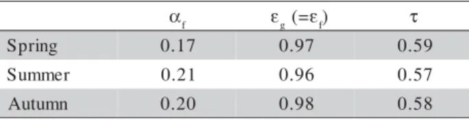
Finally, the Deardorff’s (1978) model, besides temperature, relative humidity and wind speed data, requires some parameters that were previously cali-brated (Table 1). Basically, the calibration of these pa-rameters aimed to an approach between the measured and simulated data by the model, using the iterative method Simplex with initial values of εf = 0.95; εg =
0.95; αf = 0.2 according to results of Targino & Soares
(2002) and τ = 0.7. A total of 12 days were used for this process (4 days of each season with different in-solation conditions), considering the available 249 days. These parameters are similar to those found in literature, as Monteith & Unsworth (1990), who re-lated an emissivity for a sugarcane surface of 97.7 ± 0.4%. Gates (1980), on the other hand, found an al-bedo of 0.17 during the complete development of a given sugarcane crop. Finally, Unsworth & Monteith (1972), who made atmospheric transmissivity measure-ments in England, obtained values of 0.95 for very clear days and 0.5 for days with too much pollution or for cloudy sky conditions.
The Deardorff’s (1978) model also requires three soil hydrologic parameters: water contents at wiltting point (wwilt), at field capacity (Wk) and at satu-ration (Wmax). In relation to this a physico-hydric analysis of the soil was accomplished giving empha-sis on the determination of the soil water
characteris-tic curve. The results were: wwilt = 0.15; Wk = 0.21;
Wmax = 0.32 (cm3 cm-3).
Biometrical measurements of the sugarcane crop The parameters that affect the logarithmic wind profile above canopy, leaf area (LA) and aver-age height of the canopy, were measured every 15 days from 08/17/2001 to 05/30/2002, considering five rep-lications. The leaf area index (LAI) was determined by collecting and measuring leaves from a randomized area of 1 m2, using a paper guide with accuracy of 1 mm.
Evaluation of Deardorff’s (1978) model
The data simulated by the model (SIM): Taf, uaf, canopy relative humidity (RHcanopy), Rn, LE, H, G,
were compared to those calculated by the aerodynamic method (AERO) using the index of agreement id sug-gested by Willmott (1981):
(
21 1
2
) ( 1
å
å
= =
-+
-=
N
i
i i
N
i
i i
d
O O O P
O P
i
(
(11)where: id is dimensionless and ranges from 0 (zero)
to 1, considering that the value 1 indicates complete agreement between observed and estimated values; Pi are SIM values; Oiare AEROvalues; the mean of AERO values and N the number of observations.
RESULTS AND DISCUSSION
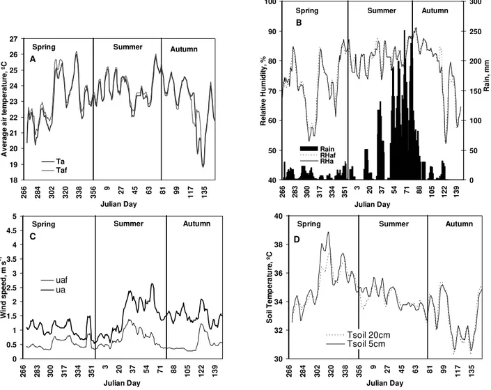
Meteorological elements inside the canopy were directly affected by crop development. The in-crease of the leaf area index and canopy height (Fig-ure 3) affected the wind speed inside the canopy (uaf), which was reduced in relation to the reference level (Figure 1C). Because of that, the difference uref - ua was smaller during the spring than in the autumn. Fig-ure 1D shows that soil temperatFig-ure (5 and 20 cm) was reduced during the crop growth.
The five-day moving average of Rn ranged from 500 W m-2 to 700 W m-2 from summer to spring
and from 450 W m-2 to 600 W m-2 during autumn
(Fig-ure 2). The first summer weeks presented maximum values of LE, up to 490 W m-2, whereas in middle of
autumn they reached only 150 W m-2.
The maximum LAI and height found for sug-arcane crop were 4.6 and 2.8 m, respectively (Figure 3). These results also correspond to those found in the literature, e.g. Leme et al. (1984), who observed a maximum LAI of 4.5 for the sugarcane cultivar CB47-355, and Bull & Glasziou (1975) and Machado et al. (1982) that also observed that the crop reached a maximum height of 2.6 m.
αf εg(=εf) τ
g n i r p
S 0.17 0.97 0.59
r e m m u
S 0.21 0.96 0.57
n m u t u
A 0.20 0.98 0.58
Table 1 - Calibrated dimensionless parameters used in the Deardorff’s (1978) model: αf - canopy albedo, εg
- soil emissivity, εf canopy emissivity, and t -atmospheric transmissivity.
Figure 1 - Five-day moving averages of measured meteorological variables inside the canopy (3/4 of canopy height) and at the reference level (2 meters above canopy): A) Temperature, B) Relative humidity and accumulated rain, C) Wind speed, D) Soil temperature (5 and 20cm below the surface).
18 19 20 21 22 23 24 25 26 27
26
6
28
4
30
2
32
0
33
8
35
6 9
27 45 63 81 99
11
7
13
5
Julian Day
A
v
erag
e a
ir t
e
m
p
erat
u
re, º
C
Ta Taf
Spring Summer Autumn
A
40 50 60 70 80 90 100
266 283 300 317 334 351
3
20 37 54 71 88 105 122 139
Julian Day
Re
la
ti
v
e
Hu
m
id
it
y
, %
0 50 100 150 200 250 300
R
a
in
, m
m
Rain RHaf RHa
Spring Summer Autumn
B
0 0.5 1 1.5 2 2.5 3 3.5 4 4.5 5
26
6
28
3
30
0
31
7
33
4
35
1 3
20 37 54 71 88
10
5
12
2
13
9
Julian Day
W
in
d
sp
ee
d
, m
s
-1
uaf ua
Spring Summer Autumn
C
30 32 34 36 38 40
26
6
28
4
30
2
32
0
33
8
35
6 9
27 45 63 81 99
11
7
13
5
Julian Day
S
o
il T
e
m
p
era
tu
re,
º
C
Tsoil 20cm Tsoil 5cm
Spring Summer Autumn
D
Figure 2 - Five-day moving average of maximum hourly values of energy balance components (Rn – Net radiation, LE – Latent heat flux, H – Sensible heat flux at the atmosphere and G – Sensible heat flux in the soil) estimated by the aerodynamic method.
0 100 200 300 400 500 600 700 800
26
6
27
9
29
2
30
5
31
8
33
1
34
4
35
7 5
18 31 44 57 70 83 96 109 122 135 148
Julian Day
E
n
er
g
et
ic f
lu
x
, W
m
-2
Rn LE H (-)G
Spring Summer Autumn
The best meteorological variable simulated by the Deardorff (1978) model was the air temperature inside the canopy (Taf). The smallest errors for all sea-sons were found next to midday. At other periods, the
model had a tendency to underestimation, however, mean absolute differences of no more than 3oC were
found.
As expected, the minimum hourly tempera-ture inside the canopy always occurred between 6h00 and 7h00 a.m., with values around 16ºC during spring and autumn, and around 18ºC during summer, while the mean temperature inside the canopy remained around 27ºC in spring, 30ºC in summer and 28ºC in autumn.
Deardorff’s (1978) model also presented a good performance for simulating temperature at the canopy level (Taf) in days with different insolation
con-ditions. The id index was always higher than 0.83, de-spite of some variability noticed by R2 values around
0.49, or moreover, by the coefficient of variation (CVSIM), around 22% (Table 2).
Figure 3 - A) Leaf area index variation (LAI); B) canopy height variation of the variety IAC 87-3396 of sugarcane between August 17, 2001 and May 30, 2002.
0 1 2 3 4 5
229 245 263 281 299 317 334 352
5
23 41 59
Julian day
L
e
af
A
rea
I
n
d
e
x
(
m
2 m -2 )
Adjusted Observed
A
0 1 2 3
229 245 263 281 299 317 334 352
5
23 41 59
Julian day
C
a
no
py
h
e
igh
t
(m
)
B
for vegetated surfaces was efficient to represent field conditions. The simulated uaf did not differ from the observed uaf, despite to the low values of R2 (Table 2),
since the greatest daily mean differences found were of 0.57 m s-1 in summer, 0.51 m s -1 in autumn and a
little higher in spring, reaching 0.78 m s-1. The small
values of R2 and high values of i
d, indicated that the
model did not follow instantaneous variations of the wind speed but the magnitude of adjustments in subsequent moments was good. The relationships between AERO and SIM data were less significant in spring, when the sugarcane crop was in the first stages of development. Still considering the canopy level, the last me-teorological variable analyzed was the canopy relative humidity (RHcanopy). The SIM values were not close to those found by AERO due the low values of R2,
de-spite of the high values of id, and mainly, because the obtained mean differences were of 8.96%, 12.04% and 6.5% in the spring, summer and autumn, respectively.
For all seasons there was a high variability of AERO for 15 minute averages of relative humidity, re-sulting in small R2 values when compared with SIM.
The model presented a tendency of underestimation
under high relative humidity, mostly before sunrise, and a tendency of overestimation under low relative hu-midity, close to 2h00 p.m.
Finally, when SIM and AERO are compared for all meteorological variables when extra insolation was available in the environment, there was an increase of id and R2 (Table 2).
In summary, high values of id indicate that SIM values are close to AERO, that is, close to the 1:1 line. On the other hand, the small values of R2 indicate that
SIM and AERO data often have a high dispersion. The simulations of soil water content were worse than those at the canopy level, which is related to the low ca-pacity of the Deardorff (1978) model in simulating the soil water balance for successive days, as shown in Figure 4A.
The model was not able to simulate the dry-ing of the soil (Figure 4), even though after long drought periods like at the end of spring and autumn, yielding different values from the AERO soil moisture. Thus, 57% of the days in spring and summer and 86% of the days in autumn, the simulated soil moisture in the root zone was above the observed values.
Figure 4 - Daily mean soil moisture (A) and soil thermal diffusivity (ks) (B) simulated by Deardorff’s (1978) model (SIM) and calculated by the aerodynamic method (AERO) during spring, summer and autumn seasons.
0 0.05 0.1 0.15 0.2 0.25 0.3 0.35 0.4
266 282 298 314 330 346 362 14 30 46 62 78 94 110 126 142
Julian day SIM Soil moisture OBS Soil moisture
Spring Summer Autumn A
wa
te
r c
o
n
te
n
t (m
3 m -3 )
0 0.002 0.004 0.006 0.008 0.01 0.012 0.014
266 282 298 314 330 346 362 14 30 46 62 78 94 110 126 142
Julian day
S
o
il
t
h
e
rm
a
l d
if
fu
s
iv
it
y
K
s
(
c
m
2 s -1 )
Ks SIM Ks OBS
Deardorff model for estimating energy balance
331
.65, n.4, p.325-334, July/August 2008
Deardorff’s (1978) model (SIM) and calculated by the aerodynamic method (AERO) inside the canopy: air temperature (Taf, ºC), relative humidity (RH, %) and wind speed (uaf, m s-1) for different seasons of the year and different insolation levels.
n o s a e S
n o i t a l o s n I
) r u o h (
º n
s y a d
) C º ( f a T , e r u t a r e p m e t r i a y p o n a
C Canopywind speed, uaf(ms-1) RelativeHumidity,RH
y p o n a
c (%)
id R2 Averg.
M I S
. g r e v A
O R E A
D S
M I S
D S
O R E A
V C
M I S
V C
O R E
A id R2
. g r e v A
M I S
. g r e v A
O R E A
D S
M I S
D S
O R E A
V C
M I S
V C
O R E
A id R2
. g r e v A
M I S
. g r e v A
O R E A
D S
M I S
D S
O R E A
V C
M I S
V C
O R E A
g n i r p
S All 89 0.88 0.68 21.68 23.24 5.24 4.49 0.24 0.19 0.490.13 1.54 0.55 0.93 0.45 0.60 0.83 0.680.28 80.72 71.76 14.9019.62 0.18 0.27
3 < x = <
0 19 0.86 0.65 21.74 23.65 4.75 4.18 0.22 0.18 0.490.08 1.49 0.62 0.95 0.46 0.64 0.74 0.580.16 85.20 73.69 12.4417.09 0.15 0.23
7 < x = <
3 18 0.84 0.58 21.65 23.10 4.19 3.99 0.19 0.17 0.490.16 1.63 0.54 1.00 0.43 0.61 0.80 0.550.16 85.18 75.72 11.0516.97 0.13 0.22
0 1 < x = <
7 26 0.88 0.67 21.35 22.75 5.49 4.87 0.26 0.21 0.48 0.11 1.51 0.48 0.82 0.36 0.55 0.75 0.640.18 77.32 70.47 14.8119.42 0.19 0.28
x = < 0
1 26 0.90 0.77 21.98 23.54 5.93 4.59 0.27 0.20 0.520.18 1.55 0.57 0.95 0.53 0.62 0.94 0.780.46 77.77 68.91 17.1522.47 0.22 0.33
r e m m u
S All 89 0.85 0.58 22.66 23.74 4.61 3.88 0.20 0.16 0.510.07 1.04 0.52 0.75 0.38 0.72 0.73 0.400.03 92.96 80.92 9.06 15.24 0.10 0.19
3 < x = <
0 19 0.87 0.61 22.43 23.51 4.33 3.98 0.19 0.17 0.490.07 1.15 0.53 0.82 0.37 0.72 0.70 0.510.07 90.95 80.07 11.3515.97 0.12 0.20
7 < x = <
3 18 0.83 0.49 22.93 23.71 4.36 3.71 0.19 0.16 0.490.03 1.06 0.56 0.77 0.42 0.73 0.74 0.35 0.01 93.27 81.46 7.96 13.96 0.09 0.17
0 1 < x = <
7 26 0.84 0.57 22.93 23.84 5.05 3.81 0.22 0.16 0.500.07 1.04 0.46 0.71 0.31 0.68 0.67 0.34 0.01 94.39 81.48 7.25 15.10 0.08 0.19
x = < 0
1 26 0.88 0.69 22.31 23.86 4.58 4.04 0.21 0.17 0.560.13 0.94 0.53 0.68 0.40 0.73 0.75 0.400.02 92.84 80.49 9.37 15.96 0.10 0.20
m m u t u
A All 89 0.89 0.70 21.59 22.85 4.90 4.25 0.23 0.19 0.650.25 1.23 0.75 1.13 0.72 0.92 0.96 0.760.36 83.21 76.71 17.5320.57 0.21 0.27
3 < x = <
0 19 0.86 0.71 21.41 23.22 4.51 3.59 0.21 0.15 0.640.21 1.25 0.82 1.08 0.76 0.87 0.92 0.740.39 88.86 80.64 13.9018.60 0.16 0.23
7 < x = <
3 18 0.91 0.75 22.32 23.43 4.34 4.02 0.19 0.17 0.660.28 1.07 0.66 1.12 0.68 1.05 1.02 0.77 0.41 86.33 77.66 16.0920.39 0.19 0.26
0 1 < x = <
7 26 0.90 0.68 21.12 22.08 5.03 4.70 0.24 0.21 0.630.23 1.43 0.81 1.20 0.76 0.84 0.94 0.710.23 78.08 74.81 16.6520.30 0.21 0.27
x = < 0
1 26 0.88 0.72 22.01 23.43 5.15 3.88 0.23 0.17 0.690.31 1.03 0.67 1.01 0.64 0.98 0.69 0.810.50 85.52 76.45 19.6721.92 0.23 0.29
e g a r e v
Soil moisture tends to damp the soil against sud-den changes in temperature, since the heat moves from the soil to the water about 150 times easier than from the soil to the air (Brady, 1989). Therefore, if the simu-lated soil moisture by Deardorff’s (1978) model is higher than expected, the simulated thermal capacity of this soil is also higher than the observed one. Conse-quently, it makes higher temperature variations in the soil more difficult, indicating that the simulated thermal difusivity (Figure 4B) of this soil may be lower as well. This supposition was confirmed by Rolim (2003), with the similar data, because the amplitude of soil tempera-ture variations (on surface and at the 20 cm depth) were actually lower than the observed ones, resulting in low values of id and R2 for all seasons.
Despite these differences found between the observed meteorological elements and those simulated by Deardorff’s model, one can see (Table 3) that simu-lations of the energy balance components – Net Ra-diation (Rn), Latent heat flux (LE) and Sensible heat flux at the atmosphere (H) (Table 4) – do not present distinction in relation to the AERO fluxes during all the seasons of the year and in different insolation levels for the sugarcane crop, except the sensible heat flux in the soil (G).
Differences between Rn from AERO and the SIM data at every 15 minute interval were small, con-sidering the high values of id and R2 for all seasons
(Table 3), with exception to summer (d = 0.79, R2 =
0.50) due to a greater nebulosity and occurrence of rain (Figure 1B), because there was as well a tendency to improve Rn estimates as the insolation availability increased (Table 3).
This similarity between AERO and SIM data of Rn is also due, among other reasons, to the fact that Deardorff’s model made a good approach to the total albedo data of the surface (maximum val-ues: spring = 0.34; summer = 0.36 and autumn = 0.33), that directly affects the amount of radiation available in the system soil-vegetation-atmosphere (Figure 5).
Relationships between the AERO and SIM data at every 15 minute intervals of latent heat flux in the atmosphere (LE) (Table 3) and sensible heat flux in the atmosphere (H) (Table 4) also were high, taking into account the values of id found for all seasons. The
lower values of id during the summer were, on account of the same reasons already discussed in relation to Rn, due to the sensibility of the Deardorf’s (1978) model in relation to the available insolation.
Table 3 - Determination Coefficient (R2), Willmott Coefficient (i
d), average, standart deviation (SD) and Coefficient of Variation (CV) of 15 minute data simulated by Deardorff’s (1978) model (SIM) and calculated by the aerodynamic method (AERO) of Net Radiation (Rn, W m-2) and Latent Heat Flux (LE, W m-2) in different seasons of the year and for different insolation levels.
n o s a e
S Insolation ) r u o h
( nº s y a d
m W ( n R , n o i t a i d a R t e
N -2) Latentheatflux, LE(Wm-2)
id R2 Averg. M I S
. g r e v A
O R E A
D S
M I S
D S
O R E A
V C
M I S
V C
O R E
A id R2
. g r e v A
M I S
. g r e v A
O R E A
D S
M I S
D S
O R E A
V C
M I S
V C
O R E A g
n i r p
S All 89 0.870.66185.54107.19260.14 214.54 1.40 2.00 0.690.50155.00 59.65217.39103.211.40 1.73 3
< x = <
0 19 0.880.68174.94104.93247.77 205.89 1.41 1.96 0.710.49134.22 58.39 199.8199.69 1.48 1.70 7
< x = <
3 18 0.810.54179.5288.97251.05 189.98 1.39 2.13 0.650.46154.73 50.44214.5591.26 1.38 1.80 0
1 < x = <
7 26 0.880.67188.00113.88263.12 225.83 1.39 1.98 0.700.52160.00 62.36223.40108.281.39 1.73 x
= < 0
1 26 0.880.70194.99114.76271.66 224.29 1.39 1.95 0.690.50165.38 64.24224.57107.861.35 1.67 r
e m m u
S All 89 0.790.49185.5388.97252.37 187.31 1.36 2.10 0.660.88143.16 54.31212.23102.721.48 1.89 3
< x = <
0 19 0.810.52181.6496.07248.82 195.94 1.36 2.03 0.680.39133.40 57.13199.89103.431.49 1.81 7
< x = <
3 18 0.760.45189.3179.42 252.66 175.29 1.33 2.20 0.620.27137.0147.99204.5296.05 1.49 2.00 0
1 < x = <
7 26 0.790.50192.8190.67259.68 187.00 1.34 2.06 0.660.40158.42 55.94229.30104.551.44 1.86 x
= < 0
1 26 0.800.51177.3890.86247.10 191.69 1.39 2.10 0.670.37141.45 56.62210.46106.401.48 1.87 m
m u t u
A All 89 0.940.82125.8094.81 211.90 188.10 1.68 1.98 0.930.98 94.38 54.54157.7394.04 1.67 1.72 3
< x = <
0 19 0.940.81132.67100.89215.40 193.88 1.62 1.92 0.770.54 94.67 55.78 158.7195.06 1.67 1.70 7
< x = <
3 18 0.940.83129.3598.98213.07 185.32 1.64 1.87 0.810.64 91.12 57.40154.6393.30 1.69 1.62 0
1 < x = <
7 26 0.920.76124.0790.15212.89 187.99 1.71 2.08 0.800.65 92.34 50.52157.0589.98 1.70 1.78 x
= < 0
1 26 0.970.92121.7295.48207.27 186.02 1.70 1.94 0.850.76 99.37 58.21160.0499.68 1.61 1.71 e
g a r e v
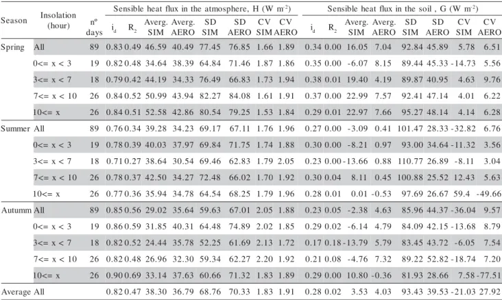
Table 4 - Determination Coefficient (R2), Willmott Coefficient, (i
d), Mean, standart deviation (SD) and Coefficient of Variation (CV) of 15 minute data simulated by Deardorff’s (1978) model (SIM) and calculated by the aerodynamic method (AERO) for the Sensible Heat Flux (H, W m-2) in the atmosphere, Sensible Heat Flux (H, W m2) in the soil (G, W m-2) for different seasons of the year and at different insolation levels.
n o s a e
S Insolation ) r u o h
( nº s y a d m W ( H , e r e h p s o m t a e h t n i x u l f t a e h e l b i s n e
S -2) Sensibleheatfluxinthesoil,G(Wm-2)
id R2 Averg. M I S . g r e v A O R E A D S M I S D S O R E A V C M I S V C O R E
A id R2
. g r e v A M I S . g r e v A O R E A D S M I S D S O R E A V C M I S V C O R E A g n i r p
S All 89 0.830.49 46.59 40.49 77.45 76.85 1.66 1.89 0.340.00 16.05 7.04 92.84 45.89 5.78 6.51 3
< x = <
0 19 0.820.48 34.64 38.39 64.84 71.46 1.87 1.86 0.350.00 -6.07 8.15 89.44 45.33-14.73 5.56 7
< x = <
3 18 0.790.42 44.19 34.33 76.49 66.83 1.73 1.94 0.380.01 19.40 4.19 89.87 40.95 4.63 9.76 0 1 < x = <
7 26 0.840.52 50.99 43.94 82.27 84.08 1.61 1.91 0.370.00 22.99 7.57 92.41 47.14 4.01 6.22 x
= < 0
1 26 0.840.51 52.58 42.86 80.54 79.25 1.53 1.84 0.290.01 22.97 7.66 95.27 48.14 4.14 6.28 r
e m m u
S All 89 0.760.34 39.28 34.23 69.17 67.11 1.76 1.96 0.270.00 -3.09 0.41 101.47 28.33-32.82 6.76 3
< x = <
0 19 0.780.39 40.03 37.97 69.84 71.75 1.74 1.88 0.300.00 -8.21 0.97 93.00 34.64-11.32 3.56 7
< x = <
3 18 0.710.27 38.64 30.54 69.46 62.83 1.79 2.05 0.230.00-13.66 0.88 110.77 26.89 -8.11 3.04 0 1 < x = <
7 26 0.780.37 42.50 34.27 72.48 66.02 1.70 1.92 0.300.04 8.11 0.45 100.88 25.52 12.43 5.63 x
= < 0
1 26 0.770.36 35.94 34.78 64.54 68.25 1.79 1.96 0.280.01 0.01 -0.53 97.69 26.67 59.4 -49.66 m
m u t u
A All 89 0.850.56 29.02 35.64 59.63 67.01 2.05 1.88 0.230.05 -2.38 4.63 85.96 44.37-36.04 9.57 3
< x = <
0 19 0.860.59 31.85 40.31 64.48 74.89 2.02 1.85 0.290.02 -6.14 4.79 84.09 42.15-13.68 8.79 7
< x = <
3 18 0.820.52 24.44 35.78 52.25 61.69 2.13 1.72 0.170.18-13.79 5.79 83.45 43.72 -6.05 7.54 0 1 < x = <
7 26 0.820.48 26.96 32.30 59.34 62.27 2.20 1.92 0.210.08 -4.76 7.32 89.22 52.82-18.74 7.20 x
= < 0
1 26 0.900.69 33.14 37.63 60.66 71.32 1.83 1.89 0.290.00 10.80 -0.36 81.93 28.66 7.58-77.51 e g a r e v
A All 0.820.47 38.30 36.79 68.76 70.33 1.83 1.91 0.280.02 3.53 4.03 93.43 39.53-21.0327.92
Figure 5- Hourly average albedo simulated by Deardorff (1978) model (SIM) and calculated by aerodynamic method (AERO) during spring (A), summer (B) and autumn (C) seasons.
Finally, there was no agreement between AERO and SIM data of sensible heat fluxes in the soil (G), as verified in different seasons of the year (Table 4). This fact is a consequence of the low variation of the simulated thermal difusivity, which is a result of the low variation of the water contents in the soil profile, or in a broad way, is a result of the low capacity of the Deardorff model in simulating of the crop water budget. Despite the low relationships of G, the model could recalculate the energy balance making the estimatives of Rn, LE and H statistically close. In this way the model becomes interesting for agrometeorological purposes, since it needs only a few measured data at a reference level.
CONCLUSIONS
The latent heat flux and the sensible heat flux at the atmosphere, simulated by Deardorff’s (1978) model did not presented differences in comparison to the aerodynamic method in the autumn of Piracicaba, State of São Paulo, Brazil. The greatest differences between the Deardorff (1978) model and the aerody-namic method were found in the simulations of the sensible heat flux in the soil.
ACKNOWLEDGEMENTS
To FAPESP for financial support and the Instituto Agronômico- IAC, Piracicaba for the experi-mental area.
REFERENCES
BHUMRALKAR, C.M. Numerical experiments on the computation of ground surface temperature in an atmospheric general circulation model. Journal of Applied Meteorology, v.14, p.1246-1258, 1975.
BRADY, N.C. Natureza e propriedades dos solos. Rio de Janeiro: Freitas Bastos, 1989. 878p.
BULL, T.A.; GLASZIOU, K.T. Sugar cane. In: EVANS, L.T. (Ed.) Crop physiology: some case histories. Cambridge: Cambridge University Press, 1975. cap.3, p.51-72.
DEARDORFF, J.W. Efficient prediction of ground surface temperature and moisture, with inclusion of a layer of vegetation. Journal of Geophysical Research, v.83, p.1889-1903, 1978. GARRET, A.J. A parameter study of interactions between convective clouds, the convective boundary layer, and a forested surface. Monthly Weather Review, v.110, p.1041-1059, 1982. GATES, D.M. Biophysical ecology. New York: Springer, 1980.
611p.
HEMAKUMARA, H.M.; CHANDRAPALA, L.; MOENE, A.F. Evapotranspiration fluxes over mixed vegetation areas measured from large aperture scintillometer. Agricultural Water Management, v.58, p.109-122, 2003.
LEME, E.J.A.; MANIEIRO, M.A.; GUIDOLIN, J.C. Estimativa da área foliar da cana-de-açúcar e sua relação com a produtividade.
Cadernos PLANALSUCAR, n.2, p.3-9, 1984.
MACHADO, E.C.; PEREIRA, A.R.; FAHL, J.I.; ARRUDA, H.V.; CIONE, J. Índices biométricos de duas variedades de cana-de-açúcar. Pesquisa Agropecuária Brasileira, v.17, p.1323-9, 1982.
MARTA, A.D.; MAGAREY, R.D.; MARTINELLI, L.; ORLANDINI, S. Leaf wetness duration in sunflower (Helianthus annuus): analysis of observations, measurements and simulations. European Journal of Agronomy, v.26, p.310-316, 2007 McCUMBER, M.C. A numerical simulation of the heat and moisture
fluxes upon Mesoescale circulation. Charlottesville: University of Virginia, 1980. 255p. Thesis (PhD.).
MONTEITH, J.L.; UNSWORTH, M.H. Principles of environmental physics. New York: Elsevier, 1990. 271p. OLIVEIRA, A.P.; SOARES, J.; ESCOBEDO, J.F. Surface energy
budget: observation and modeling. In: CONGRESSO BRASILEIRO DE AGROMETEOROLOGIA, 11., Florianópolis, 1999. Anais. CD-ROM
PAUWELS, V.R.N.; VERHOEST, N.E.C.; De LANNOY, G.J.M.; GUISSARD, V.; LUCAU, C.; DEFOURNY, P. Optimization of a coupled hydrology-crop growth model through the assimilation of observed soil moisture and leaf area index values using an ensemble Kalman filter. Water Resources Research, v.43, W04421, doi:10.1029/2006WR004942, 2007.
ROLIM, G.S. Validação do modelo de Deardorff (1978) para cálculo de balanço de energia em cultura de cana-de-açúcar (Saccharum
spp.). Botucatu: UNESP/FCA, 2003. 106p. Tese (Doutorado). SHUTTLEWORTH, W.J.; WALLACE, J.S. Evaporation from sparse crops-an energy combination theory. Quarterly Journal of the Royal Meteorological Socitey, v. 111, p.839-855, 1985.
SOARES, J.; OLIVEIRA, A.P.; ESCOBEDO, J.F Surface energy balance: observation and numerical modeling applied to Candiota. Air pollution and acid rain; the Candiota Program. São Paulo: Instituto de Pesquisas Meteorológicas, 1996. 149p. TARGINO, A.C.L.; SOARES, J. Modeling surface energy fluxes for Iperó, SP, Brazil: an approach using numerical inversion. Atmospheric Research, v.63, p.101-121, 2002.
TATTARI, S.; IKONEN, J.P.; SUCKSDORFF, Y. A comparison of evapotranspiration above a barley field based on quality tested Bowen ration data and Deardorff modeling. Journal of Hydrology, v.170, p.1-14, 1995.
UNSWORTH, M.H.; MONTEITH, J.L. Aerosol and solar radiation in Britain. Quarterly Journal of the Royal Meteorology Society, v.99, p.778-797, 1972.
VILLA-NOVA, N.A.; PEREIRA, A.B.; SHOCK, C.C. Estimation of reference evapotranspiration by an energy balance approach.
Journal of Agricultural Engineering Research, v.96,
p.605-615, 2007.
VOGEL, C.A.; BALDOCCHI, D.D.; LUHAR, A.K.; RAO, K.S. A comparison of hierarchy of models for determining energy-balance components over vegetation canopies. Journal of Applied Meteorology, v.34, p.2182-2196, 1995.
WILLMOTT, C.J. On the validation of models. Physical Geography, v.2, p.184-194, 1981.
ZAPATA, N.; MARTÍNEZ-COB, A. Evaluation of the surface renewal method to estimate wheat evapotranspiration. Agricultural Water Management, v.55, p. 141-157, 2002.