Hosed vs. unhosed: global response to interruptions of the Atlantic Meridional Overturning, with and without freshwater forcing

(1)

CPD

11, 4669–4700, 2015

Hosed vs. unhosed AMOC

N. Brown and E. D. Galbraith

Title Page

Abstract Introduction

Conclusions References

Tables Figures

◭ ◮

Back Close

Full Screen / Esc

Printer-friendly Version Interactive Discussion

Discussion

P

a

per

|

Discussion

P

a

per

|

Discussion

P

a

per

|

Discussion

P

a

per

|

Clim. Past Discuss., 11, 4669–4700, 2015 www.clim-past-discuss.net/11/4669/2015/ doi:10.5194/cpd-11-4669-2015

This discussion paper is/has been under review for the journal Climate of the Past (CP). Please refer to the corresponding final paper in CP if available.

Hosed vs. unhosed: global response to

interruptions of the Atlantic Meridional

Overturning, with and without freshwater

forcing

N. Brown and E. D. Galbraith

Dept. of Earth and Planetary Science, McGill University, Montreal QC H3A 2A7, Canada Received: 29 August 2015 – Accepted: 5 September 2015 – Published: 5 October 2015 Correspondence to: E. D. Galbraith (eric.d.galbraith@gmail.com)

(2)

CPD

11, 4669–4700, 2015

Title Page

Tables Figures

◭ ◮

Back Close

Full Screen / Esc

Discussion

P

a

per

|

Discussion

P

a

per

|

Discussion

P

a

per

|

Discussion

P

a

per

|

Abstract

It is well known that glacial periods were punctuated by abrupt climate changes, with large impacts on air temperature, precipitation, and ocean circulation across the globe. However, the long-held idea that freshwater forcing, caused by massive iceberg dis-charges, was the driving force behind these changes has been questioned in recent

5

years. This throws into doubt the abundant literature on modelling abrupt climate change through “hosing” experiments, whereby the Atlantic Meridional Overturning Circulation (AMOC) is interrupted by an injection of freshwater to the North Atlantic: if some, or all, abrupt climate change was not driven by freshwater input, could its character have been very different than the typical hosed experiments? Here, we take

10

advantage of a global coupled ocean–atmosphere model that exhibits spontaneous, unhosed oscillations in AMOC strength, in order to examine how the global imprint of AMOC variations depends on whether or not it is the result of external freshwater input. The results imply that, to first order, the ocean–ice–atmosphere dynamics asso-ciated with an AMOC weakening dominate the global response, regardless of whether

15

or not freshwater input is the cause. The exception lies in the impact freshwater inputs can have on the strength of other polar haloclines, particularly the Southern Ocean, to which freshwater can be transported relatively quickly after injection in the North Atlantic.

1 Introduction

20

“Abrupt” climate changes were initially identified as decadal-centennial temperature changes in Greenland ice deposited during the last ice age, and subsequently rec-ognized as globally-coherent climate shifts (Voelker, 2002; Alley et al., 2003). Abrupt climate changes involved changes in the latitudinal extent and strength of the AMOC (Clark et al., 2002), but also impacted global patterns of precipitation, surface air

tem-25

(3)

CPD

11, 4669–4700, 2015

Title Page

Tables Figures

◭ ◮

Back Close

Full Screen / Esc

Discussion

P

a

per

|

Discussion

P

a

per

|

Discussion

P

a

per

|

Discussion

P

a

per

|

Peterson, 2008; Harrison and Sanchez Goñi, 2010; Schmittner and Galbraith, 2008). Abrupt climate changes were associated, early on, with dramatic layers of ice-rafted de-tritus that blanketed the North Atlantic during brief intervals of the last ice age (Heinrich, 1988), leading to the idea that recurring pulses of freshwater input had been the cause of AMOC interruptions. As evocatively described by Broecker (1994), armadas of

ice-5

bergs, periodically discharged from the northern ice sheets to melt across the North At-lantic (MacAyeal, 1993), would have spread a freshwater cap that impeded convection and consequently, through the Stommel (1961) feedback, would have thrown a wrench in the overturning. Inspired by this idea, generations of numerical models have been subjected to freshwater “hosing” experiments, whereby the sensitivity of the AMOC to

10

varying degrees of freshwater input have been plumbed, and the responses shown to vary as a function of background climate state and experimental design (Fanning and Weaver, 1997; Ganopolski and Rahmstorf, 2001; Rahmstorf et al., 2005; Stouffer et al., 2006; Krebs and Timmermann, 2007; Hu et al., 2008; Otto-Bliesner and Brady, 2010; Kageyama et al., 2013; Gong et al., 2013; Roberts et al., 2014). Multiple studies have

15

shown a good degree of consistency between aspects of these hosing simulations and the observed global signatures of abrupt climate change (Liu et al., 2009; Menviel et al., 2014).

However, other model simulations have shown that spontaneous changes in the AMOC can occur in the absence of freshwater inputs (Winton, 1993; Sakai and Peltier,

20

1997; Hall and Stou_ffer, 2001; Ganopolski and Rahmstorf, 2002; Schulz, 2002; Loving and Vallis, 2005; Wang and Mysak, 2006; Friedrich et al., 2010; Kim et al., 2012; Dri-jfhout et al., 2013; Peltier and Vettoretti, 2014; Vettoretti and Peltier, 2015). Although uncommon, these “unhosed” simulations show that the AMOC can vary as a result of processes internal to the ocean–atmosphere system, most importantly through the

25

(4)

CPD

11, 4669–4700, 2015

Title Page

Tables Figures

◭ ◮

Back Close

Full Screen / Esc

Discussion

P

a

per

|

Discussion

P

a

per

|

Discussion

P

a

per

|

Discussion

P

a

per

|

and Koutnik, 2006). Periods of rapid Greenland cooling are typically divided between “Heinrich events”, for which widespread ice-rafted detritus is found (Hemming, 2004), and “Dansgaard-Oeschger stadials” (Dansgaard et al., 1993), which include all abrupt Greenland coolings, but are not associated with widespread ice rafted detritus. In Greenland ice core records, Heinrich events are very similar to Dansgaard-Oeschger

5

stadials, despite the apparent contrast in the associated amount of ice rafted detritus and, presumably, the consequent freshwater input.

What’s more, the arrival of ice-rafted detritus does not seem to precede changes in the AMOC, where the two are recorded together. An analysis of Heinrich event 2 in the NW Atlantic showed that weakening of the AMOC preceded the widespread deposition

10

of ice-rafted detritus by approximately 2 ky (Gutjahr and Lippold, 2011), while a sta-tistical analysis of the temporal relationship between ice-rafted detritus near Iceland and dozens of cold events in Greenland suggested that ice-rafted detritus deposition generally lags the onset of cooling by a significant amount (Barker et al., 2015). These observations throw further doubt on the role of iceberg melting as the universal driver

15

of abrupt climate change. In fact, it may be more likely that iceberg release is more often a consequence of AMOC interruptions, rather than necessarily being their cause, as raised by the identifications of subsurface warming during AMOC interruptions in hosed model simulations (Mignot et al., 2007). Such intermediate-depth warming of the North Atlantic, resulting from the reduced release of oceanic heat at high latitudes,

20

would have melted floating ice shelves at their bases, contributing to ice sheet collapse (Shaffer, 2004; Flückiger et al., 2006; Alvarez-Solas et al., 2010; Marcott et al., 2011). Thus, although there is good evidence that large iceberg armadas were released dur-ing some stadials, and would have freshened the North Atlantic accorddur-ingly, they were not necessarily the main causal factor involved in all stadials. This raises the

ques-25

(5)

CPD

11, 4669–4700, 2015

Title Page

Tables Figures

◭ ◮

Back Close

Full Screen / Esc

Discussion

P

a

per

|

Discussion

P

a

per

|

Discussion

P

a

per

|

Discussion

P

a

per

|

In order to explore these questions, we make use of a large number of long water-hosing simulations with CM2Mc, a state-of-the-art Earth System model, to show how the global response to hosing varies between a preindustrial and glacial background state, and under different orbital forcings. In addition, we take advantage of the fact that the same model exhibits previously undescribed spontaneous AMOC interruptions and

5

resumptions, which appear very similar to stadial-interstadial variability, to reveal what aspects of the abrupt changes are a result of the hosing itself rather than consequences of the changing AMOC.

2 Experimental setup

2.1 Model description

10

The simulations shown here use the coupled ocean–atmosphere model CM2Mc, as described in Galbraith et al. (2011). This is a moderately low resolution, but full com-plexity model, that includes an atmospheric model that is at the high-comcom-plexity end of the spectrum applied in previously-published water hosing simulations. In brief, the model includes: a 3◦_{finite volume atmospheric model, similar to that used in the GFDL}

15

CM2.1 model (Anderson, 2004); MOM5, a non-Bousinnesq ocean model with a fully-nonlinear equation of state, subgridscale parameterizations for mesoscale and subme-soscale turbulence, vertical mixing with the KPP scheme as well as due to the interac-tion of tidal waves with rough topography but otherwise a very low background vertical diffusivitity (0.1 cm2s−1_{), similar to that used in the GFDL ESM2M model (Dunne et al.,}

20

2012); a sea-ice module, static land module, and a coupler to exchange fluxes between the components. In addition, the ocean model includes the BLING biogeochemical model as described in Galbraith et al. (2010). This includes limitation of phytoplank-ton growth by iron, light, temperature and phosphate, as well as a parameterization of ecosystem structure.

(6)

CPD

11, 4669–4700, 2015

Title Page

Tables Figures

◭ ◮

Back Close

Full Screen / Esc

Discussion

P

a

per

|

Discussion

P

a

per

|

Discussion

P

a

per

|

Discussion

P

a

per

|

2.2 Experimental design

The ten experiments shown here vary in terms of the prescribed atmospheric CO₂, the size of terrestrial ice sheets, and the Earth’s orbital configuration (obliquity and precession). Terrestrial ice sheets were set to either the “preindustrial” extents, or the full LGM reconstruction of the Paleoclimate Model Intercomparison Project 3

5

(https://pmip3.lsce.ipsl.fr), in which case the ocean bathymetry was also altered to rep-resent lowered sea level, including a closed Bering Strait. Atmospheric CO₂ concen-tration has a value of either 270 or 180 ppm depending on whether the ice sheets have a preindustrial or glacial extent, respectively. The obliquity was set to either 22.0 or 24.5◦_{, spanning the calculated range of the last 5 My (Laskar et al., 2004). The}

preces-10

sional phase, defined as the angle between the Earth’s position during the Northern Hemisphere autumnal equinox and the perihelion, was set to two opposite positions, corresponding to the positions at which the boreal seasonalities are least and most severe (90 and 270◦_{, respectively). All other boundary conditions of the model were}

configured as described in Galbraith et al. (2011).

15

Freshwater forcing (“hosing”) was applied to four simulations run under “Preindus-trial” conditions with extrema obliquity and precession values, and another four un-der “Glacial” conditions also with extrema obliquity and precession. For each of these eight hosing simulations, the model was initialized from a previous preindustrial or LGM state, run for 1000 years, a freshwater hosing was applied for 1000 years, and then it

20

was run for a further 1000 years with the hosing off. Control simulations (without hos-ing) were also run for the same length of time as the hosing to allow drift correction. During hosing, freshwater was added in the North Atlantic by overriding the land-to-ocean ice calving flux with a preindustrial annual mean plus an additional 0.2 Sv evenly distributed in a rectangle bounded by 40 to 60◦_{N and 60 to 12}◦_{W. It should be noted}

25

(7)

CPD

11, 4669–4700, 2015

Title Page

Tables Figures

◭ ◮

Back Close

Full Screen / Esc

Discussion

P

a

per

|

Discussion

P

a

per

|

Discussion

P

a

per

|

Discussion

P

a

per

|

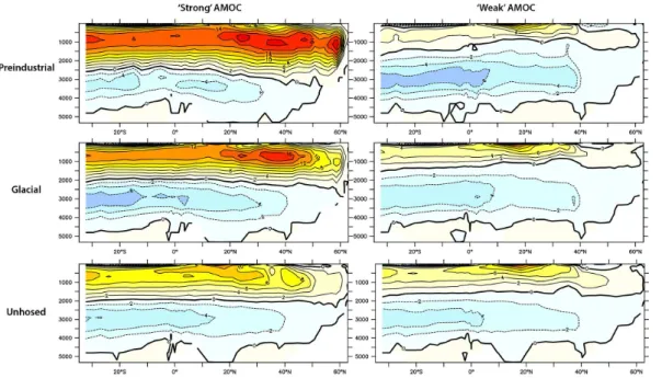
the maximum rate of sea level rise during the last deglaciation (Melt Water Pulse 1a) (Deschamps et al., 2012). For the top panels of Figs. 2–7, the “weak” AMOC state is defined as years 901–1000 of hosing, and the “strong” AMOC state is the same cen-tury taken from the corresponding control simulation to correct for drift, which was quite small.

5

In addition, we show results from a simulation for which hosing was not applied, but which exhibits spontaneous oscillations in the AMOC reminiscent of D-O events, very similar to those of Peltier and Vettoretti (2014). This “Unhosed” simulation was con-ducted under glacial CO₂(180 ppm), but with preindustrial ice sheets and bathymetry, low obliquity, and weak boreal seasonality. The final experiment is a modification of

10

the Unhosed simulation, in which a small (0.05 Sv) hosing is applied during a strong-AMOC interval. This final experiment provides an explicit test of the effect of a hosed vs. an unhosed AMOC weakening.

3 Results

3.1 Simulated changes in the North Atlantic

15

The eight hosed simulations show a number of common features in the North Atlantic, which vary as a function of boundary conditions (Fig. 1). Within the first two centuries of hosing, the Greenland temperature rapidly drops by 8–15◦_{C, with a stronger response}

under high obliquity. When the hosing is stopped, the temperatures abruptly increase by 8–20◦_{C, with a stronger response under high obliquity, and under glacial conditions.}

20

The simulated magnitudes of warming and cooling are of the same magnitude as re-constructed for abrupt climate change from Greenland ice cores (Buizert et al., 2014). The AMOC follows a very similar temporal progression in all cases, which is the inverse of the sea ice extent in the North Atlantic. The average North Atlantic sea surface salin-ity drops by 2–4 PSU in the hosed simulations, consistent with the generally-accepted

25

(8)

CPD

11, 4669–4700, 2015

Title Page

Tables Figures

◭ ◮

Back Close

Full Screen / Esc

Discussion

P

a

per

|

Discussion

P

a

per

|

Discussion

P

a

per

|

Discussion

P

a

per

|

expansion of sea ice, being the cause of an AMOC interruption. Thus, as shown by many prior simulations, the hosing response is quite consistent with observations and the idea of iceberg armadas shutting down the AMOC and initiating abrupt climate change (Kageyama et al., 2013; Menviel et al., 2014).

However, Fig. 1 also shows the same metrics of North Atlantic variability for the

5

Unhosed simulation. Under the low CO₂, low obliquity and preindustrial ice-sheets of this simulation, the model’s coupled ocean–atmosphere system adopts a mode of cir-culation whereby the AMOC spontaneously oscillates between 12–15 and 6 Sv, on a centennial timescale (Figs. 1 and 2). Although the amplitude of the variations in the Unhosed simulation tends to be smaller, with a weaker AMOC throughout (Fig. 2), and

10

the timescale of fluctuations tends to be shorter than the imposed forcing of the Hosed simulations, the general relationship between the four variables is quite similar (Fig. 1). Thus, the Unhosed oscillations are also consistent with observational evidence that a strengthened halocline, associated with an expansion of sea ice, were coupled to a weakening of the AMOC – even in the absence of external freshwater forcing. A very

15

similar type of unforced AMOC oscillation was observed recently in the Community Earth System (CESM) model, run at higher resolution, by Peltier and Vettoretti (2014). The Unhosed variability in CM2Mc can be understood as follows. While the AMOC is weak, heat accumulates in the subsurface North Atlantic (500–1500 m) due to the northward transport of heat from the low latitude thermocline, while the strong halocline

20

impedes the downward mixing of cold surface waters. Eventually, the temperature in-version that results from the buildup of heat at depth counteracts the halocline to the point at which the water column can be destabilized. In the model this occurs when a high-salinity anomaly at the sea surface, caused by decadal variability in precipita-tion and evaporaprecipita-tion, as observed in the modern ocean (Glessmer et al., 2014), triggers

25

(9)

CPD

11, 4669–4700, 2015

Title Page

Tables Figures

◭ ◮

Back Close

Full Screen / Esc

Discussion

P

a

per

|

Discussion

P

a

per

|

Discussion

P

a

per

|

Discussion

P

a

per

|

while the winter sea ice retreat allows much more sensible and latent heat release to the atmosphere, so that the Greenland annual average temperature jumps by 10◦_C

within a decade. Over the next decades to centuries, the strong-AMOC state gradually decays back to a state with greater North Atlantic sea-ice, a low AMOC of 6 Sv and cold Greenland temperatures.

5

The coupled ocean–ice–atmospheric oscillations exhibited by the Unhosed simula-tion are quite consistent with the mechanism proposed by Kaspi et al. (2004), using a simple box model, as well as by Dokken et al. (2013) based on observations from the Nordic seas. It is remarkable that the magnitude of the salinity change in the un-forced simulations is on the order of more than 1 PSU, nearly half as much as for the

10

hosing simulation under the same CO₂and orbital configuration (Fig. 1), in spite of the absence of any external sources of freshwater. In accordance with the suggestion of Kaspi et al. (2004); Li (2005); Dokken et al. (2013), and the similar simulation of Peltier and Vettoretti (2014), we propose that this type of nonlinear changes in sea ice extent, and their coupling with the oceanic and atmospheric circulation, are at the essence of

15

abrupt climate change.

Next, we show how the global consequences of changes in the AMOC depend on the question of whether or not they are forced by freshwater addition. We do so by exploring a few key atmospheric and oceanic variables that have well-documented responses to abrupt climate change as recorded by paleoclimate records.

20

3.2 Global atmospheric response

Abrupt climate change was initially identified in ice core proxy records of atmospheric temperature, and subsequently extended to temperature variations recorded in multiple proxies from around the world (Clement and Peterson, 2008). Figure 3 summarizes the global surface air temperature change that occurs in response to our simulated AMOC

25

(10)

CPD

11, 4669–4700, 2015

Title Page

Tables Figures

◭ ◮

Back Close

Full Screen / Esc

Discussion

P

a

per

|

Discussion

P

a

per

|

Discussion

P

a

per

|

Discussion

P

a

per

|

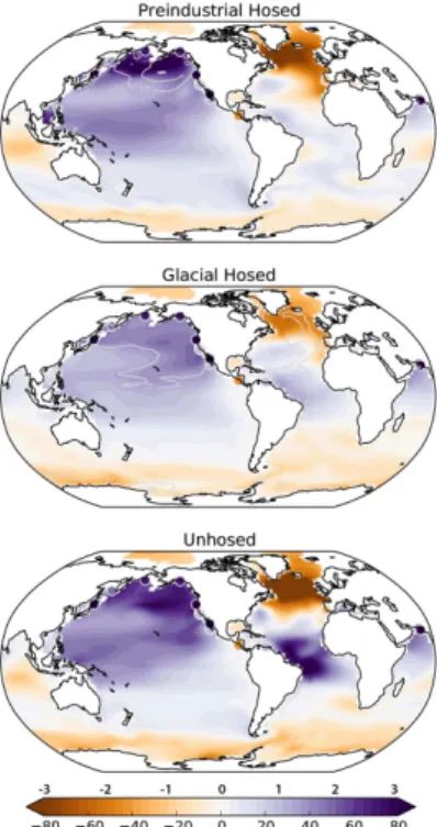
the preindustrial and glacial boundary conditions, as well as in the unhosed simulation. The Northern Hemisphere undergoes general cooling in the extratropics, with greatest cooling in the North Atlantic from Iceland to Iberia, and with cooling extending into the tropics of the eastern Atlantic, North Africa, and southeast Asia. The region of maxi-mum cooling in the Pacific occurs at the Kuroshio-Oyashio confluence, consistent with

5

a southward shift in the front. Meanwhile, the Southern Hemisphere warms everywhere except in the western tropical Pacific and Indian oceans. The maximum warming occurs at high latitudes of the Southern Ocean, and is associated with a sea ice retreat. The general temperature pattern is consistent with the idea of a bipolar seesaw (Broecker, 1998; Stocker and Johnsen, 2003).

10

One notable difference in the spatial patterns is the temperature change in the NE Pacific, including the western margin of Canada and southern Alaska. The tempera-ture here is quite sensitive to the degree of northward transport of warm ocean water from the subtropical gyre, which is quite variable between simulations. All preindustrial hosed simulations develop a strong Pacific Meridional Overturning Circulation (PMOC)

15

when the AMOC weakens, previously described in models as an Atlantic-Pacific See-saw (Saenko et al., 2004; Okumura et al., 2009; Okazaki et al., 2010; Chikamoto et al., 2012; Hu et al., 2012). The development of a strong PMOC counteracts the hemisphere-wide cooling in the NE Pacific, which can actually cause a warming. This suggests that temperature proxy records from this region would provide strong

obser-20

vational constraints on the degree to which a PMOC developed during abrupt climate changes.

The response to hosing in the North Atlantic is particularly dependant on orbital con-figurations in glacial simulations because of different initial sea-ice extents which are strongly driven by obliquity (standard deviation in Fig. 3 and Supplement Fig. 1).

Oth-25

erwise, the response in glacial and preindustrial conditions is fairly consistent between the four extrema orbital configurations.

(11)

CPD

11, 4669–4700, 2015

Title Page

Tables Figures

◭ ◮

Back Close

Full Screen / Esc

Discussion

P

a

per

|

Discussion

P

a

per

|

Discussion

P

a

per

|

Discussion

P

a

per

|

overall patterns of change are similar between Hosed and Unhosed simulations, as they were for the changes in temperature, including reduced precipitation in the North Atlantic, a southward shift of the Intertropical Convergence Zone (ITCZ), and reduced precipitation over south Asia. In fact, many aspects of the precipitation changes vary more as a function of background climate state, including orbital configuration, than

5

they do between Hosed and Unhosed. The two most notable differences between the simulations are the pattern of change surrounding the west Pacific warm pool, an ex-tremely dynamic region with heavy precipitation, and the NE Pacific, where changes in precipitation follow the sea surface temperature through its control on water moisture content and atmospheric circulation. The west Pacific warm pool is an area whose

re-10

sponse to hosing is strongly dependant on orbital configuration (standard deviation in Fig. 4), mostly precession (Supplement Fig. 2).

3.3 Global ocean biogeochemistry response

The observed footprint of abrupt climate change also extends to ocean biogeochem-istry, with pronounced and well-documented changes in both dissolved oxygen

con-15

centrations and export production. Prior work has shown that many aspects of the ob-served oxygenation changes (Schmittner et al., 2007b) and export production changes (Schmittner, 2005; Mariotti et al., 2012) can be well reproduced by coupled ocean-biogeochemistry models under hosing experiments.

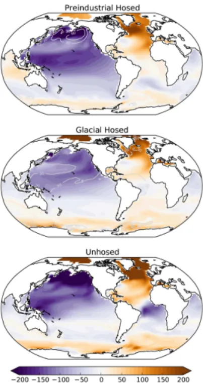
As shown by Fig. 5, our model simulations produce consistent changes in

20

intermediate-depth oxygen during AMOC weakening, hosed or unhosed, that agree well with the bipolar seesaw-mode changes in oxygenation extracted from sediment proxy records of the last deglaciation by Galbraith and Jaccard (2015). All simulations show a decrease of oxygen throughout the full depth of the North Atlantic, due to the lack of ventilated North Atlantic Deep Water, and an increase in the oxygenation of

25

(12)

strongly-CPD

11, 4669–4700, 2015

Title Page

Tables Figures

◭ ◮

Back Close

Full Screen / Esc

Discussion

P

a

per

|

Discussion

P

a

per

|

Discussion

P

a

per

|

Discussion

P

a

per

|

ventilated thermocline impinges on the California margin. This hotspot implies that a tendency for a frontal shift to occur in this region makes it particularly sensitive to changes in the AMOC, and explains why the California borderlands region has such rich records of oxygenation changes on millennial timescales.

As shown by Fig. 6, the simulated changes in the North Pacific and Arabian Sea are

5

driven by large changes in ventilation, that overcome basin-wide changes in export pro-duction (Fig. 7) acting in the opposite direction (i.e. greater export when intermediate-depth oxygen is higher). The primary discrepancies between the simulations are in the degree of oxygen enrichment in the subarctic Pacific, again related to the development of a PMOC, the changes in ventilation in the Tropical Atlantic thermocline, and in the

10

degree of ventilation changes in the Southern Ocean.

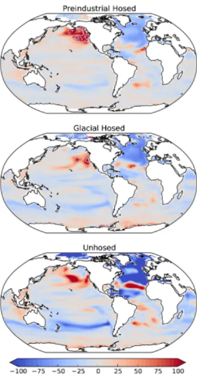
The relative changes in export production, shown in Fig. 7, are locally quite large (in excess of 100 %) but have weaker regional patterns that are less consistent be-tween simulations. The most consistent strong features are a reduction of export in the northern North Atlantic, the western tropical North Atlantic, and the southern margin

15

of the Indo-Pacific subtropical gyre, and an increase in export offof NW Africa, to the west of California, and in the high latitude Southern Ocean. Regions that do not always respond consistently are the subarctic Pacific, which depends significantly on whether or not a PMOC develops, and the Pakistani margin and eastern tropical Pacific, which both show an increase in export under hosing as observed by Kienast et al. (2006)

20

except under glacial hosing, when they do not change. In general, the di_fferences be-tween the various hosed simulations is as large as the difference between hosed and unhosed.

3.4 Hosing the unhosed

The analyses above suggest that the large-scale responses of climate and ocean

bio-25

(13)

CPD

11, 4669–4700, 2015

Title Page

Tables Figures

◭ ◮

Back Close

Full Screen / Esc

Discussion

P

a

per

|

Discussion

P

a

per

|

Discussion

P

a

per

|

Discussion

P

a

per

|

AMOC weakening, we applied a freshwater forcing during a strong AMOC interval of the Unhosed simulation, forcing the model to return to its weak AMOC state earlier than in the standard Unhosed case. This experiment provides a direct comparison be-tween an unforced and a freshwater forced AMOC reduction. The freshwater forcing weakens the AMOC transport (Fig. 1), and maintains its weakened state over the full

5

1000 year simulation, whereas the Unhosed simulation returned to the strong-AMOC state after about 800 years. By comparing both the forced and unforced simulations after 800 years stadial, we can estimate the di_fferences caused by the freshwater itself (Fig. 8).

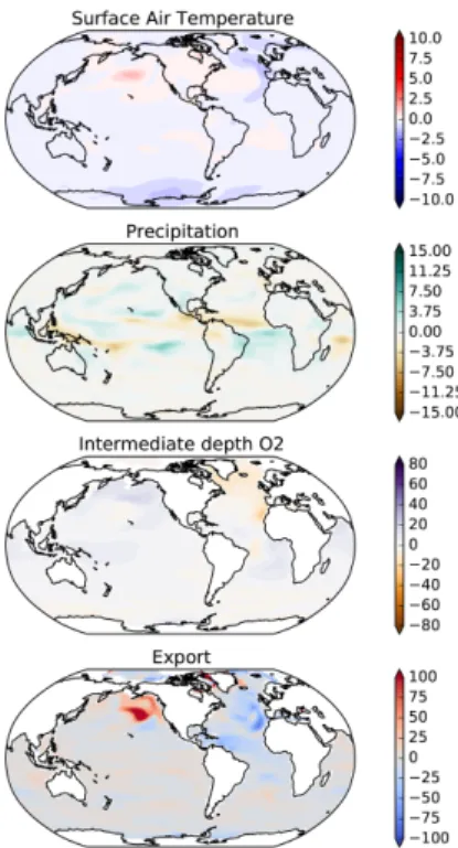
As shown, the changes caused by freshwater itself are quite small compared to the

10

overall changes (compare Fig. 8 with Figs. 3–7 and Supplement Figs. 1–4). Surface air temperatures only differ significantly in the North Atlantic, North Pacific, and high latitude Southern Ocean, while precipitation and oxygen generally show an amplifica-tion of the Unhosed trends, and export producamplifica-tion shows minimal changes except for the N Atlantic and NE Pacific. Most of these di_fferences can be understood by the fact

15

that the freshwater-forced simulation has a slightly weaker AMOC, and more extensive North Atlantic sea-ice coverage, leading to slightly lower temperatures in the NE At-lantic and a correspondingly greater response in atmospheric circulation that amplifies most features of the weak-AMOC state.

Apart from the small amplification of the general trends, we note one distinct

addi-20

tional feature: the Antarctic temperature response is decreased under hosing, weak-ening the bipolar seesaw. This feature of the Antarctic response appears to reflect the transport of freshwater from the North Atlantic to the Southern Ocean through relatively shallow pathways in the Atlantic, so that it freshens the Southern Ocean surface. The addition of freshwater strengthens the Southern Ocean halocline, reducing ocean heat

25

(14)

CPD

11, 4669–4700, 2015

Title Page

Tables Figures

◭ ◮

Back Close

Full Screen / Esc

Discussion

P

a

per

|

Discussion

P

a

per

|

Discussion

P

a

per

|

Discussion

P

a

per

|

(2007a) found an opposite effect of freshwater input on the Southern Ocean, with a rel-ative weakening of the halocline causing a destratification of the Southern Ocean under freshwater forcing. It would thus appear that this aspect of hosing is quite sensitive to model behaviour and experimental design. Given the importance of Southern Ocean convection on controlling atmospheric CO₂(Sarmiento and Toggweiler, 1984; Sigman

5

et al., 2010; Bernardello et al., 2014), this is not a trivial finding.

4 Discussion and conclusions

Our Unhosed model simulation adds to a small, but growing subset of complex 3-dimensional ocean–atmosphere model simulations exhibiting unforced oscillations sim-ilar to the abrupt climate changes of Dansgaard-Oeschger cycles. Under a particular

10

set of boundary conditions (low CO₂, with preindustrial ice sheets and low obliquity), it can spontaneously switch to a much weaker state, triggered by internal climate vari-ability within the model, acting on a type of “salt oscillator”. This model behavior is essentially identical to that described by Peltier and Vettoretti (2014) and Vettoretti and Peltier (2015).

15

These spontaneous AMOC variations suggest that when the AMOC is in a weak state due to the background climate state, it is easy for it to switch into an o_ffmode with very little forcing. Under these conditions, large volcanic eruptions (Pausata et al., 2015), ice-sheet topography changes (Zhang et al., 2014) or ocean–atmosphere cli-mate variability controlling precipitation in the North Atlantic, would be su_fficient to

trig-20

ger an abrupt change. However, the ubiquitous weakening of the AMOC that occurs in models under sufficient hosing implies that, even in a strong mode, the AMOC is vulnerable to freshwater forcing, if it is large enough.

As previously suggested, melting of ice shelves could provide an important feedback to an initial AMOC weakening, accelerating ice sheet mass loss due to their

buttressing-25

(15)

CPD

11, 4669–4700, 2015

Title Page

Tables Figures

◭ ◮

Back Close

Full Screen / Esc

Discussion

P

a

per

|

Discussion

P

a

per

|

Discussion

P

a

per

|

Discussion

P

a

per

|

2011). Such a behaviour is similar to that exhibited here by the Hosed-Unhosed simu-lation, and may have been necessary to produce a complete “shutdown” of the AMOC, as suggested by Pa/Th measurements at Bermuda Rise (Böhm et al., 2015). This sug-gests that the question of whether or not a Heinrich event occurred during an AMOC interruption had more to do with the susceptibility of the Laurentide ice sheet to

col-5

lapse than the nature of the initial AMOC interruption itself. In turn, the degree to which consequent ice sheet melting altered ocean circulation may have depended on where the freshwater was discharged, including how much of the freshwater was input to the ocean as sediment-laden hyperpycnal flows (Tarasov and Peltier, 2005; Roche et al., 2007).

10

Although they only occur in our model under an unrealistic combination of boundary conditions, a fact which is likely sensitive to the parameterization of deep ocean mix-ing (Peltier and Vettoretti, 2014), the spontaneous nature of these oscillations allows a powerful comparison to be made with the more typical freshwater-hosed simulations of AMOC weakening. When compared with the Hosed simulations, the general

fea-15

tures of the atmospheric and oceanic responses are remarkably robust. These robust features can therefore be taken to reflect consistent dynamical changes related to the AMOC interruption and its coupling with sea ice and atmospheric changes, indepen-dent of the ultimate cause of the AMOC interruption. The only substantial difference noted between Hosed and Unhosed simulations lay in the direct impact of freshwater

20

on ocean density structure. The injection of freshwater in the North Atlantic can quickly spread throughout the global ocean, dependent on the distribution of its input and the ocean circulation pattern. In our simulations, the most important consequence of this is the stratification of the Southern Ocean, which is intensified by the freshwater ini-tially injected to the North Atlantic. Aside from this relatively minor contrast, the global

25

(16)

CPD

11, 4669–4700, 2015

Title Page

Tables Figures

◭ ◮

Back Close

Full Screen / Esc

Discussion

P

a

per

|

Discussion

P

a

per

|

Discussion

P

a

per

|

Discussion

P

a

per

|

The Supplement related to this article is available online at doi:10.5194/cpd-11-4669-2015-supplement.

Acknowledgements. We thank the Canadian Foundation for Innovation (CFI) and an allocation to the Scinet supercomputing facility (University of Toronto), made through Compute Canada, for providing the computational resources. We are also grateful towards the open-source

com-5

munities behind the development of all the python libraries used to create the graphics for this article, particularly Matplotlib (Hunter, 2007) and Cartopy (MetOffice).

References

Alley, R. B., Marotzke, J., Nordhaus, W. D., Overpeck, J. T., Peteet, D. M., Pielke, R. A., Pierre-humbert, R. T., Rhines, P. B., Stocker, T. F., Talley, L. D., and Wallace, J. M.: Abrupt climate

10

change, Science, 299, 2005–2010, doi:10.1126/science.1081056, 2003. 4670

Alvarez-Solas, J., Charbit, S., Ritz, C., Paillard, D., Ramstein, G., and Dumas, C.: Links between ocean temperature and iceberg discharge during Heinrich events, Nat. Geosci., 3, 122–126, doi:10.1038/ngeo752, 2010. 4672, 4682

Anderson, J. L.: The new GFDL Global Atmosphere and Land Model AM2-LM2: evaluation

15

with prescribed SST simulations, J. Climate, 17, 4641–4673, doi:10.1175/JCLI-3223.1, 2004. 4673

Barker, S., Chen, J., Gong, X., Jonkers, L., Knorr, G., and Thornalley, D.: Icebergs not the trigger for North Atlantic cold events, Nature, 520, 333–336, doi:10.1038/nature14330, doi:10.1038/nature14330, 2015. 4672

20

Bernardello, R., Marinov, I., Palter, J. B., Galbraith, E. D., and Sarmiento, J. L.: Impact of Wed-dell Sea deep convection on natural and anthropogenic carbon in a climate model, Geophys. Res. Lett., 41, 7262–7269, doi:10.1002/2014GL061313, 2014. 4682

Böhm, E., Lippold, J., Gutjahr, M., Frank, M., Blaser, P., Antz, B., Fohlmeister, J., Frank, N., An-dersen, M. B., and Deininger, M.: Strong and deep Atlantic meridional overturning circulation

25

during the last glacial cycle, Nature, 517, 73–76, doi:10.1038/nature14059, 2015. 4683 Broecker, W. S.: Massive iceberg discharges as triggers for global climate change, Nature, 372,

(17)

CPD

11, 4669–4700, 2015

Title Page

Tables Figures

◭ ◮

Back Close

Full Screen / Esc

Discussion

P

a

per

|

Discussion

P

a

per

|

Discussion

P

a

per

|

Discussion

P

a

per

|

Broecker, W. S.: Paleocean circulation during the last deglaciation: a bipolar seesaw?, Paleo-ceanography, 13, 119–121, doi:10.1029/97PA03707, 1998. 4678

Buizert, C., Gkinis, V., Severinghaus, J. P., He, F., Lecavalier, B. S., Kindler, P., Leuenberger, M., Carlson, A. E., Vinther, B., Masson-Delmotte, V., White, J. W. C., Liu, Z., Otto-Bliesner, B., and Brook, E. J.: Greenland temperature response to climate forcing during the last

deglacia-5

tion, Science, 345, 1177–1180, doi:10.1126/science.1254961, 2014. 4675

Chikamoto, M. O., Menviel, L., Abe-Ouchi, A., Ohgaito, R., Timmermann, A., Okazaki, Y., Harada, N., Oka, A., and Mouchet, A.: Variability in North Pacific intermediate and deep water ventilation during Heinrich events in two coupled climate models, Deep-Sea Res. Pt. II, 61–64, 114–126, doi:10.1016/j.dsr2.2011.12.002, 2012. 4678

10

Clark, P. U., Pisias, N. G., Stocker, T. F., and Weaver, A. J.: The role of the thermoha-line circulation in abrupt climate change, Nature, 415, 863–869, doi:10.1038/415863a, doi:10.1038/415863a, 2002. 4670

Clement, A. C. and Peterson, L. C.: Mechanisms of abrupt climate change of the last glacial period, Rev. Geophys., 46, RG4002, doi:10.1029/2006RG000204, 2008. 4670, 4677

15

Dansgaard, W., Johnsen, S. J., Clausen, H. B., Dahl-Jensen, D., Gundestrup, N. S., Ham-mer, C. U., Hvidberg, C. S., Steffensen, J. P., Sveinbjornsdottir, A. E., Jouzel, J., and Bond, G.: Evidence for general instability of past climate from a 250-kyr ice-core record, Nature, 364, 218–220, doi:10.1038/364218a0, 1993. 4672

Deschamps, P., Durand, N., Bard, E., Hamelin, B., Camoin, G., Thomas, A. L.,

Hen-20

derson, G. M., Okuno, J., and Yokoyama, Y.: Ice-sheet collapse and sea-level rise at the Bolling warming 14600 years ago, Nature, 483, 559–564, doi:10.1038/nature10902, doi:10.1038/nature10902, 2012. 4675

Dokken, T. M., Nisancioglu, K. H., Li, C., Battisti, D. S., and Kissel, C.: Dansgaard-Oeschger cy-cles: Interactions between ocean and sea ice intrinsic to the Nordic seas, Paleoceanography,

25

28, 491–502, doi:10.1002/palo.20042, 2013. 4677

Drijfhout, S., Gleeson, E., Dijkstra, H. A., and Livina, V.: Spontaneous abrupt climate change due to an atmospheric blocking-sea-ice-ocean feedback in an unforced climate model simu-lation, P. Natl. Acad. Sci. USA, 110, 19713–8, doi:10.1073/pnas.1304912110, 2013. 4671 Dunne, J. P., John, J. G., Adcroft, A. J., Griffies, S. M., Hallberg, R. W., Shevliakova, E.,

30

(18)

CPD

11, 4669–4700, 2015

Title Page

Tables Figures

◭ ◮

Back Close

Full Screen / Esc

Discussion

P

a

per

|

Discussion

P

a

per

|

Discussion

P

a

per

|

Discussion

P

a

per

|

models. Part I: Physical formulation and baseline simulation characteristics, J. Climate, 25, 6646–6665, doi:10.1175/JCLI-D-11-00560.1, 2012. 4673

Fanning, A. F. and Weaver, A. J.: Temporal-geographical meltwater influences on the North Atlantic conveyor: implications for the Younger Dryas, Paleoceanography, 12, 307–320, doi:10.1029/96PA03726, 1997. 4671

5

Flückiger, J., Knutti, R., and White, J. W. C.: Oceanic processes as potential trig-ger and amplifying mechanisms for Heinrich events, Paleoceanography, 21, PA2014, doi:10.1029/2005PA001204, 2006. 4672

Friedrich, T., Timmermann, A., Menviel, L., Elison Timm, O., Mouchet, A., and Roche, D. M.: The mechanism behind internally generated centennial-to-millennial scale climate

variabil-10

ity in an earth system model of intermediate complexity, Geosci. Model Dev., 3, 377–389, doi:10.5194/gmd-3-377-2010, 2010. 4671

Galbraith, E. D. and Jaccard, S. L.: Deglacial weakening of the oceanic soft tissue pump: global constraints from sedimentary nitrogen isotopes and oxygenation proxies, Quaternary Sci. Rev., 109, 38–48, doi:10.1016/j.quascirev.2014.11.012, 2015. 4679, 4697

15

Galbraith, E. D., Gnanadesikan, A., Dunne, J. P., and Hiscock, M. R.: Regional impacts of iron-light colimitation in a global biogeochemical model, Biogeosciences, 7, 1043–1064, doi:10.5194/bg-7-1043-2010, 2010. 4673

Galbraith, E. D., Kwon, E. U. N. Y., Gnanadesikan, A., Rodgers, K. B., Griffies, S. M., Bianchi, D., Sarmiento, J. L., Dunne, J. P., Simeon, J., Slater, R. D., Wittenberg, A. T., and Held, I. M.:

20

Climate variability and radiocarbon in the CM2Mc earth system model, J. Climate, 24, 4230– 4254, doi:10.1175/2011JCLI3919.1, 2011. 4673, 4674

Ganopolski, A. and Rahmstorf, S.: Rapid changes of glacial climate simulated in a coupled climate model, Nature, 409, 153–158, 2001. 4671

Ganopolski, A. and Rahmstorf, S.: Abrupt glacial climate changes due to stochastic resonance,

25

Phys. Rev. Lett., 88, 038501, doi:10.1103/PhysRevLett.88.038501, 2002. 4671

Glessmer, M. S., Eldevik, T., Vå ge, K., Øie Nilsen, J. E., and Behrens, E.: Atlantic origin of observed and modelled freshwater anomalies in the Nordic Seas, Nat. Geosci., 7, 801–805, doi:10.1038/ngeo2259, 2014. 4676

Gong, X., Knorr, G., Lohmann, G., and Zhang, X.: Dependence of abrupt Atlantic meridional

30

(19)

CPD

11, 4669–4700, 2015

Title Page

Tables Figures

◭ ◮

Back Close

Full Screen / Esc

Discussion

P

a

per

|

Discussion

P

a

per

|

Discussion

P

a

per

|

Discussion

P

a

per

|

Gutjahr, M. and Lippold, J.: Early arrival of Southern Source Water in the deep North Atlantic prior to Heinrich event 2, Paleoceanography, 26, PA2101, doi:10.1029/2011PA002114, 2011. 4672

Hall, A. and Stouffer, R. J.: An abrupt climate event in a coupled ocean–atmosphere simulation without external forcing, Nature, 409, 171–174, doi:10.1038/35051544, 2001. 4671

5

Harrison, S., and Sanchez Goñi, M.: Global patterns of vegetation response to millennial-scale variability and rapid climate change during the last glacial period, Quaternary Sci. Rev., 29, 2957–2980, doi:10.1016/j.quascirev.2010.07.016, 2010. 4671

Heinrich, H.: Origin and consequences of cyclic ice rafting in the Northeast Atlantic Ocean during the past 130,000 years, Quaternary Res., 29, 142–152,

doi:10.1016/0033-10

5894(88)90057-9, 1988. 4671

Hemming, S. R.: Heinrich events: massive late Pleistocene detritus layers of the North Atlantic and their global climate imprint, Rev. Geophys., 42, RG1005, doi:10.1029/2003RG000128, 2004. 4672

Hu, A., Otto-Bliesner, B. L., Meehl, G. A., Han, W., Morrill, C., Brady, E. C., and Briegleb, B.:

15

Response of thermohaline circulation to freshwater forcing under present-day and LGM con-ditions, J. Climate, 21, 2239–2258, doi:10.1175/2007JCLI1985.1, 2008. 4671

Hu, A., Meehl, G. A., Han, W., Abe-Ouchi, A., Morrill, C., Okazaki, Y., and Chikamoto, M. O.: The Pacific-Atlantic seesaw and the Bering Strait, Geophys. Res. Lett., 39, L03702, doi:10.1029/2011GL050567, 2012. 4678

20

Hunter, J. D.: Matplotlib: a 2D graphics environment, Comput. Sci. Eng., 9, 90–95, 2007. 4684 Kageyama, M., Merkel, U., Otto-Bliesner, B., Prange, M., Abe-Ouchi, A., Lohmann, G., Ohgaito, R., Roche, D. M., Singarayer, J., Swingedouw, D., and X Zhang: Climatic impacts of fresh water hosing under Last Glacial Maximum conditions: a multi-model study, Clim. Past, 9, 935–953, doi:10.5194/cp-9-935-2013, 2013. 4671, 4676

25

Kaspi, Y., Sayag, R., and Tziperman, E.: A “triple sea-ice state” mechanism for the abrupt warming and synchronous ice sheet collapses during Heinrich events, Paleoceanography, 19, PA3004, doi:10.1029/2004PA001009, 2004. 4677

Kienast, M., Kienast, S. S., Calvert, S. E., Eglinton, T. I., Mollenhauer, G., François, R., and Mix, A. C.: Eastern Pacific cooling and Atlantic overturning circulation during the last

30

deglaciation, Nature, 443, 846–849, doi:10.1038/nature05222, 2006. 4680

(20)

CPD

11, 4669–4700, 2015

Title Page

Tables Figures

◭ ◮

Back Close

Full Screen / Esc

Discussion

P

a

per

|

Discussion

P

a

per

|

Discussion

P

a

per

|

Discussion

P

a

per

|

Africa during Dansgaard–Oeschger interstadials, Earth Planet. Sc. Lett., 339–340, 95–102, doi:10.1016/j.epsl.2012.05.018, 2012. 4671

Krebs, U. and Timmermann, A.: Tropical air–sea interactions accelerate the recovery of the Atlantic meridional overturning circulation after a major shutdown, J. Climate, 20, 4940– 4956, doi:10.1175/JCLI4296.1, 2007. 4671

5

Laskar, J., Robutel, P., Joutel, F., Gastineau, M., Correia, A. C. M., and Levrard, B.: A long-term numerical solution for the insolation quantities of the Earth, Astron. Astrophys., 428, 261–285, doi:10.1051/0004-6361:20041335, 2004. 4674

Li, C.: Abrupt climate shifts in Greenland due to displacements of the sea ice edge, Geophys. Res. Lett., 32, L19702, doi:10.1029/2005GL023492, 2005. 4671, 4677

10

Li, C., Battisti, D. S., and Bitz, C. M.: Can North Atlantic sea ice anoma-lies account for Dansgaard–Oeschger climate signals?, J. Climate, 23, 5457–5475, doi:10.1175/2010JCLI3409.1, 2010. 4671

Liu, Z., Otto-Bliesner, B. L., He, F., Brady, E. C., Tomas, R., Clark, P. U., Carlson, A. E., Lynch-Stieglitz, J., Curry, W., Brook, E., Erickson, D., Jacob, R., Kutzbach, J., and Cheng, J.:

Tran-15

sient simulation of last deglaciation with a new mechanism for Bolling-Allerod warming, Sci-ence, 325, 310–314, doi:10.1126/science.1171041, 2009. 4671

Loving, J. L. and Vallis, G. K.: Mechanisms for climate variability during glacial and interglacial periods, Paleoceanography, 20, PA4024, doi:10.1029/2004PA001113, 2005. 4671

MacAyeal, D. R.: Binge/purge oscillations of the laurentide ice sheet as a cause of the North

20

Atlantic’s Heinrich events, Paleoceanography, 8, 775–784, doi:10.1029/93PA02200, 1993. 4671

Marcott, S. A., Clark, P. U., Padman, L., Klinkhammer, G. P., Springer, S. R., Liu, Z., Otto-Bliesner, B. L., Carlson, A. E., Ungerer, A., Padman, J., He, F., Cheng, J., and Schmittner, A.: Ice-shelf collapse from subsurface warming as a trigger for Heinrich events, P. Natl. Acad.

25

Sci. USA, 108, 13415–13419, doi:10.1073/pnas.1104772108, 2011. 4672, 4682

Mariotti, V., Bopp, L., Tagliabue, A., Kageyama, M., and Swingedouw, D.: Marine produc-tivity response to Heinrich events: a model-data comparison, Clim. Past, 8, 1581–1598, doi:10.5194/cp-8-1581-2012, 2012. 4679

Marshall, S. J. and Koutnik, M. R.: Ice sheet action versus reaction: distinguishing between

30

(21)

CPD

11, 4669–4700, 2015

Title Page

Tables Figures

◭ ◮

Back Close

Full Screen / Esc

Discussion

P

a

per

|

Discussion

P

a

per

|

Discussion

P

a

per

|

Discussion

P

a

per

|

Menviel, L., Timmermann, A., Friedrich, T., and England, M. H.: Hindcasting the continuum of Dansgaard–Oeschger variability: mechanisms, patterns and timing, Clim. Past, 10, 63–77, doi:10.5194/cp-10-63-2014, 2014. 4671, 4676

MetOffice: Cartopy: a cartographic python library with a matplotlib interface, Exeter, Devon, available at: http://scitools.org.uk/cartopy, May 2015. 4684

5

Mignot, J., Ganopolski, A., and Levermann, A.: Atlantic subsurface temperatures: response to a shutdown of the overturning circulation and consequences for its recovery, J. Climate, 20, 4884–4898, doi:10.1175/JCLI4280.1, 2007. 4672

Okazaki, Y., Timmermann, A., Menviel, L., Harada, N., Abe-Ouchi, A., Chikamoto, M. O., Mouchet, A., and Asahi, H.: Deepwater formation in the North Pacific during the last glacial

10

termination, Science, 329, 200–204, doi:10.1126/science.1190612, 2010. 4678

Okumura, Y. M., Deser, C., Hu, A., Timmermann, A., and Xie, S.-P.: North Pacific climate re-sponse to freshwater forcing in the subarctic North Atlantic: oceanic and atmospheric path-ways, J. Climate, 22, 1424–1445, doi:10.1175/2008JCLI2511.1, 2009. 4678

Otto-Bliesner, B. L. and Brady, E. C.: The sensitivity of the climate response to the magnitude

15

and location of freshwater forcing: last glacial maximum experiments, Quaternary Sci. Rev., 29, 56–73, doi:10.1016/j.quascirev.2009.07.004, 2010. 4671

Pausata, F. S. R., Grini, A., Caballero, R., Hannachi, A., and Seland, O. y.: High-latitude volcanic eruptions in the Norwegian Earth System Model: the effect of different initial conditions and of the ensemble size, Tellus B, 67, doi:10.3402/tellusb.v67.26728, 2015. 4682

20

Peltier, W. R. and Vettoretti, G.: Dansgaard-Oeschger oscillations predicted in a comprehensive model of glacial climate: a “kicked” salt oscillator in the Atlantic, Geophys. Res. Lett., 41, 7306–7313, doi:10.1002/2014GL061413, 2014. 4671, 4675, 4676, 4677, 4682, 4683 Petersen, S. V., Schrag, D. P., and Clark, P. U.: A new mechanism for Dansgaard–Oeschger

cycles, Paleoceanography, 28, 24–30, doi:10.1029/2012PA002364, 2013. 4671

25

Rahmstorf, S., Crucifix, M., Ganopolski, A., Goosse, H., Kamenkovich, I., Knutti, R., Lohmann, G., Marsh, R., Mysak, L. A., Wang, Z., and Weaver, A. J.: Thermoha-line circulation hysteresis: a model intercomparison, Geophys. Res. Lett., 32, L23605, doi:10.1029/2005GL023655, 2005. 4671

Roberts, W. H. G., Valdes, P. J., and Payne, A. J.: Topography’s crucial role in Heinrich Events,

30

(22)

CPD

11, 4669–4700, 2015

Title Page

Tables Figures

◭ ◮

Back Close

Full Screen / Esc

Discussion

P

a

per

|

Discussion

P

a

per

|

Discussion

P

a

per

|

Discussion

P

a

per

|

Roche, D. M., Renssen, H., Weber, S. L., and Goosse, H.: Could meltwater pulses have been sneaked unnoticed into the deep ocean during the last glacial?, Geophys. Res. Lett., 34, L24708, doi:10.1029/2007GL032064, 2007. 4683

Saenko, O. A., Schmittner, A., and Weaver, A. J.: The Atlantic – Pacific seesaw, J. Climate, 17, 2033–2038, 2004. 4678

5

Sakai, K. and Peltier, W. R.: Dansgaard–Oeschger oscillations in a coupled atmosphere–ocean climate model, J. Climate, 10, 949–970, doi:10.1175/1520-0442(1997)010<0949:DOOIAC>2.0.CO;2, 1997. 4671

Sarmiento, J. L. and Toggweiler, J. R.: A new model for the role of the oceans in determining atmospheric PCO2, Nature, 308, 621–624, doi:10.1038/308621a0, 1984. 4682

10

Schmittner, A.: Decline of the marine ecosystem caused by a reduction in the Atlantic overturn-ing circulation, Nature, 434, 628–633, doi:10.1038/nature03476, 2005. 4679

Schmittner, A. and Galbraith, E. D.: Glacial greenhouse-gas fluctuations controlled by ocean circulation changes, Nature, 456, 373–376, doi:10.1038/nature07531, 2008. 4671

Schmittner, A., Brooke, E., and Ahn, J.: Impact of the ocean’s overturning circulation on

atmo-15

spheric CO2, in: Ocean Circulation: Mechanisms and Impacts, vol. 173, AGU Geoph. Monog. Series, American Geophysical Union, 209–246, 2007a. 4681

Schmittner, A., Galbraith, E. D., Hostetler, S. W., Pedersen, T. F., and Zhang, R.: Large fluc-tuations of dissolved oxygen in the Indian and Pacific oceans during Dansgaard–Oeschger oscillations caused by variations of North Atlantic deep water subduction, Paleoceanography,

20

22, PA3207, doi:10.1029/2006PA001384, 2007b. 4679

Schulz, M.: Relaxation oscillators in concert: a framework for climate change at millennial timescales during the late Pleistocene, Geophys. Res. Lett., 29, 2193, doi:10.1029/2002GL016144, 2002. 4671

Shaffer, G.: Ocean subsurface warming as a mechanism for coupling Dansgaard–

25

Oeschger climate cycles and ice-rafting events, Geophys. Res. Lett., 31, L24202, doi:10.1029/2004GL020968, 2004. 4672

Siddall, M., Rohling, E. J., Blunier, T., and Spahni, R.: Patterns of millennial variability over the last 500 ka, Clim. Past, 6, 295–303, doi:10.5194/cp-6-295-2010, 2010. 4671

Sigman, D. M., Hain, M. P., and Haug, G. H.: The polar ocean and glacial cycles in atmospheric

30

CO2concentration, Nature, 466, 47–55, doi:10.1038/nature09149, 2010. 4682

(23)

CPD

11, 4669–4700, 2015

Title Page

Tables Figures

◭ ◮

Back Close

Full Screen / Esc

Discussion

P

a

per

|

Discussion

P

a

per

|

Discussion

P

a

per

|

Discussion

P

a

per

|

Stommel, H.: Thermohaline convection with two stable regimes of flow, Tellus, 13, 224–230, doi:10.1111/j.2153-3490.1961.tb00079.x, 1961. 4671

Stouffer, R. J., Yin, J., Gregory, J. M., Dixon, K. W., Spelman, M. J., Hurlin, W., Weaver, A. J., Eby, M., Flato, G. M., Hasumi, H., Hu, A., Jungclaus, J. H., Kamenkovich, I. V., Lever-mann, A., Montoya, M., Murakami, S., Nawrath, S., Oka, A., Peltier, W. R., Robitaille, D. Y.,

5

Sokolov, A., Vettoretti, G., and Weber, S. L.: Investigating the causes of the response of the thermohaline circulation to past and future climate changes, J. Climate, 19, 1365–1387, doi:10.1175/JCLI3689.1, 2006. 4671

Tarasov, L. and Peltier, W. R.: Arctic freshwater forcing of the Younger Dryas cold reversal, Nature, 435, 662–665, doi:10.1038/nature03617, 2005. 4683

10

Vettoretti, G. and Peltier, W. R.: Interhemispheric air temperature phase relationships in the nonlinear Dansgaard–Oeschger oscillation, Geophys. Res. Lett., 42, 1180–1189, doi:10.1002/2014GL062898, 2015. 4671, 4682

Voelker, A. H.: Global distribution of centennial-scale records for Marine Isotope Stage (MIS) 3: a database, Quaternary Sci. Rev., 21, 1185–1212, doi:10.1016/S0277-3791(01)00139-1,

15

2002. 4670

Wang, Z. and Mysak, L. A.: Glacial abrupt climate changes and Dansgaard–Oeschger oscilla-tions in a coupled climate model, Paleoceanography, 21, 1–9, doi:10.1029/2005PA001238, 2006. 4671

Winton, M.: Deep Decoupling Oscillations of the Oceanic Thermohaline Circulation, in: Ice in

20

the Climate System, Vol. 12, NATO ASI Series, edited by: Richard Peltier, W., Springer Berlin Heidelberg, 417–432, 1993. 4671

(24)

CPD

11, 4669–4700, 2015

Title Page

Tables Figures

◭ ◮

Back Close

Full Screen / Esc

Discussion

P

a

per

|

Discussion

P

a

per

|

Discussion

P

a

per

|

Discussion

P

a

per

(25)

CPD

11, 4669–4700, 2015

Title Page

Tables Figures

◭ ◮

Back Close

Full Screen / Esc

Discussion

P

a

per

|

Discussion

P

a

per

|

Discussion

P

a

per

|

Discussion

P

a

per

|

(26)

CPD

11, 4669–4700, 2015

Title Page

Tables Figures

◭ ◮

Back Close

Full Screen / Esc

Discussion

P

a

per

|

Discussion

P

a

per

|

Discussion

P

a

per

|

Discussion

P

a

per

|

(27)

CPD

11, 4669–4700, 2015

Title Page

Tables Figures

◭ ◮

Back Close

Full Screen / Esc

Discussion

P

a

per

|

Discussion

P

a

per

|

Discussion

P

a

per

|

Discussion

P

a

per

|

(28)

CPD

11, 4669–4700, 2015

Title Page

Tables Figures

◭ ◮

Back Close

Full Screen / Esc

Discussion

P

a

per

|

Discussion

P

a

per

|

Discussion

P

a

per

|

Discussion

P

a

per

|

Figure 4.Stadial precipitation change normalized to a 10 Sv AMOC decrease. The top two panels show the normalized precipitation difference between weak and strong AMOC states (as defined in Fig. 2) under Preindustrial and Glacial boundary conditions, averaged between the four sets of orbital configurations (see Supplement Fig. 2 to view all 8 hosing simulations individually). Grey contours show the standard deviation between the four sets of orbital config-urations at 5×10−6kg m−2s−1intervals. The bottom panel shows the normalized precipitation

(29)

CPD

11, 4669–4700, 2015

Title Page

Tables Figures

◭ ◮

Back Close

Full Screen / Esc

Discussion

P

a

per

|

Discussion

P

a

per

|

Discussion

P

a

per

|

Discussion

P

a

per

|

Figure 5.Stadial intermediate-depth (400–1400 m) oxygen concentration change normalized to a 10 Sv AMOC decrease. The top two panels show the normalized oxygen concentration difference between weak and strong AMOC states (as defined in Fig. 2) under Preindustrial and Glacial boundary conditions, averaged between the four sets of orbital configurations (see Supplement Fig. 3 to view all 8 hosing simulations individually). Light grey contours show the standard deviation between the four sets of orbital configurations at 10×10−6mol kg−1intervals.

(30)

CPD

11, 4669–4700, 2015

Title Page

Tables Figures

◭ ◮

Back Close

Full Screen / Esc

Discussion

P

a

per

|

Discussion

P

a

per

|

Discussion

P

a

per

|

Discussion

P

a

per

|

(31)

CPD

11, 4669–4700, 2015

Title Page

Tables Figures

◭ ◮

Back Close

Full Screen / Esc

Discussion

P

a

per

|

Discussion

P

a

per

|

Discussion

P

a

per

|

Discussion

P

a

per

|

(32)

CPD

11, 4669–4700, 2015

Title Page

Tables Figures

◭ ◮

Back Close

Full Screen / Esc

Discussion

P

a

per

|

Discussion

P

a

per

|

Discussion

P

a

per

|

Discussion

P

a

per

|