Green function for a non-Markovian Fokker-Planck equation: Comb-model and anomalous
diffusion
L. R. da Silva1, A. A. Tateishi2, M. K. Lenzi3, E. K. Lenzi2, and P. C. da Silva1,4
1Departamento de F´ısica and National Institute of Science and Technology for Complex Systems,
Universidade Federal do Rio Grande do Norte, 59072-970, Natal, RN, Brazil
2Departamento de F´ısica and National Institute of Science and Technology for Complex Systems,
Universidade Estadual de Maring´a, Avenida Colombo, 5790, 87020-900, Maring´a, PR, Brazil 3Departamento de Engenharia Qu´ımica, Universidade Federal do Paran´a,
Setor de Tecnologia - Jardim das Am´ericas, Caixa Postal 19011, 81531-990, Curitiba, PR, Brazil 4 Centro Federal de Educac¸˜ao Tecnol´ogica do Rio Grande do Norte,
Av. Sen. Salgado Filho, 1559, 59015-000, Tirol, Natal, RN (Received on 10 February, 2009)
We investigate solutions, by using the Green function approach, for a system governed by a non-Markovian Fokker-Planck equation and subjected to a Comb structure. This structure consists of the axis of structure as the backbone and fingers which are attached perpendicular to the axis. For this system, we consider an arbitrary initial condition, in the presence of time dependent diffusion coefficients and spatial fractional derivative, and analyze the connection to the anomalous diffusion.
Keywords: Anomalous diffusion, Comb-model, Fokker-Planck
1. INTRODUCTION
The existence of several diffusive processes in which the mean-square displacement is not asymptotically linear in time such as micelles dissolved in salted water [1], surface growth and transport of fluid in porous media [2], two dimensional rotating flow[3], subrecoil laser cooling [4], diffusion on frac-tals [5], enhanced diffusion in active intracellular transport [6], particle diffusion in a quasi-two-dimensional bacterial bath [7] has motivated the study of several approaches, in par-ticular, the fractional diffusion equations [8–14] due to the broadness of applications. They have been used to inves-tigate, for example, anomalous transport in disordered sys-tems [15], diffusion on fractals [16], and in non-Markovian dynamical processes in protein folding [17]. This variety of applications of the fractional diffusion equations have stimu-lated the study of several formal aspects such as the behav-ior at the origin [18], the connection with generalized master equation [19], their solutions[20–31] by taking external force and spatial dependent diffusion coefficient into account, the effect produced by reaction terms [32–34], solutions in fined regions with spatial and time dependent boundary con-ditions [35, 36], and the relation between the fractional dif-fusion equations and comb-model [37–42]. In this point, it is also interesting to mention that the comb-model is applied to investigate porous medium related to exploration of low di-mensional percolation clusters, the problem of flow transfer in disordered systems [43], electrophoresis process and tu-mor development [44]. From the above discussion, we note the relevance of these investigations concerning the fractional diffusion equations and the importance of extending these cases to open the wide range of scenarios. In this direction, we dedicated this work to investigate the solutions for an ex-tension of the comb-model which is based on the following non-Markovian diffusion equation:
∂
∂tρ(x,y;t) = Z t
0
dt′
D
y(t−t′)∂2
∂y2ρ(x,y;t′) +δ(y)
Z t
0
dt′
D
x(t−t′)∂µ
∂|x|µρ(x,y;t′) (1)
where
D
y(t)andD
x(t)are time dependent diffusioncoeffi-cients and the fractional derivative applied to the spatial vari-able is the Riesz-Weyl operator [45].
The plan of this work is to investigate Eq. (1) by taking the boundary conditionsρ(±∞,y,t) =0 andρ(x,±∞,t) =0 and the initial condition ρ(x,y,0) =bρ(x,y)into account, where b
ρ(x,y)is how the system is initially distributed and it is nor-malized, i.e.,R−∞∞dxR−∞∞dybρ(x,y) =1. We first consider the case given by
D
y(t) =D
yδ(t),D
x(t) =D
xδ(t)andµ=2. Theresult obtained for this case permits us to show the effect pro-duced by an arbitrary initial condition on the solution. In par-ticular, the spreading of the distribution for initial times where the influence of the initial condition is important. Following, we incorporate a power law dependence for the diffusion co-efficients, i.e.,
D
y(t) =D
ytγy−2/Γ(γy−1)(D
y(s) =D
ys1−γyand 0<γy<1),
D
x(t) =D
xtγx−2/Γ(γx−1)(D
x(s) =D
xs1−γxand 0<γx<1). This time dependence for the diffusion
coef-ficients may be related to the fractional time derivatives and it makes possible to obtain the inverse Laplace transform. An-other time dependence for the diffusion coefficients is possi-ble, however may lead us to cumbersome calculations. Af-terwards, we incorporated spatial fractional derivatives, i.e., µ6=2, in our analysis. For these cases, we obtain the exact solution by using the Green function approach [46] and the dispersion relation when it is defined. These developments are presented in Sec. II and in Sec. III we present our discus-sion and concludiscus-sion about the results found here.
2. NON-MARKOVIAN FOKKER PLANCK EQUATION
Let us start by considering Eq.(1) with
D
y(t) =D
yδ(t),D
x(t) =D
xδ(t)andµ=2. For this case, it is given by∂
∂tρ(x,y,t) =
D
y ∂2∂y2ρ(x,y,t) +
D
xδ(y) ∂2iny=0. A direct consequence of this restriction on the sys-tem is the presence of an anomalous diffusion (subdiffusion) in this direction. This feature may be verified by evaluating the mean square displacement of the solution on the variable x.
We analyze Eq.(2) by accomplishing the boundary con-ditions ρ(±∞,y,t) =0 and ρ(x,±∞,t) = 0 and the initial condition ρ(x,y,0) =bρ(x,y) with R−∞∞dxR−∞∞dyρ(x,y,0) = R∞
−∞dx
R∞
−∞dybρ(x,y) =1, i.e., the distribution is initially
nor-malized. Note that solutions for this equation are obtained by taking a general initial condition into account, in contrast to the cases worked out, for example, in [39–42] which con-sider particular forms for the initial condition. In order to perform this analysis and obtain the solution for this case, we use integrals transforms (Laplace and Fourier) and use the Green function approach. Applying the Fourier transform on thexvariable (
F
{...}=R−∞∞dxe−ikxx... andF
−1{...}=1 2π
R∞
−∞dkxeikxx...) and the Laplace transform on t variable
(
L
{...}=R0∞dte−st... andL
−1{...}= 21πiR−i∞i∞++ccdsest...) in Eq.(2), we obtainD
yd2
dy2ρ(kx,y,s) − s+
D
xk 2xδ(y)
ρ(kx,y,s)
= −ρ(kx,y,0). (3)
This equation may be solved by using the Green function
ap-proach [46] which leads us to obtain
ρ(kx,y,s) =−
Z ∞
−∞
dybρ(kx,y)
G
(kx,y,y,s) (4)with the Green function governed by equation
D
yd2
dy2
G
(kx,y,y,s) − s+D
xk 2xδ(y)
G
(kx,y,y,s)= δ(y−y) (5)
and subjected to the boundary condition
G
(kx,±∞,y,s) =0.After some calculation, it is possible to show that the solution of Eq.(5) is given by
G
(kx,y,y,s) = −1 2ps
D
y×
e− q s
Dy|y−y|−e− q s
Dy(|y|+|y|)
− e
−qDsy(|y|+|y|)
2ps
D
y−D
xk2x. (6)
By performing the inverse of Laplace and Fourier transforms in Eq.(6), we have that
G
(x,y,y,t) = −pδ(x) 4πD
yte−
(y−y)2
4Dyt −e−
(|y|+|y|)2
4Dyt !
− q 1
8
D
xp
D
y|y|+|y|
p 4π
D
y!Z
t
0 dt e
−(4|Dy|y+(t|y−|)t2)
h
(t−t)t12 i3
2
H1,01,1
s 2p
D
yD
x√
t |x|
(
1 4,
1 4) (0,1)
(7)
where Hmp,,qnhx
(a1,A1),···,(ap,Ap) (b1,B1),···,(bq,Bq) i
is the Fox H function [47]. The presence of this function in Eq. (7) indicates that the system subjected to the comb structure exhibits anomalous diffusion. This anomalous behavior of the system in thex -direction may be evidenced by analyzing the dispersion
rela-tionσ2
x=hx2i−hxi2which manifests a subdiffusive behavior
(see Eq. (9)). By applying inverse Fourier transform in Eq.(4) and using Eq.(7) it is possible to find the distributionρ(x,y;t) and show that
ρ(x,y;t) = Z ∞
−∞
dypbρ(x,y) 4π
D
yte−
(y−y)2
4Dyt −e−
(|y|+|y|)2
4Dyt !
−
Z ∞
−∞dx
Z ∞
−∞dy
Z t
0
dt qbρ(x,y) 8
D
xp
D
y|y|+|y|
p 4π
D
y!
e−
(|y|+|y|)2
4Dyt h
(t−t)t12 i3
2
H1,01,1
s 2
D
xr
D
yt |x−x|
(
1 4,
1 4) (0,1)
. (8)
Note that the first term in Eq.(8) is essentially due to the ar-bitrary form of the initial condition and depending on the
10-2
10-1
100
101
102
103
104
10-3
10-1
101
x = 1, y = 2 x = 2, y = 1 σ2
x(t) t 1/2
~ ~
~ ~
σ
2 (tx
)
t
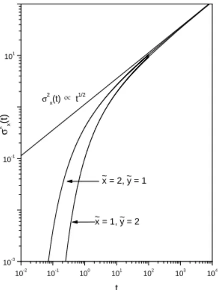
FIG. 1: Behavior ofσ2
xversustfor the initial conditionbρ(x,y) =
δ(x−ex)δ(y−ey)is illustrated for typical values ofexandey. Note that the spreading of the solution may exhibit an initial transient depend-ing on the choice of initial condition, i.e.,exandye, due to the structure of the system.
may also play an important role to investigate situations char-acterized by the system not initially localized at the point (x,y) = (0,0), for example, in drug deliver, flow transfer in disordered systems, tumor development or contaminant diffu-sion in a heterogeneous media. By using the above equation it is possible to find the dispersion relation forx andy di-rections which are useful to understand the diffusive process produced by the comb-model. By taking the initial condition ρ(x,y; 0) =δ(x−ex)δ(y−ey)into account, we can to show that the dispersion relation forx-direction is
σ2
x=2
D
xr t
π
D
ye− e y2
4Dyt +|ey|
D
xD
yerfc |ey| 2p
D
yt! (9)
and the dispersion relation for theyvariable isσ2
y =2
D
ytindicating that we have usual diffusive behavior in this direc-tion.
Now, we analyze Eq.(1) with
D
y(t) =D
ytγy−2/Γ(γy−1)(
D
y(s) =D
ys1−γyand 0<γy<1),D
x(t) =D
xtγx−2/Γ(γx−1)(
D
x(s) =D
xs1−γxand 0<γx<1), andµ=2. Notice that thischoice for the time dependence of the diffusion coefficients is related to the fractional time derivatives employed to analyze the subdiffusive processes. Other choices for the time depen-dence of diffusion coefficients are possible, however may lead us to a cumbersome calculations to obtain the inverse Laplace transform. For this case Eq. (1) can be written as
∂
∂tρ(x,y;t) = Z t
0
dt′
D
y(t−t′)∂2
∂y2ρ(x,y;t′) +δ(y)
Z t
0
dt′
D
x(t−t′)∂2
∂x2ρ(x,y;t′). (10)
with
D
y(t)andD
x(t)defined above. By taking the previousboundary and initial conditions into account one can show that the solution in the Laplace space is given by
ρ(x,y,s) =−
Z ∞
−∞dx
Z ∞
−∞dybρ(x,y)
e
G
(x,x,y,y,s) (11)with the Green function satisfying the equation
D
y(s)∂2
∂y2
G
e(x,x,y,y,s) +δ(y)D
x(s) ∂2∂x2
G
e(x,x,y,y,s)− s
G
e(x,x,y,y,s) =δ(y−y)δ(x−x) (12) and subjected to the conditionsG
(x,y,±∞,s) = 0 andG
(±∞,y,y,s) =0. After some calculations, the solution for above equation can be written as followse
G
(x,x,y,y;s) = − δ(x−x) 2psD
y(s)×
e− q s
Dy(s)|y−y|
−e− q s
Dy(s)(|y|−|y|)
− e
− r
2√sDy(s) Dx(s) |x−x|
q 8
D
x(s)p
s
D
y(s)e− q s
Dy(s)(|y|+|y|).
(13)
By using Eq.(11) and Eq.(13), one can find the dispersion relationsσx andσy in the Laplace space by considering the
initial conditionbρ(x,y) =δ(x−ex)δ(y−ey). Forσ2
x(s)we have
that
σ2x(s) =
D
x(s)p
s3
D
y(s)
e− q s
Dy(s)|ey|
(14)
and forσ2
y(s)we obtain thatσ2y(s) =2
D
y(s)/s2. Thesere-sults obtained forσ2
x(s)andσ2y(s)show that, depending on
the choice of
D
x(s)andD
y(s), the spreading of thedistribu-tion may exhibit different diffusive behaviors. By performing the inverse Laplace transform inσ2
x(s)andσ2y(s)and taking
the time dependence required above for the diffusion coeffi-cients into account we obtain that
σ2
x(t) =
D
xtγxp
D
ytγyH1,01,1 "
|y|
p
D
ytγy(
1+γx−γ2y, γy
2) (0,1)
#
σ2y(t) =
2
D
ytγyΓ(1+γy)
. (15)
Note that the dispersion relations obtained for this case in-dicate that the solution has an anomalous dispersion in both directions and depend on the parametersγxandγy. It is also
interesting to mention that the dispersion relation obtained for the y-direction is the same as the ones obtained for the fractional diffusion equations and the asymptotic behavior of σ2
x(t)istγx−γy/2for long time. In addition, the inverse Laplace
e
G
(x,x,y,y;t) = −pδ(x−x) 4πD
ytγyH1,01,1 "
(y−y)2
p
D
ytγy(
1−γ2y, γy
2) (0,1)
# −H1,01,1
"
(|y|+|y|)2
p
D
ytγy(
1−γ2y, γy
2) (0,1)
#!
−
Z t
0
dt (t−t)
r 8
D
xtγxq
D
ytγyH1,01,1 "s
2
D
xtγxq
D
ytγy|x−x|((β0,1,ξ))
# H1,01,1
|qy|+|y|
D
ytγy(
0,γ2y)
(0,1)
(16)
withβ=1−γx/2−γy/4 andξ=γx/2−γy/4.
Let us consider Eq.(1) with µ6=2. Applying the previ-ous procedure one can show that the solution is given by
ρ(x,y;t) =R−∞∞dxR−∞∞dybρ(x,y)
G
(x−x,y,y;t)with the Green function given byG
(x,y,y,t) = −pδ(x) 4πD
ytγyH1,01,1 "
(y−y)2
p
D
ytγy(
1−γ2y,γ2y)
(0,1) #
−H1,01,1 "
(|y|+|y|)2
p
D
ytγy(
1−γ2y,γ2y)
(0,1)
#!
− π1 |x|
Z t
0 dt (t−t)tγ2y
H2,12,3
2
q
D
ytγyD
xtγx |x|µ
(1,1),(β,ξ)
(1 2,
µ
2),(1,1),(1, µ 2)
H1,01,1
"
|y|+|y|
p
D
y(t−t)γy(
0,γ2y)
(0,1) #
(17)
withβ=1−γy/2 andξ=γx−γy/2.
3. DISCUSSION AND CONCLUSION
We worked out a non-Markovian Fokker-Planck by taking different scenarios into account, focusing on the comb-like structure. The solutions of this Fokker-Planck equation were obtained by considering the presence of time dependent dif-fusion coefficients, fractional spatial derivatives, and a gen-eral initial condition, which may be regarded as an interesting contribution in this context of comb-like structure. We start our analysis with the case characterized by the diffusion coef-ficients
D
y(t) =D
yδ(t)andD
x(t) =D
xδ(t)withµ=2. Thiscase is essentially the cases analyzed, for example, in Refs. [41, 42] for a particular initial condition. Here we consider a general initial condition for this case and show that if the sys-tem is not initially localized on the liney=0 the mean square displacement, variance, of the distribution inx-direction has an initially transient before recovering the subdiffusive be-havior characterized byt1/2. In addition, the solution has an addition term which is directly related to the choice of the
initial condition. Following, we incorporate a time depen-dence on the diffusion which may be related to time fractional derivatives. For this case, we also work out in the Laplace space - as general as possible - the solution and the variance inxandydirections. The results show that, depending on the choice of the diffusion coefficients, we may have different diffusive behaviors which remind us of the fractional diffu-sion equations of distributed order [48–50]. Afterwards, we considerµ6=2, i.e., we incorporate a spatial fractional time derivative onx-direction. The presence of this spatial frac-tional derivative on thexindicates that the solution in this di-rection is characterized by power law distribution which may be related to the L´evy distributions. For this case, as for the cases analyzed before, we obtain the exact solution. Finally, we expect that the results obtained here may be useful to in-vestigate systems where a comb- like structure is present.
ACKNOWLEDGMENTS
We thank CNPq/INCT-SC and Fundac¸˜ao Arauc´aria for par-tial financial support.
[1] A. Ott, J. P. Bouchaud, D. Langevin, and W. Urbach, Phys. Rev. Lett.65, 2201 (1990).
[2] H. Spohn, J. Phys. I France3, 69 (1993).
[3] T. H. Solomon, E. R. Weeks, and H. L. Swinney, Phys. Rev. Lett.71, 3975 (1993).
[4] F. Bardou, J. P. Bouchaud, O. Emile, A. Aspect, and C. Cohen-Tannoudji, Phys. Rev. Lett.72, 203 (1994).
[5] J. Stephenson, Physica A222, 234 (1995).
[6] A. Caspi, R. Granek, and M. Elbaum, Phys. Rev. Lett.85, 5655 (2000).
[7] Xiao-Lun Wu and A. Libchaber, Phys. Rev. Lett. 84, 3017 (2000).
[8] R. Hilfer, Applications of Fractional Calculus in Physics (World Scientific, Singapore, 2000).
[9] R. Metzler and J. Klafter, Phys. Rep.339, 1 (2000).
(2002).
[11] B. J. West, M. Bologna, and P. Grigolini,Physics of Fractal Operators(Springer, New York, 2002).
[12] G. M. Zaslavsky, Phys. Rep.371, 461 (2002).
[13] J. Klafter, M. F. Shlesinger, and G. Zumofen, Phys. Today49, 33 (1996).
[14] R. Hilfer, R. Metzler, A. Blumen and and J. Klafter,Strange Kinetics, Chemical Physics, 284 Numbers 1-2 (Pergamon-Elsevier, Amsterdam, 2004).
[15] R. Metzler, E. Barkai, and J. Klafter, Physica A 266, 343 (1999).
[16] D. Campos, V. M´endez, and J. Fort, Phys. Rev. E69, 031115 (2004).
[17] S. S. Plotkin and P. G. Wolynes, Phys. Rev. Lett.80, 5015 (1998).
[18] Y. E. Ryabov, Phys. Rev. E68, 030102 (2003).
[19] R. Metzler, E. Barkai, and J. Klafter, Europhys. Lett,46, 431 (1999).
[20] W. R. Schneider and W. Wyss, J. Math. Phys.30, 134 (1989). [21] F. Mainardi and G. Pagnini, Appl. Math. Comput. 141, 51
(2003).
[22] B. N. N. Achar and J. W. Hanneken, J. Mol. Liq. 114, 147 (2004).
[23] R. Gorenflo, A. Iskenderov and Y. Luchko, Fractional Calculus and Applied Analysis3, 75 (2000).
[24] Fu-Yao Ren, Jin-Rong Liang, wei-Yuan Qiu, Xiao-Tian Wang, Y. Xu, and R. R. Nigmatullin, Phys. Lett. A312, 187 (2003). [25] OM P. Agrawal, Nonlinear Dynamics29, 145 (2002). [26] A. Hanyga, Proc. R. Soc. London A458, 429 (2002). [27] S. A. El-Wakil and M. A. Zahran, Chaos Solitons & Fractals
12, 1929 (2001).
[28] S. A. El-Wakil, A. Elhanbaly, and M. A. Zahran, Chaos Soli-tons & Fractals12, 1035 (2001).
[29] E. K. Lenzi, R. S. Mendes, K. S. Fa, L. C. Malacarne, and L. R. da Silva, J. Math. Phys.44, 2179 (2003).
[30] E. K. Lenzi, R. S. Mendes, J. S. Andrade, L. R. da Silva, and
L. S. Lucena, Phys. Rev. E71, 052109 (2005).
[31] P. C. Assis da Silva, R. P. de Souza, P. C. da Silva, L. R. da Silva, L. S. Lucena, and E. K. Lenzi , Phys. Rev. E73, 032101 (2006).
[32] K. Seki, M. Wojcik, and M. Tachiya, J. Chem. Phys.119, 2165 (2003).
[33] S. B. Yuste, L. Acedo, and K. Lindenberg, Phys. Rev. E69, 036126 (2004).
[34] I. M. Sokolov, M. G. W. Schmidt, and F. Sagu´es, Phys. Rev. E
73, 031102 (2006).
[35] R. Rossato, M. K. Lenzi, L. R. Evangelista and E. K. Lenzi, Phys. Rev. E76, 032102 (2007).
[36] L. S. Lucena, L. R. da Silva, L. R. Evangelista, M. K. Lenzi, R. Rossato, and E. K. Lenzi, Chem. Phys.344, 90 (2008). [37] V. E. Arkhincheev, JETP Letters86, 508 (2007).
[38] I. A. Lubashevski and A. A. Zemlyanov, JETP87, 700 (1998). [39] V. E. Arkhincheev, JETP88, 710 (1999).
[40] A. M. Reynolds, Physica A334, 39 (2004). [41] V. E. Arkhincheev, Physica A280, 304 (2000). [42] V. E. Arkhincheev, Chaos17, 043102 (2007). [43] K. V. Chukbar, JETP82, 719 (1996). [44] A. Iomin, J. Phys.: Conf. Ser.7, 57 (2005).
[45] I. Podlubny, Fractional Differential Equations (Academic Press, San Diego, 1999).
[46] M. P. Morse and H. Feshbach,Methods of Theoretical Physics (McGrawHill, New York, 1953).
[47] A. M. Mathai and R. K. Saxena,The H-function with Appli-cation in Statistics and other Disciplines(Wiley Eastern, New Delhi, 1978).
[48] A. V. Chechkin, R. Gorenflo, and I. M. Sokolov, Phys. Rev. E
66, 046129 (2002).
[49] I. M. Sokolov, A. V. Chechkin, and J. Klafter, Acta Phys. Pol. B35, 1323 (2004)