J. Microw. Optoelectron. Electromagn. Appl. vol.10 número1

Abstract_{— This paper presents the results of measurements and}

simulations of the characteristics of 900 MHz band radio propagation channels in a tunnel environment. The simulations were made using the FDTD method (with companion UPML) and measurements made use of the swept frequency technique. Another method, the metaheuristic Simulated Annealing, was implemented for estimating the values of characteristic parameters of materials. The FDTD code was reformulated for use with CUDA with the objective of decreasing program running time.

Index Terms—Tunnel, CUDA, FDTD, Simulated Annealing.

I. INTRODUCTION

A special type of indoor environment, tunnels are relevant for systems serving both roads and

railways as well as in urban subway services. Leaky feed cables have been customarily used inside

tunnels with the communication being provided by stringing wires over the length of the tunnel or by

placing repeaters at intervals, or both. These methods are expensive to install and inconvenient, need

regular maintenance, could be unreliable in disaster situations and do not allow an in-tunnel mobile

user to transmit. The use of discrete antennas inside tunnels can avoid the above shortcomings, with

the possible advantage of needing no prior infra-structure in peer-to-peer wireless communications.

The Finite-Difference Time-Domain (FDTD) method [1] is implemented with companion of

Uniaxial Perfect Matched Layers (UPML) [2] to access the power delay profile and channel related

parameters of a subway tunnel in Hong Kong, China, for a wide band UHF range centered at 900

MHz [3], [4]. Simulated results are compared with measurement data, validating the channel

characterization. Equipment comprised a network analyzer, a sweep oscillator and discone antennas

for both the transmitter and receiver ends as described in Section IV, while modelling techniques and

the implementation of simulation are reviewed in section II and III, respectively.

II. MODELLING

A. Scenario modelling

The scenario in Fig. 1.a, corresponding to the second of three sections of a Hong Kong subway

tunnel, has a rectangular cross section with height and width 3.43 m and 2.6 m, respectively, central

Channel Characteristics in Tunnels:

FDTD Simulations and Measurement

L.A.R. Ramirez, F.J.V. Hasselmann,

CETUC - Centro de Estudos em Telecomunicações – Pontifícia Universidade Católica do Rio de Janeiro Rua Marquês de São Vicente, 225, 22451-900, Rio de Janeiro, RJ, Brazil,

{luis, flavio}@cetuc.puc-rio.br

Y.P. Zhang

section 107.7m long, walls in reinforced concrete (relative permittivity εr=3.28 and conductivity σ=

0.05 S/m, approximate values calculated according to the technique in B), with antenna positions

depicted in Fig.1.b

Fig. 1. Hong Kong subway tunnel (a) photo (b) structure used in the simulation.

B. Simulated Annealing Technique: Practical Implementation for Characteristic Parameters Estimation.

Lack of knowledge of characteristic parameters of walls materials made it necessary the use of a

meta-heuristic technique, called "simulated annealing", in order to minimize the difference between

estimated and measured values.The concept of the method is based on the manner in which liquids

freeze or metals recrystalize in the process of annealing, thereby transforming a poor, unordered

solution into a highly optimized, desirable one [5][6]. This process of reducing the mismatch is called

calibration and it consists in extracting relevant multipath components (MPCs), for instance once

reflected paths, simultaneously from the model and measurement. Afterwards, the simulated

annealing is performed to optimize the material parameters. The calibration was performed using the

measurements for LOS case Tx-Rx1 in Fig.1. Fig. 3 displays the obtained (before and after

calibration) and measured power delay profile (PDP). As expected, the calibrated PDP shows a better

match with the measured PDP for Tx-Rx1. The values encountered were used for the other cases

considered in this work.

Details of the implementation are described in the following paragraphs. In the process of

annealing used, the initial material properties were defined using known tabulated values for

reinforced concrete (εr= 4.95 and conductivity σ= 0.01 S/m) available in the literature[7].

As the relation between the power taps and material parameters is a non linear combinatorial

relationship, this technique provides the general optimal solution by simultaneously changing the

dielectric constant and conductivity of concrete parameters with a changing step at each range of

iterations, for relevant multipath components(MPC).

The algorithm considers a subset of M measurements with Pi power taps from each measurement i.

The objective function, defined as the root mean square error (RMSE) between the measured and the

or value of the present minimum, computed at each iteration k = i.j as

( )

( )

1 1

1

1

k ij _pred ij _meas k i i j

RMSE

a

a

M

P





=

_

−

_





∑

∑

where the parameters

(

a

)

(

a

)

MPC from the i-th measurement.

In the SA algorithm, random steps in the parameter space are performed using a control parameter

T which is decremented as the algorithm progresses. A step is always accepted if the objective

function is lowered, and it is sometimes accepted with a certain, decreasing probability, if an uphill

step is taken. Its decreasing probability exp[−∆RMSE/T ] is a function of the variables (RMSEi ,

RMSEi-1 and T ), where ∆RMSE is the difference between the actual RMSEi and its neighbor RMSEi-1.

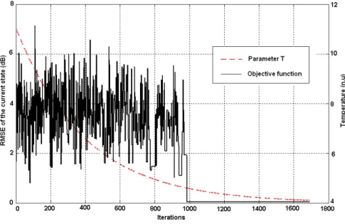
This scheme allows the algorithm to escape from local minima. By decreasing the step, it computes

the best value at each iteration as depicted in Fig. 2 with 1764 iterations for the convergence of the

simulated annealing algorithm when minimizing RMSE. The objective function evolves from 7 dB to

an optimal value of 0.3 dB for which the material parameters of the database are changed.

Fig. 2. Evolution of the RMSE of the FDTD prediction when choosing the material parameters using simulated annealing for an objective function variation within 42x42 iterations. The parameter T is expressed in natural units.

The algorithm stops after a certain number of steps NS if there is no significant change in the

objective function. After termination, the final configuration is taken as the solution and a file

containing the optimized parameters is produced. This optimized parameters can then be used by the

Fig. 3. Power delay profile comparison (measurement, uncalibrated and calibrated method).

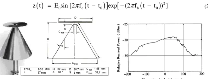
C. Antenna modelling

The transmitter (Tx) and receiver antennas (Rx1, Rx2) in Fig. 1 are discones fabricated for the 900

MHz band, operating along wide bandwidths (>400 MHz). The Tx antenna, shown in Fig. 4.a, was

inserted in the FDTD grid and components of electric field tangential to (metallic) elements

considered null, with excitation as in (2).

The generated driving signal in (2) has a central frequency (fc) of 900 MHz over a band (fb) of 450

MHz and t0=5 ns denotes the initial delay; signal (normalized) amplitude and its frequency contents

are illustrated in Figs. 5.

( )

(

)

]

[

(

)

0 c 0 b 0

z t

=

E sin [2 f

π

t

−

t

exp

−

(2 f

π

t

−

t ) ]

Fig.4.(a) Dimensions of transmitter and receiver antennas for 900 MHz. (b) Measured horizontal plane radiation pattern of discone antennas at 900 MHz.

Fig. 4.(b) illustrates their measured co-polarized horizontal plane radiation patterns at 900 MHz.

III. FDTDIMPLEMENTATION

As for the implementation of the FDTD method for the most critical configuration, the

which, for a working frequency of 900 MHz (wavelength λ=0.3331 m), corresponds to ∆x = 0.0333

m. Numerical dispersion was thereby avoided and, by proper choice of the temporal step (∆t = 0.0577

ns), calculated according to Courant criteria [1] and used in central difference approximation of

Maxwell equations, numerical stability was assured. Also, for the truncation of the domain, 7 UPML

layers were implemented accordingly [2].

Fig.5. Pulse excitation of Tx antenna and its frequency spectrum.

A. CPU implementation

For the scenario (60.0 x 3.43 x 2.6 m) scenario at hand and a spatial step of 0.0333 m, a total of

16251 FDTD cells are represented, each cell associated to six (electric and magnetic) field values as

well as to six flags indicative of the type of material present at each spot. Also, field values are 4 bytes

real numbers while flag lengths are 1 byte each, implying a memory need of 30 bytes per cell and a

total memory requirement of circa 8.366 GBytes to address the present problem, which was perfectly

handled by available 24 GBytes (RAM) processors. With the time step used, however, 17321x106

iterations were necessary to address the 500 ns duration of the simulations displayed above, rendering

approximately 5 hours of computer time. In order to remedy this problem, the original code in C

language was translated to CUDA (Compute Unified Device Architecture), a parallel computing

architecture that use C with Nvidia extensions[8].

B. GPU implementation

Recent developments in graphics hardware acceleration provide operations that can be applied to

dramatically speed up FDTD simulations and the economy of scale gained by 3D graphics cards due

to the burgeoning video-game/entertainment industry provides a considerable cost/performance

advantage. Graphics processing units (GPUs) are very fast, very cheap, and continue to be enriched at

rates that outstrip those of general purpose CPUs. GPUs are constructed in a superscalar fashion. A

GPU is implemented as an aggregation of multiple so-called multiprocessors, which consist of a

number of SIMD ALUs (Single Instruction Multiple Data Arithmetic Logic Unit). A single ALU is

called processor. According to the SIMD concept, every processor within a multiprocessor must

execute the same instruction at the same time, only the data may vary[9]. The software model of

GPUs for parallel computation with minimum graphics knowledge, the framework CUDA providing

to the programmer a minimal extension to use functions named kernel to call a process a number of

times concurrently. In the CUDA model, being each data processed by an individual thread, each

thread runs a distinct process or program. Threads are organized inside blocks, and blocks are in turn

grouped inside grids. The kernel is called using a global declaration and the number of threads and

blocks. Each process runs on a thread, and each thread has a number for its identification[8]. Each

multiprocessor has a small shared memory that can be accessed from each of its processors, and there

is a large global memory space common to all the multiprocessors. Shared memory is very fast and is

usually used for caching data from global memory. Both shared and global memory can be accessed

by any thread for reading and writing operations without restrictions[8].

These multiple levels of memory hierarchy are quite different from the common CPU

memory/cache model. The CUDA memory hierarchy is composed of a large on-board global memory

which is used as main storage for the computational data and for synchronization with the host

memory. Unfortunately, the global memory is very slow and not automatically cached. To fully utilize

the available memory bandwidth between the global memory and the GPU cores, data has to be

accessed consecutively. To alleviate the high latencies of the global memory, a shared memory can be

used. Shared memory is explicitly managed by the kernel and special care has to be taken when it is

accessed. When the same shared memory banks are accessed by multiple threads at the same time, a

memory access conflicts will occur and the readings to the same memory bank will be serialized[9].

A general-purpose computing on GPUs so-called GPGPU applications follows the steps:

1. Define and reserve memory for CPU and GPU data structures. 2. Copy data from CPU to GPU global memory

3. Define numThreads and numBlocks variables 4. Execute CUDA procedure for each thread 5. Copy data results from GPU to CPU 6. Free GPU data structures

The initial CUDA FDTD version of the code was implemented to work on GPU Quadro FX 1800

series with clock rate: 1400 MHz, multiprocessors: 8, threads per block: 512, global memory: 767.688

MB, memory shared per block: 16 KB. The (x,y,z) E and H field components were stored on the

device memory as 32 bit floating point variables. A texture memory was used to store, as a pointer

stream, the material types in the model space. In both of these cases, the 3D volume was flattened into

2D and was accessed via an algorithm based on 3D to 2D address translation. This allows the entire

3D space to be updated in one render pass and also avoids potential "read after write" data corruption.

The material type pointer stream was used for material property lookups stored in textures. E and H

scattered field update calculations were converted to fragment programs, taking the E and H fields

values stored in textures as inputs. Between each time step, input and output memories on the device

are swapped providing a feedback loop and avoiding the performance penalty of pushing data across

to the CPU version one, it is believed that this should improve in upcoming versions of the program

due to ongoing code optimization processes.

IV. MEASUREMENTS

The wideband experimental setup is shown in Fig. 6 [3], [4]. The system consists of an HP 8350B

sweep oscillator, 8510C network analyzer, and 8517A -parameter test set. Port 1 was connected to the

transmit antenna through a 10-m coaxial cable. The power outputted to the transmit antenna was 15

dBm. The transmitted sweep frequency waves were captured by the receive antenna connected to port

2 through another 50-m cable. The measured data of wideband propagation characteristics was stored

onto a floppy disk of the network analyzer for subsequent analysis.

Fig. 6. The wideband experiment setup.

V. COMPARASION BETWEEN SIMULATED AND MEASURED DATA

Three situations were considered. In the line-of-sight (LOS) one (Figure 1), Rx1 was located very

near (5m) Tx and Rx2 was placed in the middle of the tunnel (antennas 50m apart). In the NLOS

situations, the receiver antenna Rx3 was separated 20m from the transmitter one and the path was

obstructed by a vehicle modelled by a perfectly conducting parallelepiped of dimensions 1.0m x

1.35m x 0.45m placed above the ground and located 10m away from Tx.

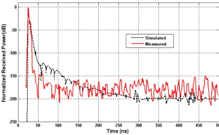
Fig. 7. Simulated (dashed line) and measured (continuous line) averaged 900 MHz vertically polarized power delay profile (LOS). The distance between antennas is 5 m.

polarized power delay profiles for a 5 m antenna separation. The first signal to reach the receiver,

along the direct ray, is depicted at about 26ns, with previous contributions corresponding to noise.

Deviations between measurement and simulations, thereafter, are credited to probe resolution which

fails to take into account relevant reflected ray contributions for short distances between transmitter

and receiver antennas.

Figure 8 show the comparison between averaged 900 MHz vertically polarized power delay profiles

for a 50 m antenna separation, which permits the probe resolutions to yield measured data followed

more closely by simulations. Also, as expected, the main contribution following a direct propagation

path, detected at about 167 ns, is observed to be substantially stronger than those reaching the receiver

via reflected paths with partial energy carried by the delayed waves being inevitably absorbed by the

tunnel walls.

Fig. 8. Simulated (dashed line) and measured (continuous line) averaged 900 MHz vertically polarized power delay profile (LOS) The distance between antennas is 50 m.

Fig. 9. Simulated (dashed line) and measured (continuous line) averaged 900 MHz vertically polarized power delay profile (NLOS). The distance between antennas is 20 m with the path obstructed by a vehicle located 10m away from the transmitter

antenna.

profile for a 20 m antenna separation with the line-of-sight path obstructed by a vehicle located 10 m

away from the transmitter antenna. The direct signal reaches the receiver at 52 ns while the delayed

(reflected) ones become stronger thereon, recovering maximum (line-of-sight) field intensity at 76 ns.

At about 200 ns, scattering by the vehicle is observed to play its role. Again, equipment resolution is

due to account for occasional deviations between interference curves.

VI. CONCLUSION

In this work, a comparasion between (FDTD) simulated and measured results for the averaged

power delay profile along a subway tunnel of simple cross section and finite conductivity walls, for

both empty and partially filled situations, was presented. Although a good agreement between results

has been observed, two important aspects of the simulations were revealed and explored. The

determination of characteristic parameters of materials from the knowledge of measured data was

addressed by the simulated annealing technique, which may yet be generalized and its implementation

optimized. Also, excessive computing times, typical of this category of numerical simulations, were

shown to be alleviated via the CUDA parallel programming route and further investigation and

implementations are likely to improve its efficiency.

Work in progress explores the application of the techniques employed herein to tunnels of more

general cross sections and more complex fillings, aiming at fully understanding the propagation of

radiowaves in tunnels.

Future work will address the analytical description of mode guiding in tunnels in order to

investigate coverage characteristics along extended frequency bands. Modal analyses can then be

converted into ray-optical ones via appropriated Poisson Sums to access the localized tracking of field

contributions to specific observation regions and, through Fourier inversions, the corresponding

evolutions in time. In this way, a physical transparency may be added to FDTD results such as these

presented herein, therefore contributing to its interpretation and desired validation. Once this is

achieved, one gains confidence in exploring the implementation of FDTD to simulate the EM

coverage of more complex and arbitrary tunnel scenarios, whereby frequency-domain analytical

efforts tend to be cumbersome and diversified for broad band purposes.

REFERENCES

[1] A. Taflove, and S. C. Hagness, “Computational Electrodynamic: the Finite-Difference Time-Domain Method”, 3rd Edition., Arthec House Publishers, 2005.

[2] S. D. Gedney, “An anisotropic perfectly-matched layer-absorbing medium for the truncation of FD-TD lattices,” IEEE Transaction Antennas Propagation., vol. 44, pp. 1630–1639, Dec. 1996.

[3] Y.P. Zhang, Y. Hwang and P.C. Ching "Wide-Band UHF Radio propagation Characteristics in a Tunnel Environment", Wireless Personal Communications 8: 291-299, 1998.

[4] Y. P. Zhang, Y. Hwang, “Characterization of UHF radio propagation channels in tunnel environments for microcellular and personal communications” IEEE Trans. on Vehicular Technology, Vol. 47, No. 1, pp.283-296, February 1998.

[5] S. Kirkpatrick, C. D. Gelatt, M. P. Vecchi (1983-05-13). "Optimization by Simulated Annealing". May 1993. Science. New Series 220 (4598): 671–680

[7] H. C. Rhim and O. Buyukozturk, “Electromagnetic properties of concrete at microwave frequency range,” ACI Materials Journal, vol. 95, no. 3, pp. 262–271, 1998.

[8] NVIDIA CUDA (Compute Unified Device Architecture): Programming Guide, Version 3.0. Feb 2010 http://developer.download.nvidia.com/ compute/cuda/3_0/docs/.

[9] T. Rauber and G. Runger, Parallel Programming for multicore and cluster system, Springer-Verlag , 2010.

ACKNOWLEDGEMENT