UNIVERSIDADE DO ALGARVE
UNIVERSITY OF ALGARVE
FACULDADE DE CIÊNCIAS E TECNOLOGIA
FACULTY OF SCIENCES AND TECHNOLOGY
“Assessment of Sea Surface Temperatures (SST)
and Seasonal upwelling in SW Portugal”
MESTRADO EM GESTÃO DA ÁGUA E DA COSTA
(CURSO EUROPEU)
ERASMUS MUNDUS EUROPEAN JOINT MASTER
IN WATER AND COASTAL MANAGEMENT
(BY: NDUI AIKAYO)
FARO 2010
NOME / NAME:
Aikayo, Ndui
DEPARTAMENTO / DEPARTMENT: Química, Bioquímica e Farmácia
– Faculdade de Ciências e Tecnologia da Universidade do Algarve
ORIENTADOR /SUPERVISOR:
Professor Alice Newton
Co Supervisor: Dr. John Icely
University of Algarve Faculty of Science and Technology (FCT)
DATA / DATE: 15-03-10
TÍTULO DA TESE / TITLE OF THESIS:
Assessment of Sea Surface Temperatures (SST) and Seasonal
upwelling in SW Portugal.
JURI:
Prof. Tomasz Boski
Dr. John David Icely
Dr. Flávio Augusto Bastos da Cruz Martins
Prof. Alice Newton
Dr. Emilie Brévière
ACKNOWLEDGEMENTS
I express my acknowledgements to the Erasmus Mundus External window cooperation
-Lot 10 Programme awarded by European Commission for funding the European Joint
Master in Water and Coastal Management and this research.
I would like to thank my supervisors, Professor Alice Newton and Dr.John Icely
(University of Algarve, Portugal) for their continuous assistance, comments, suggestions
and guidance’s throughout my study.
My Special thanks to the Government of the Republic of Zambia (GRZ) through the
Ministry of Communications and Transport (MCT) at the Zambian Meteorological
Department (ZMD), for granting me study leady to come and study this very important
Master.
I extend my sincere thanks to Dr. Simon Mason of International Research Institute (IRI),
for his technical assistance on the CPT software, Damian Icely on the Ferret software,
MR. Faqih Akhmad of Center for Climate Risk and Opportunity Management in
Southeast Asia and Pacific (CCROM-SEAP),and Department of Geophysics and
Meteorology, Bogor Agriculture University ,Indonesia for installing a Microsoft version
of Ferret on my Laptop, Bruno Fragoso and Sonia Cristina for their assistance on Data
analysis, and sites.
I would like to thank all my friends for their love and help during my study and project
work in Europe. Finally I would like to thank my parents, family and all those who have
extended their help to me.
iii
Resumo
Informação meteorológica como a Temperatura de Superfície do Mar (SST), a Direcção e
Velocidade do vento, são parâmetros importantes para determinar a ocorrência de
afloramento costeiro. Neste estudo são apresentadas técnicas, que podem ser usadas para
determinar dados meteorológicos em falta nas bases de dados, nomeadamente das
autoridades meteorológicas nacionais. O programa Climate Predictability Tool (CPT) foi
usado para determinar os valores em falta nas séries de dados através da Regressão de
Componentes Principais (PCR). Para calcular as relações entre as séries de dados foi
usado o SYSTAT e os gráficos derivados do FERRET gerados a partir das imagens de
satélite. Os resultados indicam que os valores do arquivo do
www.windguru.cz
para
Sagres (SW Portugal), são mais adequados para substituir valores em falta de
temperatura, mostrando uma relação na ordem do 88% relativamente aos dados in situ.
Por outro lado, os gráficos gerados pelo FERRET indicam que podem ser alternativa para
gerar os dados de direcção e velocidade do vento.
Em geral, o afloramento costeiro envolve processos físicos, químicos e biológicos. Em
relação aos processos físicos, a água fria oriunda do fundo determina a temperatura da
superfície do mar. O vento representa um papel importante na regulação da temperatura
da superfície do mar e transporte do calor do oceano. A nível químico, o transporte de
águas ricas em nutrientes do fundo até á superfície, promove os processos biológicos,
como a ocorrência de florescências de fitoplâncton resultando num aumento de clorofila
causando a alteração da côr da água, que pode ser detectada através de imagens de
satélite.
Informação disponível no sítio de internet do Windguru e os gráficos do FERRET podem
ser adequados para completar dados em falta das bases de dados.
Informação adicional, sobre condições meteorológicas e oceanográficas que são
responsáveis pela ocorrência do afloramento costeiro, estão disponíveis neste trabalho.
Palavras-chave:
Afloramento costeiro, Temperatura das Superfície do Mar (SST), Vento, FERRET,
SYSTAT, Windguru
ABSTRACT
Meteorological data such as Sea Surface Temperature (SST), Wind direction and Wind
speed are important parameters to determine the occurrence of upwelling. This study
demonstrates some useful techniques that can be used to provide useful meteorological
data, where these may be missing from conventional data sets that are provided by, for
example, national meteorological authorities. The techniques used include: Plotting the
daily temperature datasets in Lines on 2Axes using EXCEL,the nearest neighbour station
using Principal Component Regression in Climate Predictability Tool (CPT), calculating
the skills by comparing the two datasets using SYSTAT and using FERRET satellite
derived data plots to determine the missing data for a particular time. Results showed that
the www.windguru.cz dataset for Sagres (SW Portugal) proved to be more suitable for
replacing the missing data of temperature on the Meteorological datasets because the
skills were as high as 88%, comparing with in situ data. FERRET plots also indicated
suitable substitutes for non availability of the Meteorological data such as wind direction
and speed.
In global scenario, upwelling involves the Physical, Chemical and Biological process.
Physically-like cold water on the surface because of upwelling and this affects Sea
surface temperature. Wind plays an important role in regulating the Sea Surface
Temperature (SST) transporting heat through the surface water. Chemically - nutrients
rich water brought to the surface and Biologically-production of phytoplankton bloom
that results into chlorophyll increase and this gives the resulting color change in ocean
color which can be detected by satellite images.
Data from the Windguru website archive and the Ferret derived plots are suitable for
replacing where they are missing data on the Meteorological datasets.
Details and a short review of the oceanographic and meteorological conditions that are
responsible for upwelling are presented in the text.
Keywords:
Upwelling, Sea Surface Temperatures (SST), Wind, FERRET, SYSTAT, Windguru
v
LIST OF ABBREVATIONS
AIRT Air temperature
AOU Apparent Oxygen Utilization
AVHRR Very high resolution radiometer
AWS Automatic weather station
CAS Central American Seaway
CPT Climate Predictability Tool
CZCS Coastal Zone Color Scanner
DLESE Digital Library for Earth System Education
ENSO El Niño Southern Oscillation
GUI Graphical user interface
HAB Harmful Algal Bloom
ITCZ Inter Tropical Convergence Zone
IRI International Research institute for Climate and
Society.
MGSVA Mariano Global Surface Velocity Analysis
NOAA National Oceanic and Atmospheric Administration
NAO North Atlantic Oscillation
NAOI Northern Atlantic Oscillation Index
NASA National Aeronautics and Space Administration
NCOF National Center for Oceanic Forecasting
PC The Portugal Current
PC Peruvian Current
PCC The Portugal Coastal Current
PCCC The Portugal Coastal Countercurrent
PCR Principal Components Regression
PMEL Precision Measurement Equipment Laboratory
SAA South Atlantic Anticyclone
SLP Sea Level Pressure
SPEH Specific humidity
SOI Southern Oscillation (ENSO) Index
SSH Sea Surface Height
SST The Sea Surface Temperature
STN Station
THC Thermohaline circulation
TMAP Thermal Modeling and Analysis Project
UWND Zonal wind
VWND Meridional wind
WHWP Western Hemisphere Warm Pool
WSPD Wind speed
WX Weather
TABLE OF CONTENTS
S. NO
PARTICULARS
PAGE NO
1 Introduction
1
2 Study
Area
1
2.1
Coast of SW Portugal (Sagres)
2
2.2
Upwelling along Sagres coast ( SW Portugal
5
3
Objective of the study
8
4 Research
questions
9
5
Materials and Methodology
9
5.1
Data Management and description
9
5.2 First Approach
10
5.3 Second
Approach
11
5.4 Third
Approach
12
6 Results
and
Discussion
14
7 Conclusions
29
8 References
30
Appendix A- Review
32
1 Review
32
2
Global Climate-Coupled Ocean-atmospheric
34
2.1
El Niño Southern Oscillation(ENSO)
34
2.1.1.
El Niño Sotuer Oscillation(ENSO)Index
35
2.1.2 El
Nińo 35
2.1.3 La
Nińa 36
3
Ocean winds and Circulation
36
3.1
Ocean Surface Circulation
37
4
Northern Atlantic Winds
38
4.1
Northern Atlantic Oscillation(NAO)
38
4.2
Northern Atlantic Oscillation Index
39
5 Upwelling
40
5.1 Downwelling
41
5.2
Mechanisms that Cause Ocean Upwelling
41
5.2.1
Physical application of Upwelling
42
5.3
The Coriolis Effect
42
5.3.1 Climatic
rainfall
43
5.4
Types of Upwelling
43
5.4.1
Coastal upwelling
43
5.4.2 Equatorial
upwelling
44
5.4.3 Seasonal
upwelling
44
5.5
Sea Surface Temperatures (SSTs)
45
5.5.1
Identifying Upwelling on Satellite-derived Maps
45
5.6 Remote
sensing
46
5.7
Biological effect on upwelling
46
5.8 Chlorophyll
47
6 References
52
Appendix B-
Figures for Review
55
Appendix C-
Tables
72
LIST OF FIGURES IN THE STUDY
1
Maps showing the general and specific location of Sagres
2
2
The Portugal Current System
3
3
Coastal upwelling along the Sagres coastline
6
4
Missing Values in CPT
11
5 Principal
Components
Regression in CPT.
12
6
Plot of temperatures for August 2009
15
7
Plot of Skills between the temperature datasets for Aug.2009
16
8
Plot of temperatures for September 2009
16
9
Plot of Skills between the temperature datasets for Sept.2009
17
10
Plot of temperatures for October 2009
17
11
Plot of Skills between the temperature datasets for Oct.2009
18
12
Wind direction and Speed for August to October 2009
19
13
Wind direction and Speed for 1999
19
14
Example of Ferret Sea Surface Temperatures
20
15
Example of Ferret winds
20
16
Example of Ferret Air Temperatures
21
17
Ferret surfsce Winds for 20
thAugust 1999,in vector formart
22
18
Ferret surfsce Winds for 20
thAugust 1999
24
19
Ferret surfsce Winds for 19
thAugust 1999
25
20
Ferret surfsce Winds for 21
stAugust 1999
25
21
August 1999 Sagres daily Temperatures
26
22
Ferret surface Winds for 20
thAugust 1999,in vector format
overlaid on number of observations(count)
26
23
Ferret surface Winds for 19
thAugust 1999,in vector formart
overlaid on number of observations(count
)27
24
Ferret surface Winds for 21st August 1999,in vector formart overlaid onnumber of observations(count)
28
25
August 1999 temperature logger daily sea Temperatures28
LIST OF FIGURES FOR REVIEW
Figure N0. Page
1
General Areas of upwelling
55
2
Warm and cold water current
55
3
El Nino-Southern Oscillation event
56
4 ENSO-Neutral
conditions
56
5
The Southern Oscillation Index (SOI)
56
6
IRI Probabilistic ENSO Forecast for NINO 3.4 Region
57
7
El Niño and La Niña conditions
57
8 The
general
circulation
58
9
Wind effect on surface water currents
58
10
The trade winds are part of the Earth's atmospheric circulation
59
11
Atlantic Ocean circulation
59
12 Satellite
sea-surface
temperature image of the Gulf Stream
60
13
Near surface circulation of the North Atlantic Ocean
60
14
The NAO index
61
15
The North Atlantic Oscillation Index61
16
The Trade winds and strong equatorial currents
61
17
Upwelling and Downwelling Areas
62
18
Causes of upwelling
62
19
The Coriolis force
62
20
Cold water being upwelled to the surface
63
21
Sea surface temperatures during upwelling period
64
22a
Upwelling near the coast due to Ekman transport
64
22b
The Ekman spiral (southern hemisphere
)65
23
Annual rainfall
65
23a
Showing the upwelling affecting Deserts
66
23b
Namibian upwelling –Kalahari Desert
66
24 Coastal
Upwelling
67
25 Equatorial
Upwelling
67
26 Seasonal
Upwelling
68
27
Latest global sea surface temperature and sea ice analysis
68
28
The deep water that surfaces in upwelling is cold
69
29
Signal and data flow in a remote control system
69
30 Phytoplankton
photosynthesize using chlorophyll
70
31 Marine
ecosystem
70
32 Primary
Production
image
71
33
Ocean chlorophyll concentration off the coast of Sagres
71
LIST OF TABLES –Appendix C.
1
April mean temperature with missing values and satellite grid data
72
2
Replaced missing April data
73
3
August 2009 Temperature for Computer generated Sagres weather station and Windguru
data.
73
4
Table 4. September 2009 Temperature for Computer generated Sagres weather station and
Windguru data.
74
5
Table 5. October 2009 Temperature for Computer generated Sagres weather station and
Windguru data.
75
6
Showing the seven variables in 2˚x2˚,for global for Ferret
75
7
Showing windguru speed and direction for three months of August to October 2009
76
8
Showing August 1999 wind direction and Speed for Sagres.
78
9
IRI Probabilistic ENSO Forecast for NINO3.4 Region - Made in September 2009.
78
10 August 1999 daily sea temperatures
79
Xi
1. INTRODUCTION
Coastal upwelling is a phenomenon, with dramatic effects on physical, chemical and biological processes (Sousa and Bricaud, 1992; Conway, 1997; Wollast, 1998; Harimoto et al., 1999; Brogueira et al., 2004; Loureiro et al., 2005; Relvas et al., 2007; Loureiro et al., 2008). A short review of the oceanographic and meteorological conditions that are responsible for upwelling events is provided in Appendix A. Considering the profound influence of upwelling events on biological processes in the locations where they occur, it is important to have good information about meteorological and oceanographic conditions in order to understand the chemical and biological processes that occur before, during and after upwelling events. Many scientists working on these processes depend on other authorities to provide them with background information on meteorological and even oceanographic conditions. However, there are many situations where this data is incomplete. The objective of this study is to demonstrate some techniques that can be used to provide useful meteorological data, where these may be missing from conventional data sets that are provided by, for example, national meteorological authorities. This study will be based on actual data sets collected historically and recently from Sagres in an upwelling area on the SW coast of the Iberian peninsular.
2. Study Area
Sagres is on the south west coast of Portugal, located at 37°N and 8.95°W, it is located at the extreme south-west of Algarve. (Fig.1.below). Climate of the area can be divided into two; the southern Sagres has Mediterranean type which is warmer and the western part which is colder, stormy and is exposed to waves.
Iberian Peninsula (Fig. 1) is affected by seasonal upwelling induced by northerly winds from May to September (Wooster et al., 1976; Fiúza, 1983; Sousa and Bricaud, 1992).
Fig.1. Maps showing the general and specific location of Sagres (Adapted from: Fragoso and Icely, 2009).
2.1. Coast of SW Portugal (Sagres)
The Portugal Current (PC) system, defines the classic strictly southerly flow regime as typically depicted in marine atlases and pilot charts, when observed at yearly time scales. The entire system extends from about 36°N to about 46°N and from the Iberian shores to about 24°W (Perez et al., 2001; Martins et al., 2002). The Portugal Current itself is poorly defined spatially because of the intricate interactions between coastal and offshore currents, bottom topography, and water masses. The system is comprised of the following main currents: 1) The Portugal Current, which is a broad, slow, generally southward-flowing current that extends from about 10°W to about 24°W longitude; 2) The Portugal Coastal Countercurrent (PCCC), a southward flowing surface current along the coast during downwelling season, mainly over the narrow continental shelf to about 10-11°W longitude and flow from about 41-44°N; and 3) the Portugal Coastal Current (PCC), a generally poleward current that dominates over the PCCC during times of upwelling and like the PCCC, extends to about 10-11°W from
shore, also present mainly from 41-44°N, where flow is 13.5 ± 5.7 cm s-1 (Perez et al., 2001; Martins et al., 2002). Fig. 2 shows the Portugal current system in three monthly seasonal averages. The Portugal current as represented by the Mariano Global Surface Velocity Analysis (MGSVA). The average flow is towards the south and feeds the Canary Current. Highlighted in red in the figures is the area where the coastal current can flow northward, depending on the winds The Portugal currents, has the mean pattern as well as seasonal variation and are well established despite relatively few systematic observations. The Portugal and Canary Currents form the eastern limb of the North Atlantic Subtropical Gyre (Barton, 2001).
(B) Apr-May-Jun
(D) Oct-Nov-Dec
Fig.2. The Portugal Current System from January to December, From: Bischof et al., 2003) http://oceancurrents.rsmas.miami.edu/atlantic/portugal.html.
2.2. Upwelling along Sagres coast ( SW Portugal
Upwelling takes place along the Sagres coast of Portugal during the summer under the fairly strong and steady northerly winds. Studies of Upwelling in the Portuguese coastline have been done and papers have been published on the same topic by authors such as ( Santos et al., 2001; Relvas and Barton, 2002; Loureiro et al., 2008; Fragoso and Icely, 2009). Others are (Villa et al., 1997; Peliz et al., 2001; Loureiro et al., 2005 ). Upwelling responds quickly to northerly winds, particularly south of capes, appearing first along the coastline and then spreading offshore as the event progresses (Fiúza et
al., 1982).The Portugal Coastal Current (PCC), extends from about 10°W to about
24°W longitude; is generally a poleward current that dominates over the Portugal Coastal Countercurrent (PCCC) during times of upwelling and like the PCCC, extends to about 10-11°W from shore, also present mainly from 41-44°N, where flow is 13.5 ±
5.7 cm s-1 (Perez et al., 2001; Solignac et al.,2008). The Portugal Current system is supplied mainly by the intergyre zone in the Atlantic, a region of weak circulation bounded to the north by the North Atlantic Current and to the south by the Azores Current (Perez et al., 2001).For some part of the year the north-east Trade Winds blow along every part of the subtropical Eastern boundary with a strong alongshore component that produces offshore Ekman transport in the surface layers and therefore upwelling at the coast.The strength of upwelling is conventionally expressed in terms of the upwelling (or Bakun) index, which is simply the Ekman transport TE= (q/of ) where q is the component of wind stress parallel to shore, o is the density of sea water, and f is the Coriolis parameter (Barton, 2001), see Fig. 3 below.
Fig.3. Showing coastal upwelling along the Sagres coastline SW-Portugal (Source Adapted from Microbiology procedure (http://www.microbiologyprocedure.com/microbial-ecology-of-different-ecosystems/marine-ecosystem-upwelling.html))
Earlier investigations on the influence of the atmospheric circulation on upwelling off Northwest Africa are expanded up to the coast off Portugal. In this area, upwelling can be found south of 40º N during summer and autumn; between 40ºN and 43ºN the upwelling period decreases with increasing latitude. The yearly amplitude of differences of sea level pressure normal to the coast which represents the synoptic scale coast
parallel wind component and offshore surface temperatures is largest in 38ºN, decreasing to the north. From empirical orthogonal functions it is suggested that off Portugal local winds induce a more intense upwelling than the winds off Northwest Africa (Detlefsen and Speth, 1980). Local winds, the continental-shelf/upper-slope bathymetry and the coastal morphology largely determines the upwelling patterns off Portugal (Fiúza, 1983). The evolution of the upwelling regime off west Portugal between 1941 and 2000 was investigated. Monthly averages of the longshore (meridional) wind component at four coastal stations of the Institute for Meteorology were computed and subject to linear regression analysis. Several comparisons were made among stations until a final regression model was reached. The resulting residuals were checked for the presence of red noise, and pairwise correlation coefficients were estimated for residuals of different stations. To complement this study, monthly sea-surface temperature averages were computed for six regions off west Portugal and subject to a similar procedure. In both analyses, it was concluded that the Portuguese upwelling regime has weakened since the 1940s. The waning of the northerly, upwelling favourable winds was significant throughout the traditional upwelling season (April-September). Sea-surface temperature showed a steady year-round increase from 1941 onwards, in both offshore (+0.002°C/year) and coastal (+0.010°C/year) regions (Lemos and Pires, 2004).
Conclusions had been made that upwelling took place seasonally along the west coast of Portugal, reaching maximum in July, August and September, under fairly steady northerly winds, and that its intensity presented a strong correlation with the north-south wind stress, with lag of a month relative to the most favorable north winds which occurred from June to August; during winter a general situation of convergence
prevailed, in apparent relation with the then predominant southerly winds (Sousa and Bricaud, 1992).
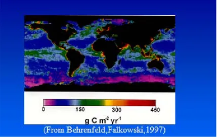
The analysis of 25 Coastal Zone Color Scanner (CZCS), derived phytoplankton pigment concentrations in Portuguese coastal waters revealed the occurrence of pigment-rich mesoscale structures which were strongly associated with the dynamics of coastal upwelling induced by favorable wind regimes along the west and the south coasts of Portugal during the summer (Sousa and Bricaud,1992).
Present studies have shown a clear pronounced nutrient dilution and contrasting Apparent Oxygen Utilization (AOU) values associated with the presence of a meddy structure in the eastern flank of Portimão Canyon off Southern Portugal. The chemical properties depict the meddy vertical extension further down the thermohaline properties, emphasizing the meddy impact on the biogeochemistry of the surrounding water masses (Brogueira et al., 2004).
3. Objective of the study
The objective of this study is to demonstrate some techniques that can be used to provide useful meteorological data, where these may be missing from conventional data sets that are provided by, for example, national meteorological authorities.
This is mainly achieved by comparison of Windguru (www.windguru.cz) data from Sagres (SW Portugal), temperature logger and wind data with the weather station data (Dr.Icely WX.stn.) at Sagres, so as to indentify upwelling events at the coastline. FERRET software is also employed to assist in substitution of the missing data. This meteorological data is related as well as assist in interpreting the biological, chemical and physical activities that occur in the coastal upwelling. The main problem is the missing data particularly in the upwelling month of August. The aim is to test the possibility of substituting windguru, computer or FERRET data for missing in situ data.
4. Research questions
This study intends to addresses following research questions:
• How much is the variation between temperature logger data derived and the observed (in situ) from Icely weather station and also between Icely weather station data and windguru data?
• How to replace missing values in the Sagres weather station data?
• Which of the two datasets (i.e Windguru and temperature logger data) is better for use to substitute the missing data to effectively assist in identifying upwelling events?
• Which methods and software used to achieve this?
5. . Materials and Methodology
Software’s used in this study include; Microsoft Office Excel 2003, SYSTAT v10, Matlab, FERRET v5.51 and Climate Predictability Tool v10.03 (CPT).
5.1.
Data Management and descriptionThe datasets comprises of: Daily temperatures, wind direction and speed, and this was obtained from Dr.Icely Weather station, at Surges records air temperature, a temperature logger attached to a signal buoy for offshore aquaculture, and this measures Sea surface temperature (SST) and the windguru dataset obtained from the website archive (www.windguru.cz), this also measure SST . These datasets, span from August to October 2009, and on daily basis. There is SST data for August 1999 from the temperature logger and this will compared with the historical Ferret mean SST for August (1946-1989). The other set of data is from the Meteorological weather station at Sagres has a lot of missing values and it is for the year 1999, and this is mainly wind
direction and speed on daily basis. This dataset is to be compared with the derived surface wind from NASA satellites by using FERRET software. There are three techniques used in this study to determine which of the dataset can best be used to replace missing values especial on the Sea surface Temperature datasets. The approaches are:
1. Plotting the daily temperature datasets in Lines on 2Axes and deturmining their skills using microsoft Excel and SYSTAT repectively.
2. Principal component regression analysis using satellite data in Climate Predictability Tool (CPT) Software;
3. Comparison with the Ferret software.
5.2.First Approach
Plotting the daily temperature datasets in Lines on 2Axes and deturmining their skills using microsoft Excel and SYSTAT repectively. Daily temperature data as well as wind direction and speed were analyzed using Excel. This was the initial data which was selected. This was done by listing the two data sets in column side by side. The first column represented date and time, the second column was for Automatic station data that is temperature logger data, the third column is the Icely weather station data and the third represents the windguru temperature data as in Table 1. From the Tables 1, 2 and 3 at the appendix C, the Icely weather station has some missing data, which needs to be replaced. SYSTAT is used to determine the skill which helps to know how the two data sets are close to each other. The software draws the histograms as well as the scatter diagrams.
5.3.SecondApproach
Replacing missing values using satellite estimates in CPT requires downloading the monthly satellite grid point data of the months one wishes to have some replacement. Note that each month needs to be handled separately, therefore you have to change the time frame to suit the name of the month you wish to download. So it may be better to download the satellite data in separate monthly files. This applicable for missing values of monthly datasets. The method used is the Principal Components Regression (PCR).The first thing is to know the boundary limits of the country or region to work on, in terms of coordinates (locations). For the Portugal coastline (Sagres) for example the locations are as follows i.e. 2°x2° apart: longitudes: 37ºN, 39ºN, 41ºN, 43ºN and latitudes: 009ºW, 011ºW, 013ºW, 015ºW. Then, the downloaded data is cut to suit the locations accordingly. The blank spaces are replaced with –999 before you run CPT as in (Table.4),at Appendix C. The first row is for stations names merged with satellite grid numbers. Second row is for Latitude, third row is for Longitude and the rest is the years and data. This is repeated for each month.
The missing values option to replace missing data is set using the nearest neighbour.For cases where there are a lot of missing values; Random numbers is the best see Fig. 4.
Fig.5. CPT Window to run the Principal Components Regression to replace the missing values for the months.
In CPT you have to put the January file as X dataset and the February File as a Y dataset. When running the inputs in CPT, they have to be in pairs as in Fig.5. Run CPT and save the input files using File –Data Output. After CPT has run, the filled file can be opened in Microsoft Excel (Table 5) at Appendix C.
5.4.Third approach
FERRET software is the main tool used in this study and can be used also to assist in filling the missing data by plotting the data and compare with the observed data for a particular day or month. In this study, derived daily surface winds at midday for August 1999 are plotted and compared as well as used where missing values are on the Sagres Meteorological data for August 1999 as well. This is an analysis tool for gridded data. FERRET is an interactive computer visualization and analysis environment designed to meet the needs of oceanographers and meteorologists analyzing large and complex gridded data sets. “Gridded data sets” in the FERRET environment may be multi-dimensional model outputs, gridded data products (e.g., climatologies), singly dimensioned arrays such as time series and profiles, and for certain classes of analysis, scattered n-tuples (optionally, grid-able using FERRET’s objective analysis
procedures). FERRET accepts data from ASCII and binary files and from two standardized, self-describing formats. FERRET’s gridded variables can be one to four dimensions usually (but not necessarily) longitude, latitude, depth, and time. The coordinates along each axis may be regularly or irregularly spaced.
FERRET offers the ability to define new variables interactively as mathematical expressions involving data set variables and abstract coordinates. Calculations may be applied over arbitrarily shaped regions. Ferret’s “external functions” framework allows external code written in FORTRAN, C, or C++ to merge seamlessly into FERRET at runtime. Using external functions, users may easily add specialized model diagnostics, advanced mathematical capabilities, and custom output formats to Ferret. A collection of general utility external functions is included with FERRET (Hankin and Denham, 1996).
FERRET provides fully documented graphics, data listings, or extractions of data to files with a single command. Without leaving the Ferret environment, graphical output may be customized to produce publication-ready graphics. Graphic representations include line plots, scatter plots, line contours, filled contours, rasters, vector arrows, polygonal regions and 3D wire frames.Graphics may be presented on a wide variety of map projections. Interfaces to integrate with 3D and animation applications, such as Vis5D and XDataSlices are also provided.Ferret has an optional point-and-click graphical user interface (GUI). The GUI is fully integrated with FERRET’s command line interface. The user may freely mix text-based commands with mouse actions (push buttons, etc.). FERRET’s journal file will log all of the actions performed during a session such that the entire session, including GUI inputs, can be replayed and edited at a later time.
Ferret was developed by the Thermal Modeling and Analysis Project (TMAP) at NOAA/PMEL in Seattle to analyze the outputs of its numerical ocean models and compare them with gridded, observational data. Model data sets are often multi-gigabyte in size with mixed 3- and 4-dimensional variables defined on staggered grids (Hankin and Denham, 1996).
Firstly, it is better to discuss how ferret works in plotting historical Meteorological parameters such as sea surface temperature (SST), air temperature (AIRT), Specific humidity (SPEH),Wind speed(WSPD), Zonal wind (UWND), Meridional wind (VWND) and Sea Level Pressure (SLP). This data is found in COADS climatologically data set using FERRET.COADS is the comprehensive ocean-atmosphere data set compiled from ship reports over the global ocean. The monthly climatology introduced here represents a simple average of all data available for each month of the year.(Hankin and Denham,1996).
6. Results and Discussion
Fig. 6 show two plots, the first one showing Icely Wx.station data versus windguru data (Fig.6A) and the second one shows Icely Wx.station data versus Temperature logger (Fig.6B) data plotted against time for the month of August. From Table 1 at the appendix C and from the graph below, it is clearly that the Icely weather station temperature data was missing at the beginning of the month up to 17th August and has highest values as compared to the other two datasets that is the Temperature logger data from the sensors in the ocean and the Windguru dataset. This is basically because it is outside the ocean on the land. It must be pointed out that land heats faster than the ocean and consequently, loses heat faster than the oceans. The mean difference between the Icely Wx.data and the other two automatic station data is about 1.7˚C,but in some cases like on 28-08-2009 the difference was 0.1˚C ,and on 25-08-2009 it was less than
0˚C i.e. at -0.1˚C. The windguru curve seems to follow the observed Icely Wx. data pattern. It must be pointed out that the Icely weather station Data measures Air temperature while the other two records SSTs.
A
B
Fig.6. plot of temperatures Icely Wx. (Sagres) versus windguru data (A) and Icely Wx. Vs Temperature logger (B)for August 2009.
Fig .7.below show the skill of the relationship of temperature datasets between the Icely weather station data at Icely Wx. Station and Windguru as well as Icely Wx. Station and temperature logger .The skill between the Sagres temperature data windguru temperature is 88% and for Sagres and temperature logger data was -14%.
Fig.7.Showing the skills between Icely Wx data at Sagres and the Windguru (88%) Left, and Temperature logger(-14%) Right, temperature datasets for August 2009.
Fig.9.Showing the skills between Windguru (-36%) and Temperature logger sea temperature datasets for August 2009.
From the plots of windguru and Temperature logger Fig.8 and 9,the skill is(-36%),implying that the skill is very low between the two datasets.
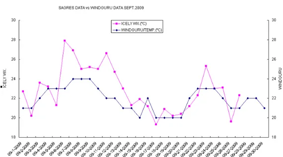
The September plots in Fig.10. has almost complete data and the difference here among the three datasets is 0.97˚C as the mean correction so to say. There some times when the temperatures coincided like on 24-09-2009 the temperature was 23˚C for both windguru data and Icely Wx.data.
B
Fig 10. Plot of temperatures of Icely Wx. Stn. versus Temperature logger (A) and Icely Wx. Stn. Vs windguru data (B) for September 2009.
The skills for the September 2009 were as follows: Icely Wx.stn. temperature and windguru 71% ,while Icely Wx.stn and Temperature logger16% ( Fig.11.) below.
Fig.11.Showing the skills between Icely Wx. Stn. and the Windguru (71%) Left and Temperature logger (16%)Right, temperature datasets for September 2009.
The windguru and the Temperature logger were in agreement throughout. The mean correction here is at 0.6˚C.
Fig12. Plot of Sea temperatures windguru data Vs Temperature logger for September 2009.
Fig14. Plot of temperatures of Icely Wx.) versus windguru data for October 2009
Similarly the plots for the October 2009, (fig.14), the trend is that as the Icely Wx. was going up and so was the windguru. The October data was only for windguru and the Icely Wx.data. The data for Temperature logger was not available and also the Icely Wx.data was missing at the beginning of the month up to October the 9th . The skill here is at 87% ( Fig.15).
Fig.15.Showing the skill( 87 Icely Wx. and the Windguru datasets for October 2009.
A comparison of the environmental data demonstrates that amongst August, September and October 2009, the windguru data was more in agreement with the other two datasets and the trend favored the Icely Wx. temperature as the Icely temperature was going up or down and so was the windguru see temperature data on the plots and also the skills were higher. Fig.6A, 7, 10B, 11, 14 and 15.
Fig.16. Wind direction and Speed (represented by the length of line) for August to October 2009.
Figure 16 shows wind direction and speed for Icely Wx.stn. from August to October 2009.The graph was constructed using Matlab software and it was predominantly of northwesterlies (NW) with maximum velocity of 36km/h occurring consecutively on August 7 and 8th .2009. The wind plot (Fig.16), indicated that the wind speed was fluctuating rising and falling but generally inclined on the rising tendency, while the wind direction was steadily northwesterly flow.
This method was also used over Sagres by (Fragoso and Icely, 2009; Loureiro et al., 2001). It is clear that the two days were upwelling periods because both the temperatures and wind regime was favorable for upwelling occurrences. The wind was
Northwesterlies and speed was high enough to effect the required Ekman transport.The temperature was 15.8˚C and 15.9˚C. respectively which is also within the specifications favourable for upwelling events.It can be noted that in the case of wind the variation is minimal as compared to the Icely weather station and the windguru. This can be confirmed by Fig.2, showing the historical three monthly averages of the Portugal currents which are wind driven. The Temperature logger from the sensor in the water showed colder temperatures explaining upwelling events during the first week and again the whole of the third week, and this was also confirmed by the Northerly westerly winds (Fig.16 and 17), with higher wind speed in the first week reaching as strong as 37km/h and so forth.
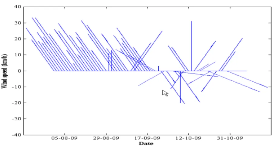
Fig.17. Wind direction and Speed (represented by the length of line) for 1999.
Fig.17. shows the plot of wind direction and speed for 1999 using Matlab software as well.The maximum velocity recorded during this period was 46km/h on 30th December 1999 and the wind direction was Northeasterlies, the temperature was 14.5˚C.The second higher velocities were recorded in the main upwelling month of August on 20th with 36km/h and the direction of North –northwesterlies (NNW) with temperature of
14.5˚C as well of and also in April the 13th at 36km/h and wind direction of Northwesterlies (NW) with 16˚C. On 1st August the velocity was at 32km/h and the direction was NW, with temperature of 14.5˚C. Similarly in this period, the main wind regime is Northwesterly component as in fig.2.This indicates that even in the case of wind, the windguru data is consistent with istu data at Sagres weather station.
The coads-climatology in Ferret contain the data variables shown in Table 6 at Appendix C.The monthly climatology introduced represent a simple average of all data available for each month of the year from 1946-1989.
In these data sets the index "I" refers to longitude, "J" to latitude, "K" to the vertical dimension, and "L" to time. In the listing the values under each qualifier present the points available along that axis. For example 1:180 indicates that locations 1 through 180 are represented in the data set.”L” refers to time in months i.e. 1:12 means January to December. Therefore if one wants to plot SST and winds for the months of January along and off the Portugal coast, in Ferret you use the following commands:
After setting and showing the data as in table 6 at Appendix C, the next step is to set the region say:
yes? SET REGION/Y=30N:50N/X=30W:4W yes? SHADE/L=1 SST
yes? GO land red
yes? VECTOR/OVERLAY/L=1 UWND,VWND
The above commands will give rise to in examples as in Fig.14,15and 16 below.Note that Y represents the longitude of the required region in this case and X is the latitude.
Fig.18. Analysis of sea surface Temperature with wind direction and speed for the month of January (1946-1989)overlaid using FERRET.
To draw the winds only, go to VECTOR/L=1 UWND,VWND and get Fig.19. below:
Fig.19. Example for the January (1946-1989) winds, plotted by FERRET.
Sagres Sagres
Fig.20. Example for the January (1946-1989)Air temperatures with contours overlaid using FERRET.
The contours for the temperature or wind direction can be overlaid on the shaded plot by using the command ‘COTOUR /OVERLAY/L=1 AIRT and this gives the plot as in Fig.20 above.
Table 8 at the Appendix C. Shows the Wind speed and direction for Meteorological station at Sagres and this was compared with the Ferret surface wind plots so as can be substituted where missing values as in the examples below: On 20th August 1999 at 12:00 hrs, the wind direction was 350˚ which was NNW and the speed in meters /second was 10m/s (Table 10 at the Appendix C). A comparison with FERRET plot of the same in time and date are agreement as can be noticed on the plots below (Fig. 21 and 22 respectively).
Fig.21. FERRET surface Winds for 20th August 1999,in vector formart.
Fig.22. Ferret surface Winds for 20th August 1999,in vector format overlaid on number of
observations(count)
N.B the arrow UWND,VWND 11.7 as indicated represent the speed of 11.7m/s as indicated on both figures and the direction of the wind is indicated by the arrow and is NNW wind ( i.e 350˚ and 10m/s as in Table 10).
Another example are on 19 and 21st August, 1999, where the data was missing and Ferret can be used to substitute those missing values as shown on Fig.23 and 24 below respectively.
Fig.23 Ferret surface Winds for 19th August 1999,in vector formart overlaid on number of
Fig.24. Ferret surface Winds for 21st August 1999,in vector formart overlaid on number of
observations(count)
Fig 25. Show the August sea temperature from the temperature logger at Sagres.The temperature was between 13˚ to 17˚C,which was favarable for upwelling.
Deductions from Fig.21,22, 23, 24 and 25 is that wind regime together with that at Sagres favor upwelling as evidenced from the wind to the north of the Sagres coast is divergent implying that water was moving apart which is one of the mechanism that causes upwelling.
A comparison of the environmental data demonstrates that between May and September the strong fluctuations in sea surface temperature (SST) are related to wind events with lower temperatures occurring after periods of dominant north-westerly winds. Similar observations have been made for this region in previous studies (e.g. Fiúza, 1983; Loureiro et al., 2005). The comparisons done by other studies, evidence that the Sagres winds are spatially more confined and exhibit a stronger spatial heterogeneity than the winds at Sines. The zone of maximum correlation extends concentrically around Cape St. Vincent (Sãnchez et al., 2007).
7. Conclusions
The skill tests between the Icely Wx.stn air temperature data and Windguru as well as temperature logger indicate that the Windguru data is a good substitute of missing values on the Icely Wx.stn (in situ data) as well as the Meteorological weather data because it showed very high skill as compared to the temperature logger data. Besides, has the same trend with Icely Wx.stn.temperature, as the Icely temperature data was going up or down, and so was the Windguru data on the plots. Comparison between windguru and temperature logger, proved that the two dataset are not related as can be deduced from the very low negative skills.
The Ferret analysis has proved also to be a good tool for making substitution to the missing Meteorological data as evidenced by the daily comparisons with the August1999 Ferret derived surface winds and Meteorological wind dataset for Sagres. There is classical view that in this region favourable winds force near-surface offshore transport and coherent flow along the coast, does not apply throughout the upwelling season (Relvas and Barton,2005). Other methods may still be utilized where the Ferret tool fails to meet the expectation, this in the case of non-availability of data for the Ferret software. These considerations can alleviate the difficulties in explaining the biological and chemical process that take place along the Sagres coastline such as upwelling events.
8.References
Bischof, B., Mariano, A. J., Ryan. E.H. (2003). "The Portugal Current System." Ocean Surface Currents (http://oceancurrents.rsmas.miami.edu/atlantic/portugal.html)
Barton, E. (2001). Canary and Portugal currents. University of Wales, Bangor, UK. Copyright Academic Press doi:10.1006/rwos.2001.0360.
Bettencourt, A. M., Bricker, S. B., Ferreira, J.G., Franco. A., Marques, J.C., Melo, J.J., Nobre, A., Ramos, L., Reis,C.S., Salas, F., Silva, M.C., Simas, T., Wolff W.J.(2004).Typology and Reference conditions for Portuguese Transitional and Coastal Waters, Development of Guidelines for the Application of the European Union Water Framework Directive, INAG and IMAR, Lisbon, Portugal. 98p.
Brogueira M. J., Cabeçadas G., Gonçalves C. (2004) Chemical resolution of a meddy emerging off southern Portugal, Continental Shelf Research. 24: 1651-1657. ISSN 0278-4343
Conway, E. D. (1997). An introduction to satellite image interpretation, Johns Hopkins Univ. Pr. Maryland Space Grant Consortium, The Johns Hopkins University Press, Baltimore, 242 p. ISBN 0 8018 5576 4.
Detlefsen, H. and P. Speth.(1980). Investigations on coastal upwelling off Northwest Africa and Portugal with empirical orthogonal functions, Journal Ocean Dynamics. 33: 210-221.
Fiúza,A.F.G.,M.E. Macedo and M.R. Guerreiro,(1982). Climatological space and time Variation of the Portuguese coastal upwelling. Oceanol.Acta, 5(1): 31-40 Fiúza, A.F.G., 1983. Upwelling patterns off Portugal. In: Suess, E., Thiede, J. (Eds.),
Coastal Upwelling: its Sedimentary Record. Part A. Responses of the
Sedimentary Regime to Present Coast Upwelling. Plenum, New York, 85–98 p. Fragoso, B. and J. D. Icely (2009). Upwelling Events and Recruitment Patterns of the
Major Fouling Species on Coastal Aquaculture (Sagres, Portugal). Journal of Coastal Research,SI 56 (Proceedings of the 10th International Coastal Symposium),419-423.Lisbon,Portugal,ISSN 0749-0258.
Hankin, S and Denham, M (1996). FERRET User's guide, NOAA/PMEL/TMAP (1996) Version 4.4.
Harimoto, T., Ishizaka, J., Tsuda, R.(1999).Latitudinal and vertical distributions of phytoplankton absorption spectra in the central North Pacific during spring 1994,. Journal of Oceanography, Volume 55, Number 6, December 1999 , 667-679(13) pp.
Loureiro, S., Newton, A., Icely, J.D.(2001). Microplankton composition, production and upwelling dynamics in Sagres (SW Portugal) during the summer of 2001.Scientia Marina, 69. 323-341.
Loureiro, S., Newton, A, Icely, J.D. (2005). Microplankton composition, production and upwelling dynamics in Sagres (SW Portugal) during summer of 2001. Scientia Marina, 69. 323-341.
Loureiro, S., Icely, J.D., Newton, A. (2008). Enrichment experiments and primary production at Sagres (SW Portugal), Journal of Experimental Biology and Ecology, 359, 119-125.
Martins, C. S.,Hamann,M.,Fiúza,A.F.G.(2002). Surface circulation in the eastern North Atlantic, from drifters and altimetry, Journal of Geophysical Research, 107, 3217, doi: 10.1029/2000JC000345.
Peliz, A. J.,Fiúza, A. F. G.Za. (2001). Temporal and spatial variability of CZCS-derived phytoplankton pigment concentrations off the western Iberian Peninsula. International Journal of Remote sensing 7,1363-1403.
Perez, Fiúza F., C. G. Castro, X. A. Alvaréz-Salgado, A. F. Rios (2001). Coupling between the Iberian basin-scale circulation and the Portugal boundary current system: a chemical study, Deep-Sea Research I, 48, 1519-1533.
Relvas, P., Barton, E.D. (2002). Mesoscale patterns in the Cape São Vicente (Iberian Peninsula). Journal of Geophysics Research. 107, 3164, doi:
Relvas,P., Barton, E.D., Dubert,J., Oliveira,P.B., Peliz, Da Silva,J.C.B.,Santos, A.M.P. (2007). Physical oceanography of the western Iberia ecosystem: Latest views and challenges,Progress in Oceanography Vol.74: 149–173.
Sãnchez, R. F., Relvas, P. ,Pires,H.O. (2007). Comparisons of ocean scatterometer and anemometer winds off the southwestern Iberian Peninsula, Cont Shelf Res 27:155–175.
Santos, A. M. P, de Fátima Borges, M.; Groom,S. (2001). Sardine and horse mackerel recruitment and upwelling off Portugal. Fisheries Research, Vol. 58: 589. Instituto de Investigação das Pescas.
Solignac, S.,de Vernal, A.,Giraudeau,J. (2008). Comparison of coccolith and dinocyst assemblages in the northern North Atlantic: How well do they relate with surface hydrography?, Marine Micropaleontology, 68, 115-135.
Sousa, F. M. and A. Bricaud, (1992). Satellite-derived phytoplankton pigment structures in the Portuguese upwelling area, Journal of Geophysical Research 97, 11343-11356.
Villa, H., Quintela, J., Coelho, M.L., Icely, J.D., Andrade,J.P. (1997). Phytoplankton biomass and zooplankton abundance on the south coast of Portugal (Sagres), with special reference to spawning of Loligo vulgaris. Scientia Marina. 61: 123-129.
Wollast R. (1998). Evaluation and comparison of the global carbon cycle in the coastal zone and in the open ocean, In: The Sea: The Global Coastal Ocean: Processes and Methods. Brink, K.H. and A. R. Robinson, eds. Vol. 10. John Wiley & Sons, Inc. N.Y. 213-252 pp.
Wooster, W.S., Bakun, A., McLain, D.R., 1976. The seasonal upwelling cycle along the
eastern boundary of the North Atlantic. J. Mar. Res. 34 (2), 131–141.
Appendix A. Review of Oceanographic and Meteorological
Processes responsible for coastal upwelling.
1. Review
Global climate coupled ocean-atmospheric phenomena such as El Niño Southern Oscillation(Picaut et al.,1996),commonly known as El Niño / La Niña and the North Atlantic oscillation (NAO) plays an important role in the fluctuations of atmospheric processes. Sea Surface Temperature (SST) fluctuations of the tropical Eastern Pacific
Ocean occur in the case of El Niño Southern Oscillation (ENSO) and atmospheric pressure at sea-level difference between the Icelandic Low and the Azores High takes place during the North Atlantic Oscillation (NAO).
Upwelling of ocean water is affected by wind. As wind moves across the surface layer the water is dragged along due to frictional force and this top layer of water is pulled along in the same direction as the wind. Wind-driven upwelling systems are part of the coastal upwelling occurring along the Portuguese coastline, the western coasts of the Iberian Peninsula and Africa down to 15°N (Relvas and Barton,2002) Fig.1at Appendix B, shows the areas major upwelling in the world.
On an annual-mean basis, very warm surface water of about 29.8C occupies most of the area between 78N and 108S, 1308E and 1708W (Picaut et al.,1996), Fig.2. at Appendix B, Showing cold and warm water currents. Oceanography enables Oceanographers to forecast sea state in the same way that Meteorologists forecast the atmosphere today. Ocean state and wave height help the sailors to choose the best route, thus saving the valuable time.The distinct Pattern Of ocean-atmosphere relationship is associated with interdecadal variability in the North Atlantic region. The middle- and high-latitude sea surface temperatures (SST) display a long-term fluctuation with negative anomalies before 1920, and during the 1970s and 1980s. Positive SST conditions prevailed from about 1930 to 1960
.
(Kushnir, 1994).
In the North Atlantic mid ocean area, an anomalous cyclonic circulation prevailed during years with warm SST, and an anticyclonic anomaly dominated during years with cold SST. These circulation anomalies are strongest during the winter months (Kushnir,1994).Satellite infrared sensors only observe the temperature of the skin of the ocean rather than the bulk sea surface temperature (SST) traditionally measured from ships and buoys. In order to examine the differences and similarities between skin and bulk
temperatures, radiometric measurements of skin temperature were made in the North Atlantic Ocean from a research vessel along with coincident measurements of subsurface bulk temperatures, radiative fluxes, and meteorological variables. Recommendations were made to calibrate satellite derived SST's during night with buoy measurements and the additional aid of meteorological variables to properly handle temperature difference variations (Schluessel et al.,1990 ).
Chlorophyll patchiness caused by mesoscale upwelling at fronts were detected in the open North Atlantic during summer (Strass,1992). The mesoscale patches with highest chlorophyll concentrations occur at those sites where the hydrographic conditions are favorable for dynamic upwelling or where the distributions of the hydrographic variables indicate local upwelling events (Strass, 1992).
2.Global Climate-Coupled Ocean-atmospheric
The general circulation of the atmosphere imbeddes the hydrological cycle.Water balance at the surface and subsuface is strongly coupled with the patterns and behavior of the climatic system and the capability to simulate and predic the general circulation of the atmospheric fluid is thus of great importance to hydrology. Climatic general circulation models (GCMs) have been devised to produce the basic patterns and processes in the atmospheric system (Entekhabi, 1990).
2.1. El Niño Southern Oscillation (ENSO)
The El Niño Southern Oscillation (ENSO) represents the largest signal in inter-annual climate variation, affecting global atmospheric and oceanic circulation patterns. The phenomenon undergoes cycles between warm ENSO conditions (which are extreme during El Niño episodes) and cold ENSO conditions (extreme during La Nina episodes) (Viboud et al., 2004). Recent developments in the El Niño-Southern Oscillation
(ENSO) phenomenon have raised concerns about climate change. El Niño and La Niña are major temperature fluctuations in the tropical Pacific Ocean (see Fig.3), at Appendix B. They are Pacific signatures of the global ENSO phenomenon (El Niño-Southern Oscillation). Their effect on climate in the southern hemisphere is profound. Their role in global warming or cooling is an area of active research, with no clear consensus yet. Fig 4 at Appendix B.ENSO-Neutral conditions (a) compared to the warmer waters of a typical El Nino.
(b) Shown as sea surface temperature anomalies in the equatorial pacific ocean. The atmospheric signature, the Southern Oscillation (SO) reflects the monthly or seasonal fluctuations in the air pressure difference between Tahiti and Darwin. Fig.5 at Appendix B.
2.1.1. El Niño Southern Oscillation (ENSO) Index
Fluctuations in tropical Pacific sea surface temperature (SST) are related to the occurrence of El Niño, during which the equatorial surface waters warm considerably from the International Date Line to the western coast of South America (Stenseth, et al., 2003). However, it is important to remember that the pattern of relationship between SOI and rainfall (and temperature) can vary depending on the particular season and region. Additionally, the change in SOI over a specified period can be as important in understanding relationships between SOI and rainfall as is the absolute value in SOI. See fig.5. at Appendix B. Predictions of ENSO are done at International Prediction centers such as the IRI ( International Research Institute for climate and society).Fig.6. at Appendix B and Table 9 at appendix C show ENSO probabilistic forecast for NINO3.4 Region.
2.1.2.El Nińo
El Niño is an unusual warming of the ocean surface waters in the Eastern Pacific Ocean(Trenberth, 1997). This brings a lot of rains in other areas of the world and at the same time bring less rainfall or drought in other parts as well,in other words it can be reffered to as a circlic event. Fig.7 at Appendix B illustrates the above.
2.1.3. La Niña
La Niña is the name for the cold phase of ENSO, during which the cold pool in the
eastern Pacific intensifies and the trade winds strengthen. The name La Niña originates from Spanish, meaning "the little girl", analogous to El Niño meaning "the little boy (Trenberth, 1997). La Niña is just the flipside of El Niño (Fig.7); La Niña tends to follow the El Niño. In 1997-1998, the biggest El Niño on record killed thousands of people (Ellison, 2009).
3. Ocean winds and circulation
Wind plays an important role in the air-sea interaction between sea surface temperature and upwelling. Wind regulates the temperature of seawater by transporting the heat across the water surface.The Sea Surface Temperature (SST) decreases at the beginning of the upwelling season, reaches its peak in May-June, corresponding with the winds, but starts rising in July due to increased solar heating at the surface, combined with the decreased alongshore winds in Central California (Diehl et al.,2007).
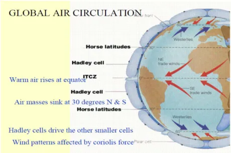
Trade winds are part of the atmospheric general circulations which drives the ocean currents (Fig.8 and Fig.9),at Appendix B, show the general circulation and wind effect on surface water currents respectively).Wind regulates the temperature of seawaters by
transporting heat across the water surface in form of land and sea breezes on a localized scale and through oceanic currents on large scale extent. Very high resolution radiometer (AVHRR) satellite images of sea surface temperature and time series of sea level height, wind velocities, and near shore sea surface temperature was studied and
recorded at coastal sites within 200km of Cape São Vicente (Relvas and Barton,2002).
3.1.Ocean Surface Circulation
The westerlies are associated with heavy rainfall and thunderstorms in tropical Africa. The boundary between the northwesterly winds and the northeasterlies (northeast trade winds)is known as the Congo air boundary and it is associated with rainfall and thunderstorms. The convergence between the north east trade winds and the southeast trade winds is commonly known as the Inter Tropical Convergence Zone (ITCZ). The ITCZ is the main rain mechanism in most parts in the tropics. The trade winds (also called trades) are the prevailing pattern of easterly surface winds found in the tropics near the Earth's equator. The trade winds blow predominantly from the northeast in the Northern Hemisphere and from the southeast in the Southern Hemisphere. The trade winds act as the steering flow for tropical storms that form over the Atlantic, Pacific, and Indian Oceans that make landfall in North America, Southeast Asia, and India, respectively. Trade winds also steer African dust westward across the Atlantic ocean into the Caribbean sea, as well as portions of southeast North America.Fig.10, at Appendix B showing the trade winds as part of the Earth's atmospheric circulation. During an El Niño event, however, the trade winds weaken and the coastal upwelling diminishes, (Conway, 1997).
The NAO is a large scale seesaw in atmospheric mass between the subtropical high and the polar low. The corresponding index varies from year to year, but also exhibits a
tendency to remain in one phase for intervals lasting several years.(Hurrell et al., 2003).The surface ocean currents circulations are powered by the prevailing winds. The forces that drive and direct the movement of the oceanic currents are: Wind, Coriolis force, Gravity and Friction .The circulations in the Northern Hemisphere are clockwise while in the southern Hemisphere is anticlockwise see Fig.11, at Appendix B. It is suspected that global warming might have a significant effect on the currents; see Fig.11 for details.
4. Northern Atlantic Winds
Wind circulation over the northern Atlantic ocean is associated with northern Atlantic upwelling system of western coast of the Iberian Peninsula (Peliz et al., 2002) and the coastal upwelling region near Cape São Vicente (Relvas and Barton,2002).
In the Northern Atlantic, as the Gulf Stream flows north, it encounters the Labrador flowing south along the banks of Cape Hatteras. As these two currents meet, they begin to meander (they wind back and forth like a snake). Eventually, these meanders "pinch off" from the main flow and become independently rotating structures, known as rings.(see Fig.12 at Appendix B).These are the warm core rings and the cold core rings, previously known as eddies.
4.1. Northern Atlantic Oscillation (NAO)
This north Atlantic circulation is known as “The North Atlantic oscillation (NAO)”.This is a climatic phenomenon in the North Atlantic Ocean of fluctuations in the difference ofatmospheric pressure at sea-level between the Icelandic Low and the Azores high. Through east-west oscillation motions of the Icelandic Low and the Azores high, it controls the strength and direction of westerly winds and storm tracks across the North Atlantic (Stenseth et al.,2003). It is highly correlated with the Arctic oscillation, as it is
a part of it (see Fig.13 at Appendix B). The NAO was discovered in the 1920s by Sir Gilbert Walker. Unlike the El Niño phenomenon in the Pacific Ocean, the NAO is a largely atmospheric mode. It is one of the most important manifestations of climate fluctuations in the North Atlantic and surrounding humid climates. The North Atlantic Oscillation is closely related to the Arctic oscillation but should not be confused with the Oscillation Westerly winds blowing across the Atlantic, bring moist air into Europe. In years when westerlies are strong, summers are cool, winters are mild and rain is frequent. If westerlies are suppressed, the temperature is more extreme in summer and winter leading to heatwaves, deep freezes and reduced rainfall.The North Atlantic Current (North Atlantic Drift and the North Atlantic Sea Movement) is a powerful warm ocean current that continues the Gulf Stream northeast. West of Ireland it splits in two. One branch (the Canary Current) goes south while the other continues north along the coast of northwestern Europe where it has a considerable warming influence on the climate. Other branches include the Irminger Current and the Norwegian Current. Driven by the global thermohaline circulation (THC), the North Atlantic Current is also often considered part of the wind-driven Gulf Stream which goes further east and north from the North American coast, across the Atlantic and into the Arctic Ocean.
The variations in seasonal rainfall in Southern Europe during the present century, has relationships with the North Atlantic Oscillation (NAO) and the El Niño-Southern Oscillation (Stenseth et al., 2003).
4.2 Northern Atlantic Oscillation Index (NAOI)
It is known from observations that the North Atlantic Oscillation(NAO) is the dominant, large-scale, extra-tropical teleconnection pattern in the Atlantic sector (Bjerknes,1964; Hurrell and Van Loon, 1997). Its phase is indicated by the NAO index (NAOI), which