Hydrogen Permeation in Parabolic Trough Receivers

(1)

Hydrogen Permeation in

Parabolic Trough Receivers

Helena Mafalda de Sousa Reis Orvalho

M A S T E R T H E S I S

submitted in Faculdade de Ciencias e Tecnologia da Universidade Nova de Lisboa, in partial fulﬁllment of the requirements for the degree of

Master in

Materials Engineering

Monte da Caparica,

July 2009

Supervised by:

(2)

Acknowledgements

First I would like to thank Professor Isabel Ferreira for taking time out from her busy schedule, agree to be my Supervisor and opening the door to such fantastic opportunity.

I’m also indebted to my external supervisor Dr Marc Moellenhoﬀ for making himself always available, giving great advice and encouragment even though he was often buried with work.

I also want to express my gratitude to Tim Gnaedig, Zdenek Hacker, Dr Jan Schulte-Fischedick and Matthias Mueller whose expertise, understanding, and patience helped me to go through all the diﬃculties faced.I wish also to thank Christina Albers for taking the trouble of reading thoroughly the thesis and making suggestions.

I’m also grateful to all the workshop staﬀ especially Matthias Mueller, Rino, Adolf, Karl-Heinz, Gerald and Sebastian for all the assistance provided in the building process.

I must also thank my colleagues and friends : Jens, Sulivan, Michael, Klaus, Soﬁa, Kamel, Se-bastian, Marc, Zdenec, Stefan, Alex, Celia and Matthias not only for a great work environment but also for making me feel i was at home.

I won’t ever be able to convey my appreciation fully to Matthias and Marion Mueller for taken me under their wing during the time i’ve been in Mitterteich: I owe them my eternal gratitude for everything they did.

Finally a very special thanks to my family for their unconditional love and support not only during the time of this thesis but throughout my life, without which I wouldn’t be able to have gone this far.

(3)

Abstract

The continued economic and population development puts additional pressure on the already scarce energetic sources. Thus there is a growing urge to adopt a sustainable plan able to meet the present and future energetic demands.

Since the last two decades, solar trough technology has been demonstrating to be a reliable alternative to fossil fuels. Currently, the trough industry seeks, by optimizing energy conversion, to drive the cost of electricity down and therefore to place itself as main player in the next energetic age.

One of the issues that lately have gained considerable relevance came from the observation of signiﬁcant heat losses in a large number of receiver modules. These heat losses were attributed to slow permeation of traces of hydrogen gas through the steel tube wall into the vacuum annu-lus. The presence of hydrogen gas in the absorber tube results from the decomposition of heat transfer ﬂuid due to the long-term exposure to 400°C.

The permeated hydrogen acts as heat conduction mean leading to a decrease in the receivers per-formance and thus its lifetime. In order to prevent hydrogen accumulation, it has been common practice to incorporate hydrogen getters in the vacuum annulus of the receivers. Nevertheless these materials are not only expensive but their gas absorbing capacity can be insuﬃcient to assure the required level of vacuum for the receivers to function.

In this work the building of a permeation measurement device, vulnerabilities detected in the construction process and its overcome are described. Furthermore an experimental procedure was optimized and the obtained permeability results, of diﬀerent samples were evaluated. The data was compared to measurements performed by an external entity. The reliability of the com-parative data was also addressed.

In the end conclusions on the permeability results for the diﬀerent samples characteristics, fea-sibility of the measurement device are drawn and recommendations on future line of work were made.

(4)

Notation

List of frequently used symbols

a activity c concentration

c1 concentration at the feed side c2 concentration at the permeate

side

di inner diameter

do outer diameter

k Boltzmann constant l thickness

m mass in g

n number of particles in mol r pressure exponent

s pumping speed t time

u drift velocity x coordinate y ordinate

A area

Ais inner superﬁcial area

Ar molar mass in g/mol B mobility

C ﬁt parameter D diﬀusivity

D0 pre-exponential factor ofD F force

G capacity if the getter

H activation energy

HD,HS,Hφ activation energy ofD,S and

φ

K compression ratio

J ﬂux

L lenght

M metal

P pressure

P0 pre-exponential factor ofP Q gas ﬂow (general term)

Q0 outgassing ﬂow

QT throughput

Qφ permeation gas ﬂow

R universal gas constant

S solubility

S0 pre-exponential factor ofS

T temperature

U potential

V volume

W ﬁt parameter

Z ﬁt parameter

φ permeability

φ0 pre-exponential factor ofφ µ chemical potential

µ0 _{standard chemical potential} at standard conditions, T = 298,15 K;P = 101325 Pa

(5)

Notation iv

Subscripts

Bo grain boundary

G grain

Gter getter

List of Abbreviations and Acronyms

bcc body centered cubic fcc face centered cubic hcp hexagonal closed packed ASS austenitic stainless steel CMR capacitance diaphragm gauge DPO diphenyl oxide

HCE heat conductive element HS heating system

HTF heat transfer ﬂuid HV high vacuum

IPP Institute fuer Plasma Physik LD literature data

PID proportional integral derivative controller PKR full range gauge

PMD permeation measurement device PS pumping stage

PTPP parabolic trough power plant QMS quadrupol mass spectrometer RVP rotary vane pump

TP turbo molecular pump UHV ultra high vacuum VA vacum annulus

(6)

Notation v

Vacuum Symbols

KF connection

CF connection

ﬂexible connection

feedtrough

pressure gauge

corner valve

needle valve

manual valve

rotary vane pump

(7)

List of Figures

1.1 Concentrated Solar Thermal Technologies . . . 2

1.2 Concentration type and working temperature of solar thermal technologies . . . . 3

1.3 Schotts PTR 70 Receiver . . . 4

1.4 Components of the Heat Transfer Fluid . . . 5

1.5 Cleavage reactions of biphenyl . . . 6

1.6 Cleavage reactions of DPO . . . 6

2.1 Deﬁnition of the ﬂux . . . 8

2.2 FCC structure . . . 9

2.3 One dimensional description of Fick’s laws . . . 12

2.4 Mechanisms of diﬀusion . . . 13

2.5 Schematic of the mechanism of permeation for two atomic gases . . . 14

3.1 Measuring chambers in the ﬁnal permeation device . . . 19

3.2 Final Permeation Measurement Device Scheme . . . 20

3.3 Turbo pump section . . . 21

3.4 Rotary Vane Pump schematic representation . . . 22

3.5 Isolation between the heating system and heating wire . . . 23

3.6 Initial and ﬁnal heating system . . . 24

3.7 PID loop tuning temperature curves . . . 25

3.8 Samples surface temperature curve for the initial heating system . . . 26

3.9 Samples surface temperature curve for the late heating system . . . 26

3.10 Functioning Principle of QMS 200 . . . 27

3.11 QMS measurement proﬁle . . . 28

3.12 Diaphragm capacitive gauges working principle . . . 29

3.13 Pirani Circuit . . . 29

3.14 Penning Gauge . . . 30

3.15 Cause eﬀect diagram of the main problems faced . . . 31

3.16 Behaviour of the heating parts in consecutive trials . . . 33

3.17 Inﬂuence of the TP breakdown in the measurement results . . . 34

3.18 Contamination of the cathode of the full range gauge . . . 35

3.19 Assembled probe . . . 36

3.20 Detailed view of a measuring chamber, full range gauge positioning, intermediary pipping and ﬂow direction . . . 37

3.21 Measurement proﬁle and stage identiﬁcation . . . 37

3.22 Temperature Proﬁle of the sample in chamber 1 . . . 40

3.23 Temperature Proﬁle of the sample in chamber 2 . . . 40

4.1 IPP Permeation Measurement Device . . . 42

4.2 Producer A flux versus time curves . . . 44 4.3 Producer D flux versus time curves, average curve fitting and respective parameters 44

(10)

LIST OF FIGURES ix

(11)

List of Tables

1.1 Status of Concentrated Solar Power Overview in 2007 . . . 3

3.1 Turbomolecular pump characteristics . . . 22

3.2 Rotary Vane Pump models, pumping speed for nitrogen and ultimate pressure . . 23

3.3 Eﬀects on increasing Parameters . . . 24

3.4 Temperatures along the Sample and average for each chamber . . . 41

4.1 Flux and permeability for the experimental results . . . 45

4.2 Relative Errors . . . 45

6.1 Diﬀerences between initial and current permeation measurement devices . . . 50

(12)

Chapter 1

Introduction

An overwhelming consensus of scientiﬁc opinion agrees human activities, such as burning fossil fuels, are responsible for the relentless build-up of greenhouse gases in the earth’s atmosphere and consequent global climate change. This process is already disrupting ecosystems and through the increasing risk of hunger, diseases, ﬂooding and water shortages is estimated to be causing around 150,000 additional deaths per year and threatening millions of people [1].

On the other hand, fossil fuels - oil gas and coal - are becoming scarcer and more expensive to produce. This adding to the over-reliance on energy imports from a few, often politically un-stable countries contribute to the increasing social and economical instability.

If this present perspectives seem already dark, the future is not also much brighter. The devel-opment of global energy demand is driven by two key factors:

• Population development: according to the United Nations population development projec-tions, the world’s population is expected to grow from 6,3 to almost 8,9 billion [1] by 0,78% over the period 2003 to 2050.

• Industrial development and economic growth

This scenario reveals the unfeasibility of our actual energetic plan and drives us to the evident conclusion that, sooner or later, it will have to change.

Renewable energies provide a real and mature solution to our future that combined with the smart use of energy can deliver half of the worlds needs by 2050. [1]

1.1 Concentrated Solar Thermal Technology

Over 99.9% of the available ﬂow of renewable energy on Earth is constituted by resources such as wind and wave power, hydroelectricity, biomass and solar radiation.

Solar radiation consists of direct and diﬀuse irradiation. If the skies are overcast, only diﬀuse radiance is available.

Direct solar radiation reaches the earth surface with a density (kW/m2_{) adequate for heating} systems but not for an eﬃcient thermodynamic cycle to produce electricity. The density has thus to be increased, through the use of mirrors or lenses that concentrate the incoming solar radiation in a point or along a line. The most common types of concentrating solar thermal systems are shown in ﬁgures 1.1 and 1.2. We have:

(13)

Chapter 1. Introduction 2

Figure 1.1: Concentrated Solar Thermal Technologies; top: Power Tower power plant PS10 in Sanlucar, Spain [2] (left) and Dish Stirling modules in Solar Two, California, USA [3] (right); bottom: Fresnel [4] (left) and Parabolic Troughs [4] (right) in Plataforma Solar de Almeria, Spain

1. Power tower systems that consist of ﬁelds where thousands of sun-tracking mirrors (he-liostats) direct insolation to a receiver. The receiver is placed on top of a tall tower where a molten salt heat-transfer ﬂuid is heated and driven to the ground based steam generator. The steam drives then turbines that activate the generator and electricity is produced.

2. Dish Stirling systems that generate power by using parabolically arranged mirrors to reﬂect sunlight onto a small focal receiver, the stirling engine, thereby heating a gas chamber connected to a piston and drive shaft. The drive shaft powers a generator and produces electricity.

3. Fresnel technology uses horizontal ﬂat mirror facets that track the sun. The energy is also transferred to a heat exchanger using a heat transfer medium

4. Parabolic troughs where rows of trough-shaped mirrors direct insolation to a receiver tube placed along its focal axis. The focused radiation heats the heat-transfer ﬂuid (HTF) which goes through a heat exchanger that generates steam and powers the conventional turbines.

Table 1.1 gives an overview of the maturity status of each concentrated solar power system.

(14)

Table 1.1:Status of Concentrated Solar Power Overview in 2007 [5]

Technology Status Projects ahead Location

Parabolic Trough Commercial 50-150 MW

Spain, India, Mexico, Egypt, Morocco, Crete, Jordan, USA, South Africa

Linear Fresnel Prototype, 1-5 MW pilot plant California demonstration

Solar Power Tower Prototype, PS10 (10 MW steam cycle) Spain demonstration

Parabolic Dish

Prototype, EURO-DISH, 10 kW series, California, USA demonstration Solar One and Two, 500

and 850 MW Power Plant

Solar Receiver Heliostats Absorber Tube Pipe with thermal fluid Curved mirror

Receiver / Engine

Absorber tube and reconcentrator Curved mirror Solar Receiver Heliostats Solar Receiver Heliostats Absorber Tube Pipewith

thermalfluid

Curved mirror

Receiver / Engine

Reflector Receiver / Engine

Absorbertube and reconcentrator

Curved mirror

Linear Concentration

T ~ 300-500° C

Point Concentration

T ~ 1000° C

a) Parabolic Trough b) Linear Fresnel

c) Dish Stirling d) Power Tower

Figure 1.2:Concentration type and working temperature of solar thermal technologies [6]; Linear concentration technologies operate in temperatures ranging 300-500ºC while point concentration technologies in temperatures around 1000ºC

There is also a possibility of combining solar thermal power plants with fossil energy sources. Since solar ﬁelds feed their heat energy into a conventional steam turbine, they can be easily integrated in latest generation and relatively clean, natural gas ﬁred combined cycle power plants.

1.2 Parabolic Trough Technology

Parabolic trough technology has the highest eﬃciency at lowest energy production costs and material requirements of all solar thermal power plant technologies.

(15)

is also a proven technology that has already achieved market maturity and shown its reliability: the first PTPP was built in Mojave´s Desert in 1984. By 1991, nine solar fields with 2,5 million square meters of concentrating reflector surface were erected on more than 7 km2_{. So far they} have been running with a total output of 354 MW and fed more than 12 billion kW hours into the California grid, earning nearly 1,6 billion US dollars. Its technical availability has always been over 98 percent and the 25 years planned lifetime of the parabolic trough field is expected to be exceeded by far [7].

1.3 Brief Presentation of the Company and Product

Schott is a 125 year old multinational, technology-based group that develops and manufactures specialty materials, components and systems for diverse markets: household appliances, pharma-ceutical industries, electronics, optics, automotive and solar energy.

Figure 1.3: Schotts PTR 70 Receiver [8]; it consists of an ab-sorber tube enclosed in vacuum by a glass tube with metallic bellows and seal

The business unit Schott Solar AG is one of the leading solar industry companies worldwide. It oﬀers a wide range of future-oriented products and solutions for almost all photovoltaic and solar thermal applications.

In the segment of concentrated solar power, SCHOTT Solar CSP GmbH oﬀers high-output receivers (ﬁgure 1.3) that are a key component in solar thermal parabolic trough power plants.

1.3.1 Schott Solar Trough Receivers

The receivers, also known as heat conductive elements (HCE), consist of an absorber tube en-closed in vacuum by a glass tube.

The absorber tube is 4 meter long austenitic stainless steel (ASS) tube with a multilayer solar-selective absorber surface.

The cermet absorber coating is produced in a reactive sputtering and its optical properties allow to achieve high solar absorbance and low emittance at the HCE working temperatures, maxi-mizing solar gains and minimaxi-mizing heat losses.

The glass tube is coated with anti-reflective films for high solar transmittance on both sur-faces to minimize the reflective losses and maximize the solar transmittance.

The vacuum pressure in the vacuum annulus (VA) is kept below 0,1 Pa to suppress heat con-duction losses. To maintain such vacuum levels, getters designed to absorb gas molecules, are installed in the vacuum space. The receivers also include an evaporable barium getter used to monitor the vacuum in the receiver. The barium getter presents a silver appearance that turns white if the vacuum level is compromised.

(16)

1.4 Hydrogen Problematic

Observations in several solar ﬁelds [9] have revealed signiﬁcant heat losses in a large number of receiver modules. These heat losses have been attributed to the slow permeation of gas traces through the steel tube wall into the VA, compromising its thermal insulation capacity and thereby shortening the receivers lifetime. In order to absorb these traces of hydrogen gas formed over time it has been common practice to incorporate hydrogen getters in the VA. However these materials are expensive and the long-term exposure of the organic thermal oil to 400°C can lead to hydrogen pressures that exceed the getters gas-absorbing capacity.

1.4.1 Thermal Decomposition of the Heat Transfer Fluid

The HTF that ﬂows inside of the HCE, is known under the trademark of Therminol VP-1 or Dowtherm A. Its composition is 73,5% diphenyl oxide (DPO) and 26,5% biphenyl in the eutectic formulation [10]. In spite of having a boiling point of 257°C, the HTF has been successfully

O

diphenyl oxide biphenyl

Figure 1.4: Components of the Heat Transfer Fluid [10]; diphenyl oxide and biphenyl

used above this temperature in PTPP for many years without a signiﬁcant decrease in the performance. This might be due to its low thermal degradation rates as it was study in reference [11]. In this work, Dowtherm A was heated at 425°C for 120 h which resulted in the formation of a mixture composed by: a) gaseous products consisting of hydrogen gas, 44% of the total gas volume, and small hydrocarbons, and b) a fraction containing the aromatic compounds.

Thermal Decomposition of Biphenyl and DPO

The direct thermal cleavage of biphenyl and diphenyl oxide (ﬁgure 1.6) forms phenyl radicals, and phenoxy [12, 13]. The resultant highly reactive hydrogen atoms may either recombine or attack the biphenyl and DPO. These steps altogether can then initiate a chain reaction leading to the production of benzene, polyphenyl compounds (e.g. terphenyl), and also more hydrogen atoms that ultimately recombine to form hydrogen gas [14] as it is shown in ﬁgures 1.5 and 1.6.

Hydrogen Pressures in Parabolic Trough Receivers

(17)

+

H + +

H

terphenyl

2 H H₂

Figure 1.5:Cleavage reactions of biphenyl [10]; either by highly reactive hydrogen atoms (first re-action), thermal cleavage (second reaction) and consequent formation of poliphenyls and molecular hydrogen

O

O O +

H ₊

O

(18)

1.5 Aim of the Present Work

The aims of the present work were:

• to put up a permeation measurement equipment,

• the assessment of its reliability through the evaluation of the measurement results,

The ability of measuring the permeability constitutes the ﬁrst step towards the development of permeation resistant barriers. An eﬀective permeation barrier will then allow the reduction of heat losses and necessary getter amount required to keep the receivers running for 25 years.

This thesis is the follow up of works which came up with a prototype of a permeation mea-surement device (PMD).

The prototype was rebuilt in this work and subjected to a longer period of testing that helped to identify and resolve its main limitations. Chapter 3 presents the methods previously established, the ones currently used and the encountered problems and respective solutions. It also gives some details on specimen preparation, measurement procedure and temperature regulation and calibration stages

The assessment of the PMD reliability is made through the contrast between the obtained mea-surement results with the ones obtained by an external entity performed on diﬀerent samples from several producers.

In Chapter 4 is explained (1) how the permeability and activation energy were determined from the provided flux values for the comparative data and (2) how the permeability and respective error were obtained from pressure values of the experimental data. In the first section of chapter 5 the comparison data is evaluated using several literature references. Some considerations on the results obtained for the oxidized and unoxidized samples are also made. In the second section the experimental results are analyzed and put side by side with the comparison data. The discussion of the different conditions is made.

(19)

Chapter 2

Theoretical Background

2.1 Fundamental Equations

The behaviour of gas molecules in high vacuum (HV, according to Pfeiﬀer Vacuum, pressures between10−1

,10−5Pa), and ultra high vacuum (UHV, pressures under

10−5Pa) can be described

by the ideal gas law:

n= P V

RT (2.1)

Wherenis represented in the SI system by mol, P is the gas pressure in Pa,V the gas volume m3

,R the ideal gas constant J mol−1_K−1

andT the gas temperature (K).

RT is often considered to be constant throughout the whole system for the whole period of interest. Therefore is often placed on the left side of equation describing in this way the pumping of gas (the throughput of gas) as:

dn

RT =Q (2.2)

which units are Pa m3_s−1.

In terms of pressure and volume,

Q= d(P V)

dt (2.3)

dn/dt

A

Figure 2.1:Definition of the flux,J [15]; the amount of particles dncrosses the area Ain a period of timedt

The transport of gases in permeation processes can also be described by the flux,J. The flux is defined as the rate of particles per unit of area (see figure 2.1),

J = 1

A dn

dt (2.4)

its units come in mol m−2_s−1_.

Substituting 2.1 in 2.3 and the result in 2.4, we obtain the relationship between ﬂux and gas ﬂow:

J = 1

ARTQ (2.5)

If in equation 2.3,P is constant, the throughput can be expressed by a simple equation:

Q=sP, (2.6)

(20)

Chapter 2. Theoretical Background 9

wheres is the pumping speed, deﬁned as the volumetric ﬂow through the pump’s intake port, and presented usually in l/s.

s= dV

dt (2.7)

The nominal pumping speed is independent of the pressure in the molecular ﬂow state [16] and therefore in the predominating vacuum regime (<10−4mbar or

10−2 Pa).

The eﬀective pumping speed will correspond only to the inlet speed of a particular pump (or the pump system) if the pump is joined directly to the vessel or system.

2.2 Crystalline and Defect Structures in Metals

The mechanism and rate of permeation are strongly related to the structure of the bulk mate-rial. Metals and alloys are characterized by their compact crystal structure thus three types of crystal structure are predominant: face-centred cubic (fcc), body centred cubic (bcc) and hexag-onal closed packed (hcp). Austenitic stainless steels (ASS) have a fcc structure, high content of alloying elements and a complex chemical composition.

In the fcc structure each of the corner atoms is the corner of another cube and shared among

Figure 2.2: FCC structure [17]

eight unit cells. Each of its six face centered atoms is shared with an adjacent atom. Since 12 of its atoms are shared, it is said to have a coordination number of 12. The fcc unit cell consists then of a net total of four atoms: eight eighths from corner atoms and six halves of the face atoms as shown in the middle image of ﬁgure 2.2. In the fcc lattice the octahedral positions have the largest free volume [18].

The structure of metals contains defects of various dimensionalities [18]:

• zero-dimensional defects or point defects such as impurity atoms in a pure metal, vacan-cies and self interstitials where the concentration of the latest increases with increasing temperature,

• one-dimensional or linear defects, such as dislocations that may be produced in metals by plastic deformation,

(21)

2.3 Mechanism of Hydrogen Migration in Metals

When molecules of the gas phase hit the surface of a solid, stick on it with a certain probability in an event called adsorption. Desorption is the opposite process of adsorption. Absorption denotes migration into the bulk of the solvent.

In the absorption process of two atomic gases like hydrogen, molecules ﬁrst adsorb physically on the surface, dissociate and become chemically adsorbed as it is expressed in equation 2.8.

1

2H2+M =M H (2.8)

The adsorbed gas atoms then exchange their surface place with the ﬁrst interstitial layers within the solid (absorption). These details vary from metal to metal, and also from one type of crys-tallographic surface plane to another.

The general term given to adsorption, desorption and absorption is sorption. The sorption of gases in metals can be described by the equation 2.9:

c=SPr (2.9)

If the gas does not dissociates,r = 1and the equation is called Henry´s law. If the gas dissociates,

r= 1/2and the equation is called Sievert´s law:

c=SP1/2 (2.10)

where c is the concentration in mol m−2 and S the solubility in mol m−3 Pa−1/2 which follows

the Arrhenius type dependency:

S =S0exp

−HS

RT

(2.11)

All data for hydrogen solubility in pure metals and solid solutions has been found to obey Sievert’s Law [19].

2.4 Diffusion

Solid state diffusion can be defined as the movement and transport of atoms in solid phases due to the presence of imperfections or defects. It is responsible for numerous chemical reactions or micro structural changes in solids and plays a role of high importance in the permeation. The diffusion processes described in the next section are considered to take place in an isothermal, isobaric and field-free system.

2.4.1 Phenomenological Description

Let us consider the homogeneous transport of particles across a plane under a driving force F. The particle ﬂux through 1 m2 _{of the plane is given by the product of the volume concentration} cof the particles at the plane and its average migration or drift velocity u:

J

_particles

m2_s

=c

_particles

m3

×u(m/s) (2.12)

for uncorrelated movements the drift velocity is proportional to the driving forceF exerted on the particle:

(22)

whereB is termed the mobility ("Beweglichkeit") and is deﬁned as the average drift velocity per

unit of driving force.

The driving force is given by the negative value of the potential gradient normal to the cross-sectional area:

F =−dU

dx (2.14)

where U is the potential. The negative signal results from the fact that transport takes place from higher to lower values ofU.

The result of the combination of equations 2.13 and 2.14 is

J =−cBdU

dx (2.15)

if the particles or atoms move in a chemical potential gradient, the potential equals the chemical potential:U =µand then we have:

J =₋cBdµ

dx (2.16)

µis related to the activity athrough

µ=µ0+kTlna (2.17)

wherekis the Boltzmann constant and µ0 _{is the standard chemical potential.}

If ideal conditions are assumed, the activity can be set equal to the mole fraction or concentration of particles. The chemical potential gradient is then given by:

dµ dx =kT

dlnc dx = kT c dc dx (2.18)

Substituting the expression 2.18 in 2.17, the particle ﬂux becomes:

J =₋cBdµ

dx =−BkT dc

dx (2.19)

−BkT is termed either diffusion coefficient or diffusivity. It is expressed by Dand its units are m2_s−1.

The diﬀusivity is dependent of concentration and temperature dependent, and expresses the ability of atoms or molecules to move in a solvent material under the inﬂuence of a concentration gradient. It also can be described by the Arrhenius-type equation 2.20:

D=D0exp

−HD

RT

(2.20)

Equation 2.19 then takes the form of 2.21 and entitled Fick’s ﬁrst law:

J =₋Ddc

dx (2.21)

The use of Ficks first law requires a fixed concentration gradient. However the diffusion move-ment of the dissolved atoms leads in general to a change of the concentration. It is then more convenient to measure the variation of concentration with time.

Considering the mass conservation principle, the transient state is described by the second law of Fick which has the form:

∂c ∂t =

∂ ∂x(D

∂c

(23)

J

1

x x₂

J dx x J J! dx dc 2 1 c

c " c2

a) Fick's First Law: flux is proportional to the concentration gradient

b) Fick's Second Law: the concentration increase is proportional to the flux gradient

Figure 2.3: One dimensional description of Fick’s laws [15]

if the diﬀusion coeﬃcient is constant, the expression for Fick’s second law becomes:

∂c ∂t =D

∂2 c

∂2_x (2.23)

Both Fick’s laws are schematically illustrated in ﬁgure 2.3

Considering an element with area A and thickness l, wherel <<√A. The concentration at the feed side,x= 0, and permeate side, x=l, may be termed c1 and c2, respectively.

Initially, the concentration is zero throughout the material:c: (x, t <0)= 0. Att= 0, a constant

concentration is applied at the feed side:c1 : (t≥0) =c 0

1. Owing to this change of charge, a ﬂow from the feed side to the permeate side starts andc2 changes with time.

The ﬂux at the permeate side was calculated [20] if c2 ≈ 0 and c2 << c1 for all t resulting in equation 2.24:

J(t) = Dc

0 1 l

"

1 + 2 ∞ X

n=1

(₋1)nexp

−Dn

2 π2 l2 t

#

(2.24)

The steady state ﬂux will then be:

J∞=limt→∞J(t) =

Dc0 1

l (2.25)

2.4.2 Atomistic Description

Structural defects such as dislocations, grain boundaries, internal and external surfaces must be taken into account in the study of diffusion. However it is common to find only a distinc-tion between lattice and grain boundaries diffusion. This happens because it is experimentally more difficult to perform qualitative measurements on the other structures, leading to fewer quantitative experimental data.

Lattice Diffusion

Lattice diffusion takes place through the movement of point defects. The presence of different types of point defects gives rise to different mechanisms that may occur simultaneously.

The general mechanisms of diﬀusion in metals are described in [21] and graphically summarized in ﬁgure 2.4.

(24)

(a) interstitial mechanism (b) interstitialcy mechanism

(c) vacancy mechanism (d) ring and exchange mechanism (e) dissociative mechanism

Figure 2.4:Mechanisms of diffusion [15]; in the case of hydrogen in metals only the interstitial, vacancy and dissociative were reported

normal lattice positions (e.g. H, C, N or O).

If the distortion during the jump becomes too large, the interstitialcy mechanism takes place. The interstitial atom will then push one of its neighbours on normal lattice sites onto another interstitial position and occupies the lattice site of the displaced atom itself.

The vacancy mechanism occurs if an atom on a normal lattice site jumps into an adjacent un-occupied lattice site. The movement of atoms ensues in the opposite direction of the vacancies which concentration increases with increasing temperature.

The dissociative mechanism is characterized by alternating atom jumps from vacancy to inter-stitial sites. This mechanism is predominant in small atomic diﬀusion.

In the case of hydrogen in metals, only the interstitial, vacancy, and dissociative diﬀusion were reported [22–24]. Fromm [24] even stated that only the interstitial site diﬀusion should be con-sidered. Wipf [23] agreed that hydrogen exists mainly as an interstitial in metals, but also em-phasized the importance of traps in the crystal.

Traps are formed by lattice defects, such as vacancies or dislocations, that interact attractively with the atom increasing the activation energy required for it to escape and therefore reducing the diﬀusivity. In fcc metals, due to the larger free volume, trap binding energies are relatively low. Therefore this trapping eﬀect is not usually considered.

Grain Boundary Diffusion

As a general rule, lattice diffusion will tend to predominate at high temperature. With the decreasing temperature however, grain boundary diffusion becomes increasingly important. Grain boundaries are internal interfaces that represent sharp crystallographic orientation changes where the dominant diffusion mechanism is primarily a vacancy motion [22,25]. Although the diffusion in grain boundaries is not fully understood, several publications agree in that is much faster than in the lattices [26, 27]: ratios in the range of 8 - 100 can be found in the literature. It is also reported a generally lower activation energy in grain boundaries than in the crystal [25, 28, 29]. The following rule was established [29]:

HG

HBo ≈

2 (2.26)

whereHGandHBoare the diﬀusion activation energy in grains and grain boundaries respectively.

2.5 Permeation

2.5.1 Phenomenological Description

(25)

1. adsorption,

2. dissociation on the metal surface (if its a molecular gas like hydrogen),

3. absorption from the surface to the metal,

4. diﬀusion due to the concentration gradient of the atomic hydrogen,

5. recombination and desorption of the molecular hydrogen on the metal surface.

adsorption, dissociation and absorption

diffusion desorption and

recombination

P1 P2 << P1

Figure 2.5:Schematic of the mechanism of permeation for two atomic gases

If the surface is clean and the surface reaction is sufficiently fast, the diffusion step is rate controlling in the hydrogen permeation process. If the permeation surface area is sufficiently large compared to the thickness, only one-dimensional diffusion normal to the surface is considered. A schematic representation of permeation of two atomic gases can be observed in figure 2.5.

When steady state diﬀusion is achieved, i.e. a constant concentration gradient is established in the specimen for an inﬁnite time, J is expressed asJ∞:

J∞=−

D(c2−c1)

l (2.27)

wherec1 andc2are the hydrogen concentrations at the inlet and outlet surfaces respectively and lis the specimen thickness.

Using Sievert’s law (C =SP12), equation 2.27 takes form:

J∞=−

DS(P12

2 −P

1 2

1 )

l (2.28)

where P1 and P2 are the equilibrium hydrogen pressures at the inlet and outlet surfaces respectively.

In generalP1 >> P2 and DS is deﬁned as the permeability:

φ=DS (2.29)

the permeability is also expressed by the Arrhenius equation 2.30

φ=φ0exp

−Hφ

RT

(2.30)

(26)

2.5.2 Experimental Determination of the Permeability

The majority of permeation measurements at high temperatures are performed using the trans-mission method. The gas is applied to the feed side of a membrane. The ﬂux on the permeate side is measured in either a ﬂowing stream (constantP) also called dynamic regime; or a closed chamber (constantV) and usually named static regime. Due to hydrogen high conductivity and the fact that the measurement is performed at high temperatures, the dynamic regime is em-ployed in this work.

The permeate side of the specimen is considered to be quasi-stationary,∂P/∂t_≈0.

Presuming that no leakage exists, the principle of mass conservation requires that the sum of the gas ﬂows owing to permeation, outgassing and pumping to be zero:

−QT +Qφ+QO= 0 (2.31)

This equation states that the total gas throughput,QT, consists of two parts: i) the gas led into

the chamber,Qφand ii) the gas coming into the chamber due to outgassing from the walls and

through the vacuum seals,QO. This outgassing is the reason why the base pressure is never zero.

The typical procedure of the permeation measurement in the dynamic regime is:

• att <0, the gas concentration of the sample is near zero.

• att= 0, a constant pressure P1 is applied at the feed side.

• the permeate side is permanently kept at HV, and the ﬂux or ﬂow are recorded.

Presuming a homogeneous material and no kinetics in the sorption process, the permeability can be calculated substituting equation 2.29 in 2.28 and rearranging the result:

φ= J∞l

P12

1

(2.32)

Equation 2.32 is valid for stainless steels, if the feed pressures are greater than 10 Pa and less than5_×107 _{Pa, and/or the temperature is less than 1373 K [19].}

2.6 Factors that Influence the Permeability

2.6.1 Cold Working, Heat Treatments and Alloying Elements

In general, no significant influence of cold working, heat treatment and alloy composition are noticed on the hydrogen permeabilities and diffusivities [30]. However some studies found that:

• Annealing treatment resulting in increased grain size decreased the diﬀusivity, possible due to the longer hydrogen transport path through the grains and less contribution of fast diﬀusion paths [31].

• Alloying elements such as aluminium, silicon, titanium, chromium, manganese, niobium and vanadium may reduce the permeability by acting as trap sites [30, 32].

2.6.2 Surface Condition

(27)

examination of the measured specimens through interference colour matching [34].

These films were thought to contribute to a strong reduction of the diffusivity and perme-ability, sometimes in two or three orders of magnitude [19, 36]. It was also reported its presence lead to a change in the surface kinetics causing the lost of the square root dependence of pressure and flux.

The growth of the ﬁlms was attributed to the elevated temperature exposure to oxygen, water and other impurities retained on the surfaces of the test apparatus. Its formation was reported to occur even after evacuation to reasonable levels at room temperature [34].

Formation of a Cr2O3 layer

The oxidation of Cr is thermodynamically favourable at pressures deep in the UHV range at a T < 873 K. In a Cr containing alloy however a protective Cr2O3 layer is built up above a critical concentration of Cr which is function of T and oxygen partial pressure [37]. At high temperatures (T > 1273K) and laboratory air, the minimum bulk concentration of Cr necessary to form a protective oxide layer is reported to be in the range 17-20 wt.% [38]. The deformation of the steel’s surface can however dislocate this range to lower values. The initial oxidation of a 18% chromium containing ASS can then be divided into 4 main stages:

1. adsorption of O2 gas on the surface,

2. formation of individual oxide nucleis,

3. lateral growth of the oxide nucleis to form a continuous oxide ﬁlm,

4. further growth of the oxide ﬁlm normal to the surface.

The oxygen is transported inwards from the layer/ gas and chromium outwards from the metal/ layer interface. During the initial layer formation only the last transport process is significant. In this initial period the concentration of Cr at the interface decreases. For further growth, Cr must be supplied by diffusion, what may limit the oxidation rate. At temperatures below 1273 K the diffusion process occurs mainly along grain boundaries. In these conditions, Cr supply is generally not sufficiently fast. Therefore Cr depletion below the layer persists for a considerable time period and prevents further growth of the oxide layer. In the case of fine grained or cold worked materials, the formation of a chromia layer is enhanced because surface imperfections constitute fast diffusion paths and preferential nucleation sites [37, 38].

Control of the Surface Condition

Several ways of reducing the eﬀects of the oxide layers are reported in literature.

One way is electroplating the sample with palladium that possesses an exclusive perm-selectivity to hydrogen. The standard procedure is, after polishing, electroplate the samples, at a small cur-rent (about 1 mA), in a bath with an aqueous solution of palladium chloride, dibasic ammonium phosphate and ammonium chloride. The coatings then obtained are about 0,1 µm thick. More details on this can be found on reference [30].

The surface effects can also be controlled by placing grinded 250 µm LiD powders in the speci-mens before evacuation and backfilling the chamber with deuterium [34]. The powders cause the reduction of the chromia film through the following reaction:

(28)

Similar reaction occurs in the reduction of iron and nickel oxides.

Hydrogen exposure can also reduce the oxide layer through the reaction:

Cr2O3+ 3H2→2Cr+ 3H2O (2.34)

However such occurrence is only reported [39] with a continuous removal of water vapour from the reaction zone and at temperatures above 1300 K.

(29)

Chapter 3

Materials and Methods

3.1 Initial and Final Permeation Measurement Device

Description

Both initial and ﬁnal permeation measurement devices (PMD) can be subdivided into measuring chamber (highlighted in ﬁgure 3.1), pumping system, gas supply and measuring/control system.

The chambers are constituted by a 2 mm thick stainless steel recipient with the dimensions 620x150mm. CF connections are placed both in the top and bottom and at the middle of its length, where a valve, that allows or disrupts the flow passage to the measuring system, is placed. The sample is positioned in a CF Blank flange screwed at the top of the recipient. At the bottom is positioned another CF Blank flange with three openings: one connected through a valve to the vacuum system. In the remaining two are placed feedthroughs that establish connections from the heating system and temperature sensor to the control system and power supply. The upper valves connect the sample to the pumping system, which keeps the vacuum inside the sample and to a H2 gas supply. The considerable volume of the last has the function of preventing a sudden decrease of the gas pressure during the experiment. From the four chambers initially built, only two could be used simultaneously.

The ﬁnal permeation measurement device is schematically presented in ﬁgure 3.2.

(30)

Chapter 3. Materials and Methods 19

(31)

C

h

a

p

te

r

3

.

M

a

te

ria

ls

a

n

d

M

et

h

o

d

s

2

0

(32)

3.1.1 Vacuum Components

Types of Flanges

The vacuum components used have KF or CF (ConFlat) ﬂanges.

The KF connection is made through an elastomer seal and a tension ring.

The CF ﬂange connection can be made by gold, silver or copper rings depending how low is the vacuum level to be achieved (gold is the lowest followed by silver). Since we work only in the HV level, for economic reasons copper rings were used.

This type of ﬂange is used in HV and UHV technology because of its low leak and desorption rates as well as its compatibility to high temperatures. Due to these characteristics, CF connections were placed in the recipient and in the parts of the device connected to the measurement system.

Vacuum Pumps

The pumping systems consisted of a turbomolecular pump (TP) connected to the inlet of a rotary vane pump (RVP). A TP basically compresses the ﬂow in a multitude of vertical stages.Each

Net Gas Velocity

Figure 3.3: Turbo pump section [40]; direction of the flow and blade rotation. The rotor and stator possess a number of angled blades mounted in series.

stage is constituted by: i) a rotor driven by a motor and automatically controlled by an external frequency converter; ii) a ﬁxed stator. Both components have a number of angled blades pairs mounted in series with a rough surface to prevent the occurrence of reﬂection.

The compression process can be summarized by the following:

1. the incoming gas molecules gain mechanical energy through collision with the lower side of the blades,

2. most scattered molecules are lead downwards to the transfer holes in the stator due to the surface direction of the blade in contact region,

3. the molecules enter the next stage and again collide with the rotor blades surface which now have shorter radial spans,

4. the process continues until gas molecules go outwards through the exhaust.

When selecting a TP two main characteristics must be taken into account: the pumping speed that depends on the type of gas [16] and the maximum compression ratio.

The compression ratio, K, is a characteristic that limits the minimum pressure a device can reach. Can be obtained through equation 3.1.

K= Poutlet

Pintake

(3.1)

When Pintake is low enough that K = Kmax, the pump cannot bring the pressure down

(33)

to higher rotational speed. This can only be attained by changing the TP for a faster one.

At atmospheric pressure molecules move in bulk. Most TPs can not work at this pressure range because the force exerted by a blade on a molecule is not significant compared to the collisions between the molecules, as a result, the general flow remains unaffected. A rotary vane pump (RVP) has to remove gases, before the TP is turned on, down to the molecular flow range (about 0,1 Pa), where molecules are relatively free and, to a good approximation, do not interact with each other.

ROTA T IO

N

Inlet OIL

Discharge valve Duo-seal

Vanes Rotor

Stator

Figure 3.4:Rotary Vane Pump schematic representation [41]; the inlet pressure causes the rotation of the vanes and the gas is forced out through the discharge valve

A schematic representation of a RVP is shown in ﬁgure 3.4. It has a rotor whose vanes rotate inside of a cavity due to springs and centrifugal force. On the intake side of the pump, the vane chambers are increasing in volume which is ﬁlled with gas forced in by the inlet pressure. On the discharge side of the pump, the vane chambers are decreasing in volume, forcing gas out by the oil sealed discharge valve.

The oil reservoir of the rotary vane pump serves the purpose of lubrication and sealing, and also to fill dead spaces and slots. It removes the heat of gas compression, and provides a seal between rotor and cavity. The gas ballast valve admits a defined quantity of gas previously to the compression process. This prevents the condensation of vapours inside the cavity. Otherwise this would lead to emulsification of the condensed vapour with the pump oil causing the decrease of the oils lubrification qualities and ultimately the seizure of the pump. When a RVP is operated close to ultimate pressure at high temperature, back diffusion might occur. In these conditions there is a dynamic equilibrium between the transported gas flow and oil vapour pressure that results on the migration of the oil back to the vacuum line. That migration occurs in the opposite direction of the pumped flow which is, in our case, the outlet of the TP. Back diffusion can be avoided using condensation traps.

The ﬁnal device had two pumping systems. One was used to evacuate both recipient and sample. The second was used to prevent the accumulation of hydrogen in the chamber and therefore en-able the measurement. Additionally a rotary vane pump was used to pump the hydrogen supply. The position of the used pumps in ﬁgure 3.2 and respective characteristics are shown in tables 3.1 and 3.2.

Table 3.1:Turbomolecular pump characteristics [42], pumping speed in l/s and compression ration

Designation Model sH

2 sN2 KmaxN₂

TP2 Pfeiﬀer TPD 011 TC100 3,7 10 3_×102

(34)

Table 3.2:Rotary Vane Pump models, pumping speed for nitrogen (in m3

/s) and ultimate pressure (in mbar) [42], [43]

Designation Model sN₂ Pultimate

RVP3 Primary Pfeiﬀer DUO 5M 6 2_×10−2

RVP1 Primary Pfeiﬀer DUO 20M 20 1_×10−2

RVP2 Oerlikon TRIVAC D2,5 E 2,5 3_×10−2

3.1.2 Heating System

Figure 3.5:Isolation between the heating system and heating wire; was achieved recurring to ceramic rings fixed with metal clammers (positioned under the ce-ramic rings) and zinc free wire (above the cece-ramic rings)

The initial heating system (HS), shown in the left side of figure 3.6, consisted of a spiral CrNi8020 heating wire surrounding a stainless steel metal skeleton. The isolation between heat-ing wire and skeleton was made through ceramic (alumina) rheat-ings fixed with a metal clammer and high temperature resistant, zinc free, wire (see figure 3.5).

The metal skeleton comprised 4 supports welded on a metal base. The HS was divided into 3 heating zones (shown in ﬁgure 3.6) distanced 10 mm of the sample: two outer (blue and pink rectangles) 60 mm and a central (green) 80 mm long. The heating zones operated at 60V and delivered 500W. The three heating zones were surrounded by stainless steel parts that altogether constituted the radiation shield. The central part was 124 mm long and had 3 holes where the controlling temperature sensors were placed. Both top and bottom parts had the function of keeping the welding seals at the ends of the sample as cold as possible and therefore minimize its contribution to the hydrogen permeation.

The heating wire was cut into sections with a 7Ω resistance, stretched and placed in the

ceramic rings.

The present HS, shown in the right side of ﬁgure 3.6, consists on two parts (in blue) controlled independently, with the dimensions 81 x 122 mm inserted in a metallic support.

(35)

Figure 3.6: Initial and final heating system; initial heating system consisted on a heating wire surrounding a metal skeleton enclosed by a radiation shield. Rectangles represent the heating zones and circles the sensor position. The final heating system consists on a glass spiral wire in a metal skeleton surrounded by a radiation shield. The metallic cylinder in the bottom is used to centre the sample.

3.1.3 Temperature Regulation, Control and Data Recorders

The control of the ﬁrst HS along with the temperature data recording, was performed by hardware and software interfaces: National Instruments Fieldpoint modules controlled by a LabVIEW program.

The automatized control of the system was achieved through the use of a proportional-integral-derivative controller (PID) incorporated in the LabView program.

Table 3.3: Effects on increasing Parameters [44]

Parameter Rise Time Overshoot Settling Time Error

P Decrease Increase Small Change Decrease

I Decrease Increase Increase Eliminate

(36)

The PID controller controls the process variable through an algorithm that (1) determines the error between a measured value and the desired set point (2) outputs the corrective action and adjusts the process accordingly. The algorithm involves three separate parameters:

• the proportional value, P, that determines the reaction to the current error,

• the integral, I, which determines the reaction based on the sum of recent errors,

• the derivative, D, that determines the reaction to the rate at which the error has been changing.

The weighted sum of these three actions is converted usually to time and used to adjust the process. In our case the temperature was regulated by power on and oﬀ the heating system supply in the determined time period.

To ﬁnd the optimal temperature loop performance is necessary to tune the PID parameters. Taking table 3.3 as a starting point, the tuning procedure was the follow:

1. Input a small temperature and reduce the Overshoot by reducing the value of P and I and increasing the value of D.

2. Input a higher temperature and follow the same procedure until the working temperature is reached.

3. Change the values of I and D until the stability of the loop is satisfactory.

Figure 3.7: PID loop tuning temperature curves; effect of changing parameters on temperature; T0andT corresponds to initial and final temperature andtis the time in seconds

Figure 3.7 shows the diﬀerent temperature curves obtained by varying the P, I and D param-eters.

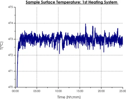
The ﬁnal result was a temperature variation with time as it is shown in ﬁgure 3.8

The new control system consists of a compact microprocessor controller with a PID struc-ture and automatic tuning used along with a thyristor, to reduce the HS power. The resultant measurement temperature curve is shown in ﬁgure 3.9.

(37)

00:00 05:00 10:00 15:00 20:00 25:00

470 471 472 473 474 475

T(

ºC

)

Time (hh:mm)

Sample Surface Temperature: 1st Heating System

Figure 3.8: Samples surface temperature curve for the initial heating system; difference of 2°C between the higher and lower point

00:00 05:00 10:00 15:00 20:00 25:00

470 471 472 473 474 475

Sample Surface Temperature: 2nd Heating System

Time (hh:mm)

T

(º

C

)

Figure 3.9: Samples surface temperature curve for the late heating system; difference of approx-imately 2,5°C between the higher and lower point

(38)

3.1.4 Measuring Components

Temperature Sensors

The temperatures sensors used were platinum resistance thermometers (PRT) more speciﬁcally PT100 (at 0ºC they exhibit a 100Ωresistance) that oﬀer excellent performance in the

tempera-ture range from -200 to +850 °C.

The sensors are made from platinum due to its linear resistance-temperature relationship and its chemical inertness. The platinum wire is encapsulated in a sheath and connected to two copper wires. The copper wires are kept from contacting by a non vacuum stable ceramic insulator. Out-side the sheath this isolation is maintained by a ﬁberglass cover and ceramic cylinders. Whenever the two wires contact the sensor stops working and the system displays a value of T=850. This happened during the course of this work but in most cases only in the experimental working range.

The temperature sensors were first positioned in 8 different locations (see figure 3.6): 2 sensors in the welding seals, 2 in the central part of the radiation shield and 6 in the sample. From these, 4 (in red) were used to control the heating system: 2 at the middle and the remaining 2 in each outer heating zone. To assure its contact with the surface of the sample, the sensors were attached to high temperature resistant coils made of Inconel.

In the new set up the heating parts control was performed separately by one sensor distanced 10 mm from the sample and positioned in the middle of each heating part. Additionally one sensor was wired to the sample to allow the registry and detection of irregular temperature conditions.

Mass Spectrometer

Ion optics

Formation space Filament

(U+Vcosωτ) z

x y

Ion generation by electron collision ionization

in the ion source

Ion separation according to the m/e ratio in the rod system

Ion detection in the ion detector

Figure 3.10: Functioning Principle of QMS 200 [45]; ions with a particu-lar mass/charge ratio are lead by a high electric quadropole field to the ion detector

Initially all the measurements were performed by a quadrupol mass spectrometer Pfeiffer QMS 200. This device is equipped with a 4 parallel metal rod system (figure 3.10), that creates a high frequency electric quadrupol field with a voltage Vcosωτ, a superimposed direct voltage U and radius r0.

The neutral particles arriving in the ionizing space are ionized by the ﬁlaments of the ion source. The ion source is usually protected by a full range gauge that shuts it down in case a pressure higher than1_×10−4 mbar is reached.

(39)

be obtained by varying the frequency (m/e_≈1/ω2_{) or voltage (m/e}

≈V).

In this work the measurement type used was the multiple ion detection (MID) mode. The measured intensities were displayed as a function of time as it is shown in ﬁgure 3.11.

0 10 20 30 40 50

0,0 2,0x10-9 4,0x10-9 6,0x10-9 8,0x10-9 1,0x10-8 1,2x10-8 Permeation measurement: t=25 hours

Current Pressure time (h) C u rr e n t (A )

Initial puming stage t=20 hours

Introduction of H₂

0,0 2,0x10-6 4,0x10-6 6,0x10-6 8,0x10-6 1,0x10-5 Baseline t=5 hours P re ss u re ( m b a r)

Figure 3.11: QMS measurement profile; Current (red) and Pressure (blue) curves, and stage identification

The calibration of the device previous to the experiment is necessary to convert the obtained values of current into gas amount.

The calibration method used in the former work [46] consisted in measuring the ﬂow that passed through a removable capillary with known diameter and length, and compare it to the obtained current.

First the pressure growth rate (mbar/s) was measured: hydrogen was fed into the capillary that led the gas into a closed chamber (in HV) with a known volume. The pressure increase was registered and the flow obtained through the slope of the pressure vs time line. The capillary was then placed between the gas supply and a special sample, with two holes in the ends, in the PMD. After obtaining the baseline, the gas was lead to the holes of the sample and finally pumped by the QMS. After obtaining a constant current, the supply was interrupted and the procedure repeated several times for each capillar. The conversion of current into flow and current was made through the linear regression of the flow vs current graphic.

Due to the degradation of the capillaries used and the impossibility of applying this method at the beginning of each experiment, calibration test leaks, to be attached directly to the QMS, were ordered.

(40)

then proceed but now recurring to pressure measurements.

Pressure Gauges

Two types of pressure gauges were used: a capacitance diaphragm and full range gauge. Capacitance diaphragm gauges are used from atmospheric pressure to 0,1 Pa.

The pressure is measured through the change in capacitance of a plate capacitor constituted by two electrodes: one fixed and the diaphragm. When the diaphragm deflects, due to the variation of pressure, the distance between the two electrodes changes and the capacitance is altered. To ensure sufficient deflection at different pressure levels, diaphragms of several thicknesses are used. In this work capacitance gauges CMR 261 from Pfeiffer, with 0,2% accuracy, measured the input pressure of hydrogen.

Adjacent Electrode

Diaphragm

inlet Pressure distance

Figure 3.12: Diaphragm capacitive

gauges working principle; the inlet pres-sure causes the deflection of the di-aphragm and the capacitance of the sys-tem is altered

The full range gauge consists of Pirani and cold cathode measurement systems combined in such a way to present an uniform behaviour.

In a Pirani system (ﬁgure 3.13), the pressure is measured through the heat loss of a suspended

To Vacuum

Figure 3.13: Pirani Circuit [47]; collision of particles with a metal filament result on the variation of its electrical resistance

metal ﬁlament, result of the collision of gas molecules. If the gas pressure decreases, the num-ber of molecules present will fall proportionately and the wire temperature increases due to the reduced cooling eﬀect. This increase will then result on the variation of the electrical resistance of the wire. In many systems the pressure can also be determined by the measurement of the required current to maintain the wire at a constant temperature.

At pressures lower than 1 Pa the Pirani system can no longer measure and the cold cathode measurement circuit is activated.

(41)

Cathode Plate

Possible electron trajectory Cathode Plate

Magnetic Field

Anode Loop

Figure 3.14: Penning Gauge [47]; electrons confined in a spiral path ionize gas particles that are directed to the cor-responding electrode

for measuring ranges below 1 Pa. Above this level the discharge changes to a glow discharge with intense light output in which the current (at constant voltage) is scarcely dependent on the pressure.

This type of system presents three outstanding advantages: is the least expensive, insensitive to sudden admission of air and vibrations and easy to operate. The big disadvantages are its high susceptibility to contamination, resultant either from the sputtering of the cathode material by the ions produced in the discharge and the continuous operation in the range of 10−2- 1 Pa.

The full range gauges used were Pfeiﬀer PKR 261 models which present reproducibility and accuracy of respectively 5 and 30% of the measured value in the range1_×10−6

-1_×104 _Pa.

3.2 Problems Faced and Respective Resolution

Most significant problems that occurred in the course of this work are displayed in the cause effect diagram of figure 3.15.

The green items represent problems that were permanently resolved. The remaining are situations that were minimized but may again occur.

Observing the diagram one can state that the biggest achievements were a reliable heating system and a reproducible temperature control. The development of the sample preparation procedure also allowed to resolve several experimental errors. In the remaining categories the encountered problems were temporarily resolved and detection methods (such as the use of extra pressure gauges) were enabled.

3.2.1 Heating System

A situation that occurred frequently in the initial PMD was the conduction of current between the heating wire and the HS metallic components (radiation shield and metallic skeleton). This would happen during the experiment and resulted in the shut down of the PMD by the safety fuse. These short circuits were attributed to the heating wire expansion and/or vibration which would then contact the metallic clammers and radiation shield. Tracking these contact points was extremely diﬃcult (sometimes even required the radiation shield to be saw) and the solution, consisting of the placement of ceramic parts, was temporary since they were soon displaced due to heating wire’s expansion/vibration.

(42)

C h a p te r 3 . M a te ria ls a n d M et h o d s 3 1 Defective material Vacuum Components Breakdown Wrong characteristics Turbo Pumps Oil backdiffusion Rotary Vane Pumps Cu seal ductility Flanges Feedthroughs fragility Temperature Regulation Control and Data Recording

Control Dependent on

program response time

Not reliable: sudden deregulation of T for no apparent reason

Labview Regulation Time consuming process Difficult to perform with high

power HS Different

parameters for different chambers

Recording

Corrupted files by the simultaneous use of 2 recording programs (1 for T and other for P) Tiristor

Switched wiring in pins

Control sensors

1 control sensor: temperature profile not reproducible Positioning in sample Difficult to reproduce Difficult to assure Heating System Insufficient isolation not replaceable Ceramic rings Fixed Radiation shields Relative position with the heating wire Stress points Heating wire Sample

Leak in the Swagelok connection Sample not straight QMS Not calibrated Possible contamination of

the ion detector Pressure

Gauges Influence of the magnetic field in HS and QMS behaviour

Circuit wouldn't change from Piranni to Penning mode

Contamination of the cathode

Temperature sensors

Deterioration of the ceramic insulator

Measuring Components

Problems Faced

(43)

With the new heating system short circuits may occasionally occur but due to the isolation provided by the glass covering, the amount of possible contact points was strongly reduced. The few remaining can be easily detected and prevented since the radiation shield is easily removable.

3.2.2 Temperature Regulation, Control and Data Recording

LabView Limitations

The temperature control and recording was initially performed exclusively by a LabView in-terface. This software for simple procedures is quite good, however its use revealed not to be advisable for a simultaneous automated control of at least 4 temperatures. The program used was heavy and its performance could be aﬀected by a change in the computers CPU utilization. This might explain the sudden temperature deregulation detected more than once.

The tuning of the automate parameters was painfully achieved for one heating system. Nonethe-less this process was not only time consuming but had to be repeated every time the measurement temperature would change.

With the microprocessor controller the tuning was automatic and only one situation of tempera-ture deregulation was observed. Since there was no obscure software in between, soon the source (switched wiring in the thyristor) was found.

A LabView program is currently used only to register the temperature and pressure data.

Number of Sensors and Positioning

The higher level of reproducibility within trials was also achieved by the deﬁnition of the optimal position and number of the controlling sensors.

The temperature control at the surface of the sample was initially guaranteed with the assistance of Inconel coils which assured the sensors positioning. However with the introduction of the sample, the coils would deteriorate and after a few runs was no longer possible to control the sensors position and subsequently the temperature proﬁle in the experiment. The use of the coils was then discarded and in the new HS the control sensors were wired at the surface of the sample. Yet after the sample has been removed of the chamber, it would be often veriﬁed that the sensor positioning would have changed. It was not possible to know if this had occurred in introduction, withdraw or during the experiment as a consequence of expansion of the connecting wire. To minimize the temperature variation within the several trials, the control should be performed in such position that wouldn’t vary with the samples introduction/removal. The sensors were then positioned 10 mm away from the sample.

The need to simplify the control of the heating system and the observation of some situations where the sensors had stopped working lead to the reduction of the number of control sensors initially used (4). First only one sensor positioned between the two heating parts was used to control the second HS. However the two registry sensors positioned in the sample indicated that the two heating parts would behave differently from one trial to another (see figure 3.16). For this reason the two heating parts were ultimately controlled separately by one sensor at their middle position (see sensor relative positioning in figures 3.22 and 3.23).

3.2.3 Sample