ACPD
13, 15697–15747, 2013N2O emissions 1999–2009 from a global atmospheric
inversion
R. L. Thompson et al.
Title Page
Abstract Introduction
Conclusions References
Tables Figures
◭ ◮
◭ ◮
Back Close
Full Screen / Esc
Printer-friendly Version Interactive Discussion
Discussion
P
a
per
|
Di
scussion
P
a
per
|
Discussion
P
a
per
|
Discussi
on
P
a
per
|
Atmos. Chem. Phys. Discuss., 13, 15697–15747, 2013 www.atmos-chem-phys-discuss.net/13/15697/2013/ doi:10.5194/acpd-13-15697-2013
© Author(s) 2013. CC Attribution 3.0 License.
Atmospheric Chemistry and Physics
Open Access
Discussions
Geoscientiic Geoscientiic
Geoscientiic Geoscientiic
This discussion paper is/has been under review for the journal Atmospheric Chemistry and Physics (ACP). Please refer to the corresponding final paper in ACP if available.
Nitrous oxide emissions 1999–2009 from
a global atmospheric inversion
R. L. Thompson1, F. Chevallier2, A. M. Crotwell3,10, G. Dutton3,
R. L. Langenfelds4, R. G. Prinn5, R. F. Weiss6, Y. Tohjima7, T. Nakazawa8,
P. B. Krummel4, L. P. Steele4, P. Fraser4, K. Ishijima9, and S. Aoki8
1
National Institute for Air Research, Kjeller, Norway
2
Laboratoire des Sciences du Climat et de l’Environnement, Gif sur Yvette, France
3
NOAA ESRL, Global Monitoring Division, Boulder, CO, USA
4
Commonwealth Scientific and Industrial Research Organisation, Aspendale, Australia
5
Center for Global Change Science, MIT, Cambridge, MA, USA
6
Scripps Institution of Oceanography, La Jolla, CA, USA
7
National Institute for Environmental Studies, Tsukuba, Japan
8
Tohoku University, Sendai, Japan
9
Japan Agency for Marine-Earth Science and Technology, Yokohama, Japan
10
ACPD
13, 15697–15747, 2013N2O emissions 1999–2009 from a global atmospheric
inversion
R. L. Thompson et al.
Title Page
Abstract Introduction
Conclusions References
Tables Figures
◭ ◮
◭ ◮
Back Close
Full Screen / Esc
Printer-friendly Version Interactive Discussion
Discussion
P
a
per
|
Di
scussion
P
a
per
|
Discussion
P
a
per
|
Discussi
on
P
a
per
|
Received: 22 March 2013 – Accepted: 28 May 2013 – Published: 13 June 2013 Correspondence to: R. L. Thompson ([email protected])
ACPD
13, 15697–15747, 2013N2O emissions 1999–2009 from a global atmospheric
inversion
R. L. Thompson et al.
Title Page
Abstract Introduction
Conclusions References
Tables Figures
◭ ◮
◭ ◮
Back Close
Full Screen / Esc
Printer-friendly Version Interactive Discussion
Discussion
P
a
per
|
Di
scussion
P
a
per
|
Discussion
P
a
per
|
Discussi
on
P
a
per
|
Abstract
N2O surface fluxes were estimated for 1999 to 2009 using a time-dependent Bayesian inversion technique. Observations were drawn from 5 different networks, incorporating 59 surface sites and a number of ship-based measurement series. To avoid biases in the inverted fluxes, the data were adjusted to a common scale and scale offsets were
5
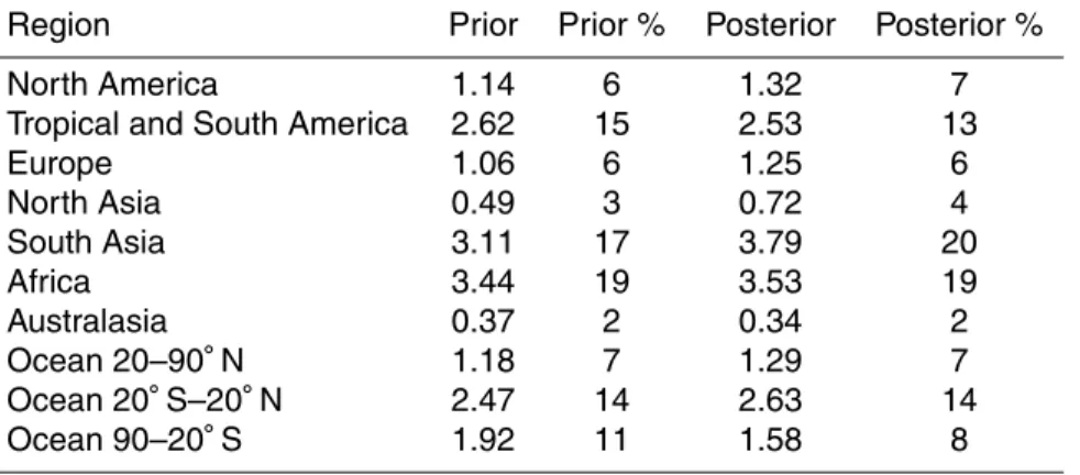
included in the optimization problem. The fluxes were calculated at the same resolution as the transport model (3.75◦longitude×2.5◦latitude) and at monthly time resolution. Over the 11 yr period, the global total N2O source varied from 17.5 to 20.1 Tg a−1 N. Tropical and subtropical land regions were found to consistently have the highest N2O emissions, in particular, in South Asia (20 % of global total), South America (13 %) and
10
Africa (19 %), while emissions from temperate regions were smaller, Europe (6 %) and North America (7 %). A significant multi-annual trend in N2O emissions (0.045 Tg a−2 N) from South Asia was found and confirms inventory estimates of this trend. Consid-erable inter-annual variability in the global N2O source was observed (0.8 Tg a−1 N, 1 standard deviation, SD) and was largely driven by variability in tropical and subtropical
15
soil fluxes, in particular in South America (0.3 Tg a−1 N, 1 SD) and to a lesser extent in Africa (0.3 Tg a−1 N, 1 SD). Notable variability was also found for N2O fluxes in the tropical and southern oceans (0.15 and 0.2 Tg a−1N, 1 SD, respectively). Inter-annual variability in the N2O source correlates strongly with ENSO, where El Niño conditions are associated with lower N2O fluxes from soils and from the ocean and vice-versa for
20
La Niña conditions.
1 Introduction
Nitrous oxide (N2O) is now considered to be the third most important long-lived anthro-pogenic greenhouse gas (GHG) and has a global warming potential of approximately 300 times that of CO2(Forster et al., 2007). N2O also plays an important role in
strato-25
chlo-ACPD
13, 15697–15747, 2013N2O emissions 1999–2009 from a global atmospheric
inversion
R. L. Thompson et al.
Title Page
Abstract Introduction
Conclusions References
Tables Figures
◭ ◮
◭ ◮
Back Close
Full Screen / Esc
Printer-friendly Version Interactive Discussion
Discussion
P
a
per
|
Di
scussion
P
a
per
|
Discussion
P
a
per
|
Discussi
on
P
a
per
|
rofluorocarbon (CFC) emissions, is the dominant ozone depleting substance currently emitted (Ravishankara et al., 2009). Emissions of N2O have been increasing since the pre-industrial era due to human activities leading to substantial increases in the atmo-spheric mole fraction, from 270 nmol mol−1(abbreviated as ppb, 1 nmol=10−9mol) to around 323 ppb today (WMO, 2011). N2O emissions occur naturally as a byproduct
5
of the processes of denitrification (microbial reduction of nitrate and nitrite) and nitri-fication (microbial oxidation of ammonia), which occur in soils and in the ocean. Sev-eral human activities enhance nitrification and denitrification rates and, consequently, emissions of N2O to the atmosphere. The most significant of these activities is food production through the use of nitrogen fertilizers, manure, and land cultivation (Syakila
10
and Kroeze, 2011), with lesser contributions from bio-fuel production (Crutzen et al., 2008). There are also direct N2O emissions from industry, combustion and municipal waste (Denman et al., 2007).
Atmospheric monitoring of N2O started in the late 1970s and has been instrumen-tal in determining long-term emission trends (Syakila and Kroeze, 2011), and more
15
recently with improved data precision, in determining the spatial distribution of emis-sions (Hirsch et al., 2006; Huang et al., 2008). Super-imposed on the long-term trend in atmospheric N2O, is considerable inter-annual variability in the growth rate. To date, there have been only a few studies that have tried to understand the mechanisms driving this variability (Nevison et al., 2011, 2007). On one hand, the growth rate is
20
influenced by changes in non-flux related variables, such as atmospheric transport in-cluding stratosphere to troposphere transport, which carries N2O-depleted air from the stratosphere into the troposphere and has a significant influence on the observed N2O seasonal cycle and contributes also to inter-annual variability (Nevison et al., 2011). On the other hand, it is known from in-situ flux measurements that terrestrial biosphere
25
ACPD
13, 15697–15747, 2013N2O emissions 1999–2009 from a global atmospheric
inversion
R. L. Thompson et al.
Title Page
Abstract Introduction
Conclusions References
Tables Figures
◭ ◮
◭ ◮
Back Close
Full Screen / Esc
Printer-friendly Version Interactive Discussion
Discussion
P
a
per
|
Di
scussion
P
a
per
|
Discussion
P
a
per
|
Discussi
on
P
a
per
|
response of N2O production to soil and climate parameters, as well as to nitrogen sub-strate availability, the modelled fluxes are associated with large uncertainties (Werner et al., 2007). Some ecosystem models predict a significant N2O soil flux–climate link. In a study by Xu-Ri et al. (2012) soil temperature increases alone resulted in a 1 Tg of N equivalents of N2O (abbreviated Tg N) increase in soil emission in the 20th century.
5
A study by Zaehle et al. (2011) also found a strong link between N2O soil emissions and climate. It has not been possible, however, to verify modelled inter-annual variabil-ity in the N2O flux since sufficient long-term in-situ flux measurements are not available. Therefore, to learn more about inter-annual variability in N2O fluxes and, especially the integrated response at regional or continental scales of N2O flux to climate forcing, it is
10
useful to turn to atmospheric observations.
Numerous multi-annual flux studies have been made for the other important GHGs: CO2 (Bousquet et al., 2000; Rayner et al., 1999; Rödenbeck et al., 2003) and CH4 (Bousquet et al., 2006) using atmospheric observations and the inversion of atmo-spheric transport. These flux studies found the land-atmosphere fluxes of both these
15
species to be significantly sensitive to climate variation and, in particular, to the El Niño Southern Oscillation (ENSO) climate variation and to the climate impacts of the Pinatubo eruption (Bousquet et al., 2006; Peylin et al., 2005; Rödenbeck et al., 2003). To the best of the authors’ knowledge, no previous multi-annual inversion study of this type has been made for N2O. In this study, we focus on N2O fluxes from 1999 to
20
2009, since the data precision improved greatly during the 1990s and since a number of new sites became operational in the late 1990s and early 2000s. The inversions were run from 1996 to 2009 but we only examine the data from 1999 since the 3 first years of simulation were needed for spin-up. (The long spin-up time was required to achieve realistic tropospheric and stratospheric mole fractions, which depend on the
25
surface source, the stratospheric sink and the rate of air mass exchange across the tropopause.)
ACPD
13, 15697–15747, 2013N2O emissions 1999–2009 from a global atmospheric
inversion
R. L. Thompson et al.
Title Page
Abstract Introduction
Conclusions References
Tables Figures
◭ ◮
◭ ◮
Back Close
Full Screen / Esc
Printer-friendly Version Interactive Discussion
Discussion
P
a
per
|
Di
scussion
P
a
per
|
Discussion
P
a
per
|
Discussi
on
P
a
per
|
(Sect. 2). Secondly, we describe a number of tests that were made for the sensitivity of the observation network to changes in N2O emissions and for the sensitivity of the in-versions to their prior emission estimates (Sects. 2.6 and 2.7, respectively). In Sects. 3 and 4, we discuss the results of the inversions and the variability and trends in the retrieved N2O emissions.
5
2 Inversion method
2.1 Bayesian inversion
In this study, we used the Bayesian inversion method to find the optimal surface fluxes at monthly temporal resolution and at the same spatial resolution as the atmospheric transport model (i.e. 3.75◦×2.5◦ longitude by latitude). The inversion is performed in
10
two time intervals, from 1996 to 2003 and 2002 to 2009. The first 3 a of the first period and the first 2 a of the second period were used for spin-up. (A 2 a spin-up time was considered sufficient for the second period, since the initial conditions for 2002 from the first period were re-used in the second period.) According to the Bayesian method, the optimal solution (in this study it is the surface fluxes and the initial mole fractions),x, 15
are those that provide the best fit to the atmospheric observations,y, while remaining
within the bounds of the prior estimates,xb, and their uncertainties (for details about
the Bayesian method refer to Tarantola, 2002). The extra constraint of the prior prevents the problem from being ill-conditioned in the mathematical sense. Based on Bayesian theory, and Gaussian-error hypotheses, one can derive the following cost function:
20
J(x)=(x−xb)TB−1(x−xb)+(H(x)−y)TR−1(H(x)−y) (1)
where the flux uncertainties are described by the error covariance matrix,B, the obser-vation uncertainties are described by the error covariance matrix,R, and H is a non-linear operator for atmospheric transport and chemistry (in Eq. 1, the matrix trans-pose is indicated by T). To solve this equation, we used the variational framework of
ACPD
13, 15697–15747, 2013N2O emissions 1999–2009 from a global atmospheric
inversion
R. L. Thompson et al.
Title Page
Abstract Introduction
Conclusions References
Tables Figures
◭ ◮
◭ ◮
Back Close
Full Screen / Esc
Printer-friendly Version Interactive Discussion
Discussion
P
a
per
|
Di
scussion
P
a
per
|
Discussion
P
a
per
|
Discussi
on
P
a
per
|
Chevallier et al. (2005). In this approach, the minimum ofJ(x) is found iteratively using
a descent algorithm based on the Lanczos version of the conjugate gradient algorithm (Lanczos, 1950). This algorithm requires several computations of the gradient ofJwith respect tox(whereHis the linearized form of the transport operator,H):
1/2∇J(x)=B−1(x−xb)+HTR−1(H(x)−y) (2) 5
For problems with a very large number of variables, it is not possible to directly defineHorHT owing to numerical limitations. Therefore, the elements ofHT are found implicitly via the adjoint model of the atmospheric transport and chemistry (Chevallier et al., 2005; Errico, 1997).
2.2 Transport model
10
The inversion framework relies on the off-line version of the Laboratoire de Météorolo-gie Dynamique, version 4 (LMDz) general circulation model (Hourdin and Armengaud, 1999; Hourdin et al., 2006). This version computes the evolution of atmospheric com-pounds using archived fields of winds, convection mass fluxes, and planetary bound-ary layer (PBL) exchange coefficients that have been built from prior integrations of
15
the complete general circulation model, which was nudged to ECMWF ERA-40 winds (Uppala et al., 2005). The LMDz model is on a 3-D Eulerian grid consisting of 96 zonal columns and 73 meridional rows and 19 hybrid pressure levels. The daytime PBL is resolved by 4–5 levels, the first of which corresponds to 70 m, and are spaced between 300 to 500 m apart from there upwards. Above the PBL the mean resolution is 2 km up
20
to a height of 20 km, above which there are 4 levels with the uppermost level at 3 hPa. Tracer transport is calculated in LMDz using the second order finite-volume method of Van Leer (1977) and is described for LMDz by Hourdin and Armengaud (1999). Tur-bulent mixing in the PBL is parameterized using the scheme of Mellor and Yamada (1982) and thermal convection is parameterized according to the scheme of Tiedtke
25
ACPD
13, 15697–15747, 2013N2O emissions 1999–2009 from a global atmospheric
inversion
R. L. Thompson et al.
Title Page
Abstract Introduction
Conclusions References
Tables Figures
◭ ◮
◭ ◮
Back Close
Full Screen / Esc
Printer-friendly Version Interactive Discussion
Discussion
P
a
per
|
Di
scussion
P
a
per
|
Discussion
P
a
per
|
Discussi
on
P
a
per
|
calculation ofJand its gradient∇J (Eqs. 1 and 2), the tangent linearHand adjointHT
operators were coded from the off-line LMDz version (Chevallier et al., 2005).
In the case of N2O, the sink in the stratosphere needs to be accounted for. Losses of N2O occur via photolysis and reaction with O1D accounting for 90 % and 10 % of the sink, respectively (Minschwaner et al., 1993). These reactions were included in the
5
forward and adjoint models of the atmospheric transport as described in Thompson et al. (2011). The number density of O(1D) and the photolysis rate were defined for each grid-cell and time-step and were taken from prior simulations of the coupled global circulation and atmospheric chemistry model LMDz-INCA (Hauglustaine et al., 2004) with the same transport fields as used in the inversion. The fields of photolysis rate
10
from LMDz-INCA were scaled by a factor of 0.66 to give a mean total annual loss of N2O of 12.2 Tg a−1N, consistent with estimates of N2O lifetime between 124 and 130 a (Prather et al., 2012; Volk et al., 1997).
2.3 Prior flux estimates
Our a priori N2O flux estimate (xb in Eqs. 1 and 2) was compiled from different mod-15
els/inventories for:
– terrestrial biosphere fluxes, including natural and cultivated ecosystems
– anthropogenic emissions, from fossil and bio-fuel combustion, industry, and mu-nicipal waste
– biomass burning emissions
20
– coastal and open ocean fluxes
ACPD
13, 15697–15747, 2013N2O emissions 1999–2009 from a global atmospheric
inversion
R. L. Thompson et al.
Title Page
Abstract Introduction
Conclusions References
Tables Figures
◭ ◮
◭ ◮
Back Close
Full Screen / Esc
Printer-friendly Version Interactive Discussion
Discussion
P
a
per
|
Di
scussion
P
a
per
|
Discussion
P
a
per
|
Discussi
on
P
a
per
|
and fertilizer usage and simulates nitrogen losses via leaching, nitrification and den-itrification pathways, and emissions of trace gases to the atmosphere. The model is driven by climate data (CRU-NCEP) and inter-annually varying N inputs. Data were originally provided at 3.75◦×2.5◦(longitude by latitude) and monthly resolution. For the anthropogenic emissions (excluding direct agricultural emissions, which are accounted
5
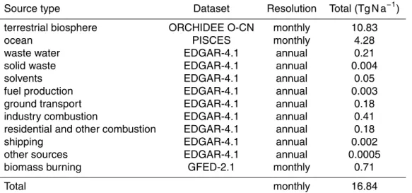
for in O-CN), we used EDGAR-4.1 (Emission Database for Global Atmospheric Re-search) inventory data. These data were provided at 1.0◦×1.0◦ and annual resolution. Since N2O emissions from these sources are small relative to the terrestrial biosphere and ocean sources, and because they have relatively little seasonality, annual reso-lution is considered sufficient. The biomass burning emissions were provided by the
10
Global Fire Emissions Database (GFED-2.1) at 1.0◦×1.0◦and monthly resolution (van der Werf et al., 2010). For the ocean fluxes, we used estimates provided by the ocean biogeochemistry model, PISCES, which was embedded in a climate model but was not constrained by meteorological data, thus inter-annual variations may not be in-phase with observations (Dutreuil et al., 2009). Data were provided at 1.0◦×1.0◦and monthly
15
resolution (see Table 3 for the global N2O emission from each source).
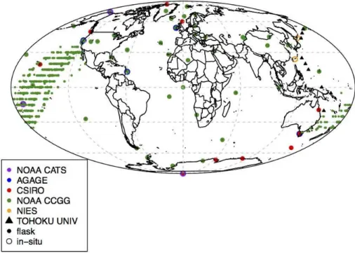
2.4 Observations
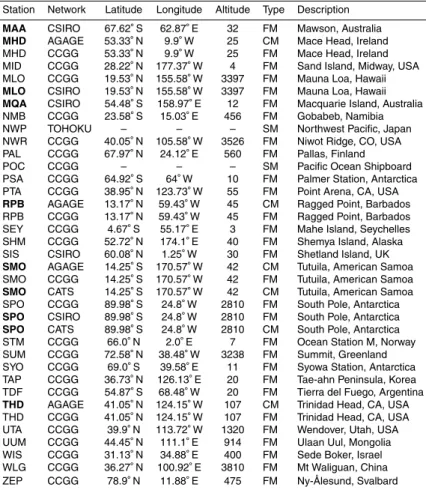
Atmospheric observations were pooled from a number of global networks, indepen-dent sites, and ship-based measurements (see Figs. 1 and 2 and Table 1). Long-term records of N2O mole fraction are available from the Advanced Global Atmospheric
20
Gases Experiment (AGAGE, http://cdiac.ornl.gov/ftp/ale_gage_Agage/AGAGE/) and the NOAA Halocarbons and other Atmospheric Trace Species (HATS, http://www. esrl.noaa.gov/gmd/hats/), including both the OTTO and the Chromatograph for At-mospheric Trace Species (CATS, http://www.esrl.noaa.gov/gmd/hats/insitu/cats/) pro-grammes, which were established in the 1990s. The early data, however, cannot be
25
ACPD
13, 15697–15747, 2013N2O emissions 1999–2009 from a global atmospheric
inversion
R. L. Thompson et al.
Title Page
Abstract Introduction
Conclusions References
Tables Figures
◭ ◮
◭ ◮
Back Close
Full Screen / Esc
Printer-friendly Version Interactive Discussion
Discussion
P
a
per
|
Di
scussion
P
a
per
|
Discussion
P
a
per
|
Discussi
on
P
a
per
|
from the mid to late 1990s. Both the AGAGE and CATS networks consist of stations equipped with in-situ Gas Chromatographs and Electron Capture Detectors (GC-ECD) to measure the dry air mole fraction of N2O (nmol mol−1, abbreviated as ppb) and pro-vide measurements at approximately 40 min intervals. The AGAGE data are reported on the SIO1998 scale and have an uncertainty on individual measurements of about
5
0.1 ppb (Prinn et al., 2000) while the NOAA CATS data are reported on the NOAA2006 scale and have an uncertainty of about 0.3 ppb (Hall et al., 2007). In the late 1990s and early 2000s, NOAA also established a flask network under the Carbon Cycle and Greenhouse Gases (CCGG, http://www.esrl.noaa.gov/gmd/ccgg/) programme. Flask samples from this network are also analyzed by GC-ECD in a central laboratory and
10
are reported on the NOAA2006A scale. These data have an uncertainty of 0.4 ppb based on the mean value of differences from paired flasks. There is some concern that there could be a calibration shift between NOAA CCGG data collected before and after 2001, owing to a poor calibration routine used prior to 2001. To test for the influ-ence of this shift on the retrieved fluxes, we include an inversion test in which minimal
15
NOAA CCGG data is included (test IAVR, see Sect. 2.7 for details). The Common-wealth Scientific and Industrial Research Organisation (CSIRO) in Australia also oper-ate a flask network since the early 1990s (data available from the World Data Centre for Greenhouse Gases: http://ds.data.jma.go.jp/gmd/wdcgg/). These measurements are reported on the NOAA2006 scale with an uncertainty of approximately 0.3 ppb for each
20
flask measurement (Francey et al., 2003). In addition, we included data from two sta-tions operated by the National Institute for Environmental Science (NIES) in Japan, which operate in-situ GC-ECDs (data are available on request to NIES). These data are reported on NIES’s own scale, which is approximately 0.6 ppb lower than NOAA2006 for ambient concentrations (Y. Tohjima, personal communication, 2012). Lastly, we
in-25
ACPD
13, 15697–15747, 2013N2O emissions 1999–2009 from a global atmospheric
inversion
R. L. Thompson et al.
Title Page
Abstract Introduction
Conclusions References
Tables Figures
◭ ◮
◭ ◮
Back Close
Full Screen / Esc
Printer-friendly Version Interactive Discussion
Discussion
P
a
per
|
Di
scussion
P
a
per
|
Discussion
P
a
per
|
Discussi
on
P
a
per
|
approximately 0.2 ppb higher than the NOAA2006A scale (for a list of all stations and their locations, see Table 1).
Gradients of N2O mole fraction in the atmosphere, which provide information about the distribution of N2O fluxes, can be small and of the same order of magnitude as the calibration offsets between different scales and networks. For this reason, it is of
5
critical importance to correct for these offsets prior to and/or in the inversion. Corazza et al. (2011) incorporated the optimization of calibration offsets into their inversion prob-lem, thereby reducing the bias that these have on the retrieved fluxes. We adopt the same approach as Corazza et al. (2011) but, in addition, we corrected the observations based on our prior estimated calibration offsets before running the inversion. Using
10
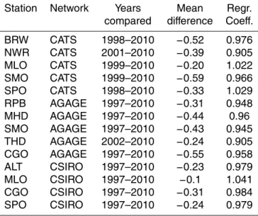
both approaches means that the inversion will only “fine-tune” the offsets thereby limit-ing the degrees of freedom that can be used for this adjustment. Prior calibration offsets were estimated relative to NOAA CCGG (NOAA2006A scale) based on the compari-son of observations from two or more networks at the same location, e.g. in American Samoa, where NOAA CATS, NOAA CCGG and AGAGE all have measurements.
Over-15
laps between NOAA CCGG and AGAGE also exist at MHD, CGO, RPB, and THD, and between NOAA CCGG and CSIRO at ALT, MLO, CGO, and SPO, where the data were corrected to the NOAA2006A scale using the linear trend and offset calculated at each site (see Table 2). At sites where there was no overlap, the mean of the corrections applied to other sites within the same network was used. For NIES, which has no
over-20
lap with other networks, a temporally fixed offset was used and was based on shared cylinder inter-comparisons with NOAA CCGG (Y. Tohjima, personal communication, 2012). The comparisons of AGAGE and NOAA CCGG data show a significant trend in the offset (0.02–0.04 ppb a−1), which is consistent at all compared sites and points to a possible calibration drift in the scales relative to each other. However, without further
25
ACPD
13, 15697–15747, 2013N2O emissions 1999–2009 from a global atmospheric
inversion
R. L. Thompson et al.
Title Page
Abstract Introduction
Conclusions References
Tables Figures
◭ ◮
◭ ◮
Back Close
Full Screen / Esc
Printer-friendly Version Interactive Discussion
Discussion
P
a
per
|
Di
scussion
P
a
per
|
Discussion
P
a
per
|
Discussi
on
P
a
per
|
All data were filtered for suspicious values using flags set by the data providers. Additionally, the data were filtered for outliers, which were defined as points outside 2 SD of the running mean calculated over a window of 45 days for flask data and 3 days for in-situ data. The window lengths were optimized on a trial basis to ensure that only suspicious values were removed.
5
Observations from sites with in-situ GC-ECDs were selected for the afternoon (12:00 to 17:00 LT) if they were low altitude sites (<1000 m a.s.l.) and for the night (00:00 to 06:00 LT) if they were mountain sites (>1000 m a.s.l.). These data selection crite-ria were chosen to minimise the impact of transport model errors. In general, data were assimilated at hourly resolution. For flask data, no selection was applied and data
10
were assimilated when available. For the ship-based data (from Tohoku University), one observation was assimilated per grid-cell and time-step and where more than one observation was available the values were averaged. This was done to avoid assimi-lating highly correlated observations (observation error correlations are not taken into account, see Sect. 2.5.2).
15
2.5 Specification of uncertainties
2.5.1 Prior flux error covariance matrix
A key aspect of the Bayesian inversion is the description of prior flux uncertainty. This uncertainty is described by the error covariance matrix,B (in Eqs. 1 and 2), in which the diagonal elements are the error variances in each grid-cell and time-step and the
20
off-diagonal elements are the covariances. Unfortunately, there are insufficient obser-vations of N2O flux to be able to accurately determine the error variances and covari-ances. Therefore, a simple approach for this was used, i.e. we calculated the variance of each land grid-cell as the maximum flux for the year found in the 8 surrounding grid cells plus the cell of interest. Choosing the maximum value from 9 grid cells allows the
25
ACPD
13, 15697–15747, 2013N2O emissions 1999–2009 from a global atmospheric
inversion
R. L. Thompson et al.
Title Page
Abstract Introduction
Conclusions References
Tables Figures
◭ ◮
◭ ◮
Back Close
Full Screen / Esc
Printer-friendly Version Interactive Discussion
Discussion
P
a
per
|
Di
scussion
P
a
per
|
Discussion
P
a
per
|
Discussi
on
P
a
per
|
land approach to avoid overestimating the errors in ocean grid-cells along coastlines. The errors calculated for land in the Southern Hemisphere were scaled by 0.66 ow-ing to the weaker observational constraint in this hemisphere and, therefore, to allow greater reliance on the prior estimates. Both land and ocean errors were set to a maxi-mum of 0.44 g N m−2a−1and minimum of 0.03 g N m−2a−1. In areas covered by sea-ice,
5
the error was reduced by a factor of 100. The covariance was calculated as an expo-nential decay with distance and time using correlation scale lengths of 500 km over land and 1000 km over ocean, and 12 weeks, respectively. The correlation scale length of the errors in land fluxes depends strongly on the source; here we chose 500 km as an educated guess to represent the correlation of the errors in the spatially diffuse
10
soil emission, which is the dominant source and is modulated by land-use, soil type, moisture and temperature, as well as by the amount of nitrogen input. The whole error covariance matrix was then scaled so that its sum was consistent with an assumed global total prior uncertainty of 2 Tg a−1N.
2.5.2 Observation error covariance matrix
15
Another key component of the Bayesian inversion is the observation uncertainty, which is described by the error covariance matrix,R. A thorough description of the observa-tion error variances is needed to avoid giving too strong weighting to very uncertain observations, which becomes particularly important if these observations are far from the expected value. The observation error variance takes into account the
measure-20
ment and transport model errors. Measurement errors consist of random and system-atic components. Random errors are assessed in determining the measurement re-producibility, while systematic errors, such as errors in the calibration, instrumentation, air sampling, etc are more difficult to determine. For the measurement error, we have used the estimates given by the data providers, which includes random and, as far as
25
ACPD
13, 15697–15747, 2013N2O emissions 1999–2009 from a global atmospheric
inversion
R. L. Thompson et al.
Title Page
Abstract Introduction
Conclusions References
Tables Figures
◭ ◮
◭ ◮
Back Close
Full Screen / Esc
Printer-friendly Version Interactive Discussion
Discussion
P
a
per
|
Di
scussion
P
a
per
|
Discussion
P
a
per
|
Discussi
on
P
a
per
|
Bergamaschi et al., 2010), both of which were calculated using forward model simula-tions run with the same prior fluxes and meteorology as the inversions. The first error uses the 3-D mole fraction gradient around the grid-cell where the site is located as a proxy for the transport error, so that strong vertical and/or horizontal gradients lead to large error estimates. The second error uses the change in mole fraction in the
grid-5
cell integrated over the e-folding time for flushing the grid-cell with the modelled wind speed. This is used as a proxy for the influence of not accounting for the homogeneous distribution of fluxes within the grid-cell and their location relative to the observation site (for details see Bergamaschi et al., 2010). For observations from southern mid to high latitude sites, we have included an additional transport error to account for the fact that
10
LMDz cannot accurately reproduce the seasonal cycle at these latitudes owing largely to errors in Southern Hemisphere stratosphere to troposphere transport (unpublished work). This error was estimated to be approximately 1.0 ppb. We did not account for correlations between errors, i.e.Ris a diagonal matrix.
2.6 Forward model sensitivity tests
15
One major motivation of this study is to determine whether or not N2O emissions vary inter-annually on a regional scale, driven, for example, by ENSO climate variation. It is, therefore, important to first ascertain if such a flux signal can be detected by the current observational network. Since ENSO largely affects the tropics, in particular Tropical and South America, we focus on a hypothetical flux signal from this region. We performed
20
forward model simulations to test the influence of low/high fluxes during one year in tropical and subtropical South America (1 Tg a−1 N less/more evenly distributed over land than in the prior) on atmospheric N2O mole fractions in an El Niño year (1998) and a La Niña year (1999), respectively (the results of these tests are presented in Sect. 3.1).
ACPD
13, 15697–15747, 2013N2O emissions 1999–2009 from a global atmospheric
inversion
R. L. Thompson et al.
Title Page
Abstract Introduction
Conclusions References
Tables Figures
◭ ◮
◭ ◮
Back Close
Full Screen / Esc
Printer-friendly Version Interactive Discussion
Discussion
P
a
per
|
Di
scussion
P
a
per
|
Discussion
P
a
per
|
Discussi
on
P
a
per
|
2.7 Inversion sensitivity tests
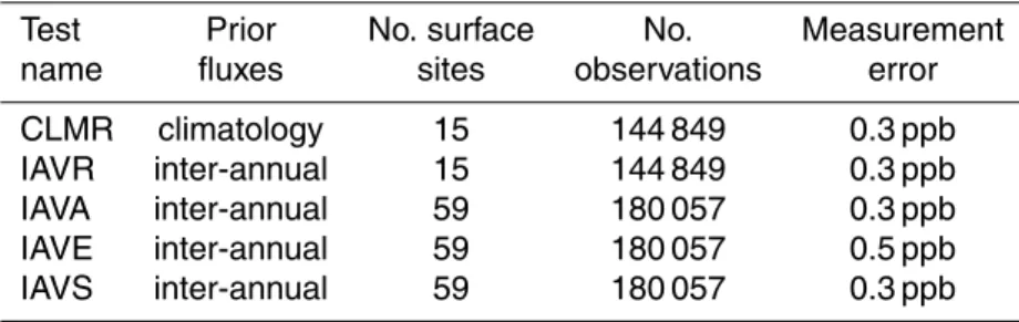
We ran five different inversion scenarios to test the robustness of the results to the observations used and to the inversion set-up (see Table 4). Observation data contains gaps, in other words the data coverage is not consistent throughout the inversion period (see Fig. 2). Furthermore, some observation sites only became operational a few years
5
after the start year of the inversion. The inconsistent data coverage over time results in varying degrees of constraint on the fluxes in space and time, so that in periods with good data coverage a stronger constraint on the fluxes is possible whereas when there is poorer data coverage, the fluxes are closer to the prior. Hence, to examine inter-annual variations in the fluxes, it is necessary to distinguish between variations
10
owing to inconsistent data coverage and those resulting from the atmospheric signal. We, therefore, ran a set of inversions with as consistent as possible data coverage (the reference dataset) and a set of inversions using all available observation sites. For the reference dataset inversions, 15 sites were included, which had data throughout the inversion period and no gaps of longer than 6 months while for the other inversions, 59
15
sites were included and no gap criterion was applied (see Table 1 for the list of sites). The reference dataset inversions also serve as a test for the influence of a potential NOAA CCGG scale shift (see Sect. 2.4) as only one NOAA CCGG site was included in this dataset. The reference dataset inversions consisted of one run using the inter-annually varying prior fluxes (IAVR) and one run with climatological prior fluxes (CLMR)
20
to test the influence of the assumed flux inter-annual variability. For the CLMR run, one year of fluxes (2002) was repeated for every year. The other set of inversions (using all data) were made with inter-annually varying fluxes and consisted of one run to test the sensitivity of the results to the observation error (IAVE), one test where the stratospheric sink was also included in the optimization (IAVS) according to the
25
ACPD
13, 15697–15747, 2013N2O emissions 1999–2009 from a global atmospheric
inversion
R. L. Thompson et al.
Title Page
Abstract Introduction
Conclusions References
Tables Figures
◭ ◮
◭ ◮
Back Close
Full Screen / Esc
Printer-friendly Version Interactive Discussion
Discussion
P
a
per
|
Di
scussion
P
a
per
|
Discussion
P
a
per
|
Discussi
on
P
a
per
|
2.8 Calculation of posterior flux errors
From the Lanczos algorithm used to find the gradient ofJ(x), we also obtain an
esti-mate of the leading eigenvectors of the Hessian matrixJ′′(x). The number of
eigenvec-tors obtained equals the number of iterations performed. This fact is particularly useful since the inverse ofJ′′(x) gives the posterior flux error covariance matrix,A. However, 5
since the eigenvalues of J′′(x) are the reciprocals of the eigenvalues of A, many
it-erations are needed to obtain sufficient eigenvalues and eigenvectors to approximate
A (Chevallier et al., 2005). Therefore, we use the Monte Carlo approach instead to estimate the posterior flux errors as described by Chevallier et al. (2007). In this ap-proach, an ensemble of inversions is run with random perturbations in the prior fluxes
10
and observations, consistent withBandR, respectively. The statistics of the ensemble of posterior fluxes is equivalent to the posterior uncertainty. For the uncertainty cal-culation we used an ensemble of 20 inversions of one year (2003) for the reference and full observation datasets. The prior and posterior uncertainties given in Table 5 are calculated all calculated from the Monte Carlo ensemble.
15
3 Results
3.1 Robustness and uncertainty analysis
The current observational network has few sites in tropical regions and, in particular, no sites in tropical and subtropical South America. However, some constraint on fluxes in this region is obtained from sites in the South Atlantic and Equatorial Pacific. From the
20
forward sensitivity tests, significant differences in atmospheric mole fractions at tropi-cal and subtropitropi-cal sites were found after 2–3 months and globally after circa 6 months following the perturbation. Figure 3 shows the difference in mole fraction (test scenario minus control run) at Samoa and Ascension Island for an El Niño year (low fluxes) and a La Niña year (high fluxes). The current measurement precision on a single flask
ACPD
13, 15697–15747, 2013N2O emissions 1999–2009 from a global atmospheric
inversion
R. L. Thompson et al.
Title Page
Abstract Introduction
Conclusions References
Tables Figures
◭ ◮
◭ ◮
Back Close
Full Screen / Esc
Printer-friendly Version Interactive Discussion
Discussion
P
a
per
|
Di
scussion
P
a
per
|
Discussion
P
a
per
|
Discussi
on
P
a
per
|
ple is approximately 0.3 ppb, so the signal after approximately 6 months (circa 0.2 ppb) will be detectable from the mean of 4 or more flask samples. If the change in flux persists for the order of 1 yr, the atmospheric signal reaches circa 0.3 ppb. Given that the magnitude of this signal is similar at all tropical and subtropical sites, the observa-tional network would be sensitive to a regional change in fluxes of this magnitude in
5
the tropics.
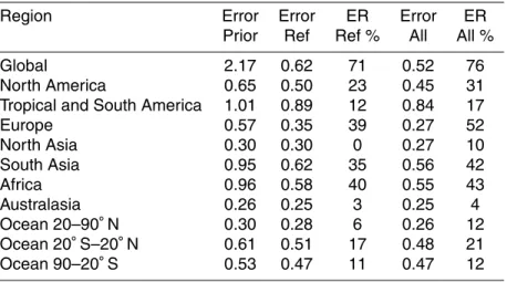
Figure 4 shows the annual mean error reduction per grid-cell calculated as one minus the ratio of the posterior to prior flux error, where the posterior error is found from the Monte Carlo ensemble of inversions, for the reference and full observation datasets. As expected, the distribution of error reduction is strongly dependent on the observational
10
network, with most of the reductions in the temperate northern latitudes. Despite the low error reduction at the grid-cell level in the tropics and Southern Hemisphere, mod-est error reductions are achieved by integrating the fluxes over regions. Table 5 shows the prior and posterior errors, and error reduction globally and for 8 land and 3 ocean regions. Using all observations, strong error reductions were found for Europe (52 %),
15
North America (31 %), South Asia (42 %) and Africa (43 %), while only moderate error reductions were found for South America (17 %), North Asia (10 %) and Australasia (4 %). The error reductions using only the reference sites were somewhat smaller, no-tably so for Europe, North America and South Asia, where during the inversion period new observation sites were established.
20
3.2 Mean spatial distribution
The mean spatial distribution (1999–2009) of the posterior fluxes did not differ signif-icantly between sensitivity tests, nor did the general distribution of the fluxes change remarkably throughout the 11 yr period. For this reason, only the mean flux from the control inversion, IAVA, is shown (Fig. 5). Tropical and subtropical regions exhibited
25
ACPD
13, 15697–15747, 2013N2O emissions 1999–2009 from a global atmospheric
inversion
R. L. Thompson et al.
Title Page
Abstract Introduction
Conclusions References
Tables Figures
◭ ◮
◭ ◮
Back Close
Full Screen / Esc
Printer-friendly Version Interactive Discussion
Discussion
P
a
per
|
Di
scussion
P
a
per
|
Discussion
P
a
per
|
Discussi
on
P
a
per
|
temperate North America (7 %), predominantly in the eastern states. This distribution is not unexpected and a similar pattern is also seen in the prior fluxes. All inversions, however, increased the flux relative to the prior in South and East Asia, and to a lesser extent in tropical Africa, North America, tropical South America and southern Europe (Fig. 6). In contrast, the inversions slightly reduced the mean flux in southern Africa,
5
southern South America, and in the Great Lakes region of North America.
Emissions from India and eastern China were found to be considerably more im-portant than predicted in the prior. This may be due to an underestimate of mineral nitrogen fertilizer application rates. These rates having been increasing rapidly in re-cent years but in the prior model the fertiliser rates from 2006 to 2009 were based on
10
2005 statistics, thus agricultural emissions in latter years may be underestimated in the prior. Another contributing factor may be an underestimate of reactive nitrogen deposi-tion rates; for instance, deposideposi-tion rates of NOy(an important denitrification substrate) are known to be systematically underestimated in India (Dentener et al., 2006). In gen-eral, both India and China have very high rates of NO3 (HNO3 and nitrate aerosol)
15
and NH+4 and NH3 deposition, which has likely also increased in recent years owing to increased nitrogen fertilizer usage and industrial activities (Dentener et al., 2006). Emissions from tropical western Africa were also found to be more important than pre-dicted in the prior, with flux levels comparable to those in eastern North America. This is somewhat surprising considering that the amount of mineral nitrogen fertilizer used in
20
tropical Africa is only a small fraction of that used in North America (Potter et al., 2010). Although we cannot rule out the possibility that the inversion over-estimates N2O emis-sions in tropical Africa, due to e.g. atmospheric transport errors, there are reasons why the prior flux may be an under-estimate. Statistics from this region are difficult to obtain, so there may be an under-reporting of fertilizer application rates. An additional factor
25
ACPD
13, 15697–15747, 2013N2O emissions 1999–2009 from a global atmospheric
inversion
R. L. Thompson et al.
Title Page
Abstract Introduction
Conclusions References
Tables Figures
◭ ◮
◭ ◮
Back Close
Full Screen / Esc
Printer-friendly Version Interactive Discussion
Discussion
P
a
per
|
Di
scussion
P
a
per
|
Discussion
P
a
per
|
Discussi
on
P
a
per
|
source of reactive nitrogen and may also be under-accounted for in O-CN (S. Zaehle, personal communication, 2012).
3.3 Temporal variability and trends
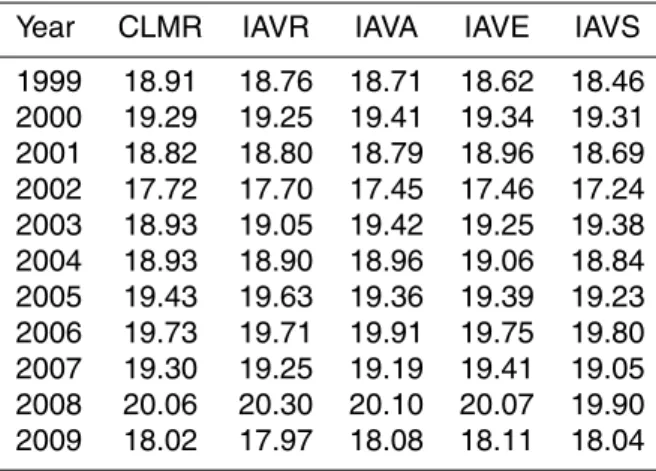
Over the 11 yr period, the global total N2O emission varied from 17.5 to 20.1 Tg a−1 N (for the inversion IAVA) and the year-to-year variation was significantly higher (0.77
5
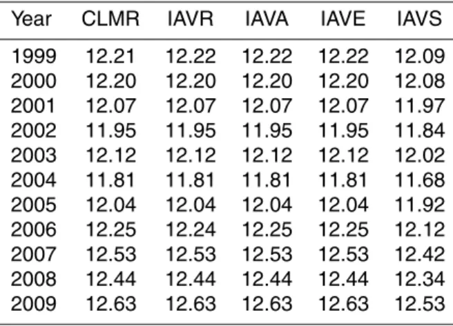
1 SD) than the variation between sensitivity tests for any given year (0.13 mean SD), and the uncertainty of 0.5 Tg a−1 N (Table 7). In contrast, there was little variability in the global total sink, which varied from 11.8 to 12.6 Tg a−1 N (Table 8). The years 2002 and 2009 stood out as having particularly low emissions (17.5 and 18.1 Tg a−1N, respectively) while in 2008 the emissions were the highest (20.1 Tg a−1N).
10
In addition to variations in the N2O source, the tropospheric mole fraction is influ-enced by variations in stratosphere to troposphere exchange (STE) as there is a strong gradient in N2O mole fraction across the tropopause, thus changes in the net air mass exchange between the stratosphere troposphere impact the tropospheric mole frac-tion (Nevison et al., 2011, 2007). Therefore, one important quesfrac-tion that arises is, how
15
sensitive are the inversion results to errors in the modelled STE? STE resulting in non-reversible transport of air masses to the troposphere is to a large extent driven by the Brewer–Dobson circulation (Holton et al., 1995). We have found that the seasonality of STE in the Northern Hemisphere is reasonably well resolved by LMDz and there is good agreement between modelled and observed seasonal cycles for CFC-12, which
20
has seasonality strongly dependent on STE. The agreement is poorer for the Southern Hemisphere, and here the error in the observation space was increased to account for this. Inter-annual variability in STE appears to be also reasonably well captured by LMDz, again based on comparisons of CFC-12 observed and modelled inter-annual variations (R=0.57 for the period 1996–2009) (Thompson et al., 2013).
25
ACPD
13, 15697–15747, 2013N2O emissions 1999–2009 from a global atmospheric
inversion
R. L. Thompson et al.
Title Page
Abstract Introduction
Conclusions References
Tables Figures
◭ ◮
◭ ◮
Back Close
Full Screen / Esc
Printer-friendly Version Interactive Discussion
Discussion
P
a
per
|
Di
scussion
P
a
per
|
Discussion
P
a
per
|
Discussi
on
P
a
per
|
prior and posterior annual flux anomalies integrated over each land region. Generally, the results for all sensitivity tests were in close agreement with one another. The fact that the test using a flux climatology as the prior (CLMR, orange) was close to the results using inter-annually varying prior fluxes provides confidence that the year-to-year variations are largely driven by the atmospheric observations. Furthermore, there
5
is good agreement between the results from the tests using the reference versus the full observation dataset indicating that a few sites are sufficient to capture flux inter-annual variability at (sub)-continental scales.
At the global scale, a weak positive trend in the N2O source was found (0.05 Tg a−2 N) but was not significant at the 95 % confidence level (pvalue of 0.5). The only
statis-10
tically significant trend was found in South Asia, where the source increased at a rate of 0.045 Tg a−2N (median of all sensitivity tests,pvalue of 0.006) between 1999 and 2009 (see Fig. 7). Although a similar trend (0.049 Tg a−2N) is seen in the prior fluxes, this signal is not only driven by the prior as the test CLMR also shows a similar trend.
4 Discussion
15
4.1 Emission trends in South Asia
The economies of South Asia, in particular those of China and India, have undergone rapid growth in the past decade. This has been seen in increased industrialisation and energy consumption. It has also led to a growing demand for food and thus an expansion and intensification of agriculture.
20
According to the Food and Agricultural Organization of the United Nations (FAO) statistics, nitrogen fertilizer consumption in China has increased on average by 0.66 Tg a−1 N between 2002 and 2010 (http://www.fao.org/corp/statistics/en/). During the same period, the total harvested area for all crops increased by 51 Mha leading to further increases in agricultural emissions. As a simple approximation, using a 1.25 %
25
ACPD
13, 15697–15747, 2013N2O emissions 1999–2009 from a global atmospheric
inversion
R. L. Thompson et al.
Title Page
Abstract Introduction
Conclusions References
Tables Figures
◭ ◮
◭ ◮
Back Close
Full Screen / Esc
Printer-friendly Version Interactive Discussion
Discussion
P
a
per
|
Di
scussion
P
a
per
|
Discussion
P
a
per
|
Discussi
on
P
a
per
|
et al., 1998), would lead to an increase of 0.008 Tg a−2 N. These calculations do not account for indirect N2O emissions associated with nitrogen leaching and atmospheric transport of reactive nitrogen, which lead to increased N2O emissions in areas remote from where the fertilizer was applied. A more complete estimate of the increase in agricultural emissions, which includes also indirect emissions, is given by the
EDGAR-5
4.2 inventory: on average 0.026 Tg a−2 N between 2000 and 2008. Increased energy consumption in China has also led to greater N2O emission, contributing 0.009 Tg a−2 N, and emissions from chemical production and solvent use contributing a further 0.002 Tg a−2 N (EDGAR-4.2). In total (i.e. across all sectors), EDGAR-4.2 estimates that Chinese N2O emissions have been increasing at an average rate of 0.042 Tg a−2
10
N (from 2000 to 2008).
In India, a similar trend in nitrogen fertilizer consumption is seen with an average increase of 0.68 Tg a−1N from 2002 to 2010 (FAO). In contrast to China, however, there has been negligible change in crop area. Furthermore, despite the strong increase in nitrogen fertilizer use, EDGAR-4.2 does not estimate a large change in agricultural
15
emissions of N2O, only 0.005 Tg a−2 N, nor in the total emissions, only 0.0075 Tg a−2 N, for 2000 to 2008. It is beyond the scope of this study to speculate on why there is an apparent discrepancy between the FAO statistics and the EDGAR-4.2 estimate for agricultural emissions. However, it is noteworthy that the average change in total emissions for China and India (approximately 0.05 Tg a−2 N) is in close agreement to
20
that found for South Asia by the inversions (0.045 Tg a−2N).
4.2 Inter-annual variability in fluxes
4.2.1 Tropical and subtropical land
The largest inter-annual variations in N2O emissions are seen in the tropical and sub-tropical land regions, i.e. Topical and South America, and Africa. In Fig. 7, periods
25
ACPD
13, 15697–15747, 2013N2O emissions 1999–2009 from a global atmospheric
inversion
R. L. Thompson et al.
Title Page
Abstract Introduction
Conclusions References
Tables Figures
◭ ◮
◭ ◮
Back Close
Full Screen / Esc
Printer-friendly Version Interactive Discussion
Discussion
P
a
per
|
Di
scussion
P
a
per
|
Discussion
P
a
per
|
Discussi
on
P
a
per
|
mid-2002 to 2003 and in 2007, with weak El Niño conditions between 2004 and 2006. The El Niño events of 2002 and 2007 coincide with low N2O flux anomalies, while, generally, La Niña conditions coincide with high N2O flux anomalies. (Unfortunately, there are insufficient accurate N2O measurements available prior to the late 1990s to resolve regional fluxes; hence, it is not possible to study the period of the strong El
5
Niño of 1997–1998.)
ENSO has a well-known climate impact in tropical and subtropical South America, Asia, Australia and South Africa (Trenberth et al., 1998, and references therein) and may be driving the changes in N2O land flux, as proposed by Thompson et al. (2013) and Ishjima et al. (2009). The strongest climate effects generally occur from
Decem-10
ber to February, and during an El Niño bring warm and dry conditions to the central and eastern parts of South America, South Africa and tropical and subtropical Asia. La Niña, on the other hand, is associated with cooler and wetter conditions in these regions. To investigate a possible link between climate and N2O flux, we analysed pre-cipitation, soil moisture, and temperature data from ECMWF ERA-interim (Dee et al.,
15
2011) at 80 km resolution. These meteorological parameters are known to strongly in-fluence the rates of denitrification and nitrification and to modulate N2O flux at the local scale (Davidson, 1993; Smith et al., 1998). The strong negative N2O flux anomaly in 2002 corresponds with negative precipitation and soil moisture anomalies over tropical and subtropical South America and Africa (see Fig. 10), in areas with significant mean
20
N2O flux (i.e. in areas with a mean soil N2O flux above 0.1 g m−2a−1N according to the prior flux estimate). Differences in N2O soil fluxes between e.g. the El Niño year 2002 and the near neutral year 2003 can be seen over Brazil and central Africa, where the flux is lower in 2002 (Fig. 9).
However, not all negative precipitation and soil moisture anomalies are associated
25
There-ACPD
13, 15697–15747, 2013N2O emissions 1999–2009 from a global atmospheric
inversion
R. L. Thompson et al.
Title Page
Abstract Introduction
Conclusions References
Tables Figures
◭ ◮
◭ ◮
Back Close
Full Screen / Esc
Printer-friendly Version Interactive Discussion
Discussion
P
a
per
|
Di
scussion
P
a
per
|
Discussion
P
a
per
|
Discussi
on
P
a
per
|
fore, the water limitation would need to be severe enough to make a significant change in WFPS. A severe drought could potentially also affect the availability of reactive nitro-gen in unfertilized regions by slowing the rate of mineralization of organic matter in soils (Borken and Matzner, 2009). An important link between soil moisture, mineralization rates and N2O flux in tropical soils on seasonal timescales has already been proposed
5
by Potter et al. (1996), and may also be important on inter-annual timescales. Fur-thermore, using a data-calibrated biogeochemical model, Werner et al. (2007) found significant inter-annual variability in the tropical rainforest soil N2O source, which was largely driven by changes in rainfall. For example, for African rainforests the N2O source was found to change by 0.21 Tg a−1N (50 %) from 1993 to 1994 (Werner et al., 2007),
10
a magnitude commensurate with changes found for Africa in the inversions. For com-parison, the change in N2O flux found by the inversions for tropical and subtropical South America, up to 0.6 Tg a−1N, represents about 20 % of the total mean flux of this region.
4.2.2 Temperate land
15
Inter-annual variations in temperate N2O soil fluxes, i.e. in North America, North Asia and Europe, are smaller than those found in the tropics. In North America, low N2O flux is found for 2005–2006 and coincides with negative precipitation and soil mois-ture anomalies in the ECMWF ERA-interim data (Dee et al., 2011) (see Fig. 10). In 2007, higher N2O fluxes are found and coincide with the return of precipitation rates
20
to average values. High fluxes are also seen in 1999, and coincide with a positive soil temperature anomaly and a weak positive anomaly in soil moisture. In Europe, low N2O flux is seen in 2005 and corresponds to a small negative anomaly in temperature, soil moisture and precipitation (see Fig. 10). Although significant negative anomalies in precipitation and soil moisture also occurred in 2003, no anomaly was seen in the
an-25
neg-ACPD
13, 15697–15747, 2013N2O emissions 1999–2009 from a global atmospheric
inversion
R. L. Thompson et al.
Title Page
Abstract Introduction
Conclusions References
Tables Figures
◭ ◮
◭ ◮
Back Close
Full Screen / Esc
Printer-friendly Version Interactive Discussion
Discussion
P
a
per
|
Di
scussion
P
a
per
|
Discussion
P
a
per
|
Discussi
on
P
a
per
|
ative flux anomaly of about 0.2 Tg a−1 N in the second half of 2003 and a positive anomaly of similar magnitude in the first half of the year, which cancel out in the annual total.
4.2.3 Ocean
Considerable inter-annual variability in N2O flux is also seen in the tropical (20◦N to
5
20◦S) and southern oceans (20 to 90◦S) (Fig. 8). In general, low N2O flux coincides with El Niño, in 2002 and 2007, and high N2O flux with La Niña, in 2000, 2006, and 2008. The inversion results are fairly consistent for all sensitivity tests. One notable exception is in the year 2006, where in the tropical ocean the inversion CLMR (using a climatological prior) stands out with a strong positive anomaly, which is not seen in the
10
other inversions for which the inter-annually varying prior was used. This discrepancy may be a result of too few degrees of freedom for the flux to depart from the prior N2O flux estimate, which is too low in the inter-annually varying fluxes.
ENSO has a strong influence on ocean upwelling and, thus, on air–sea gas ex-change. During El Niño, warm water in the Western Pacific migrates eastward and
15
reduces upwelling in the Eastern Pacific off the coast of South America, while during La Niña the process is reversed and there is an increase in upwelling (McPhaden et al., 2006). Changes in upwelling affect air–sea N2O fluxes through physical and biological processes. Physically, by changing the supply of N2O-rich water from below the eu-photic zone to the surface and thereby the partial pressure of N2O in the surface water,
20
and biologically, by changing the supply of nutrients to the surface layer and thus pri-mary production and the production of N2O within the surface layer (Nevison et al., 2007). These processes are parameterized in the biogeochemistry model, PISCES, used for the prior ocean N2O flux in the inversion (Dutreuil et al., 2009). PISCES was coupled to a climate model and is thus sensitive to ENSO driven changes. However,
25
ACPD
13, 15697–15747, 2013N2O emissions 1999–2009 from a global atmospheric
inversion
R. L. Thompson et al.
Title Page
Abstract Introduction
Conclusions References
Tables Figures
◭ ◮
◭ ◮
Back Close
Full Screen / Esc
Printer-friendly Version Interactive Discussion
Discussion
P
a
per
|
Di
scussion
P
a
per
|
Discussion
P
a
per
|
Discussi
on
P
a
per
|
driven changes in ocean N2O flux and verifies the magnitude of these changes, which are on the order of 0.4 Tg a−1N globally.
5 Summary and conclusions
We present estimates of N2O fluxes from 1999 to 2009 based on the inversion of atmo-spheric transport and observations of atmoatmo-spheric N2O mole fractions. To determine
5
the sensitivity of the inversion results to the coverage of the observations, the prior fluxes used, the strength of the stratospheric sink, and the assigned observation error, 5 different inversion tests were carried-out. All 5 inversions produced consistent results within the posterior error margin, which indicates a fair representation of the prior errors in the inversion system. Over the 11 yr period, the global total N2O source varied from
10
17.5 to 20.1 Tg a−1N (control inversion, IAVA) with a SD of 0.77 Tg a−1N. The year-to-year variability in the global source was significantly larger than the variability between inversions in any given year (0.13 Tg a−1N mean SD). Tropical and subtropical land re-gions were found to have the highest N2O emissions; in particular, South Asia (20 % of global total), Tropical and South America (13 %) and Africa (19 %), while the temperate
15
regions of Europe (6 %) and North America (7 %) were less important. A global trend in the N2O source of 0.05 Tg a−2 N was detected but was not significant at the 95 % confidence level. The only significant trend in N2O emissions was in the region of South Asia (0.045 Tg a−2N) and is consistent with inventory estimates from EDGAR-4.2. This trend appears to be primarily driven by increasing agricultural emissions (about 60 %
20
of the trend) and, secondarily, by increased energy consumption (about 20 %). Inter-annual variability in the global N2O source was largely driven by variability in tropical and subtropical soil fluxes, in particular, in Tropical and South America (0.3 Tg a−1 N 1 SD) and to a lesser extent in Africa (0.3 Tg a−1 N 1 SD). Significant variability was also found in N2O fluxes in the tropical and southern oceans (0.15 and 0.2 Tg a−1N 1
25
ACPD
13, 15697–15747, 2013N2O emissions 1999–2009 from a global atmospheric
inversion
R. L. Thompson et al.
Title Page
Abstract Introduction
Conclusions References
Tables Figures
◭ ◮
◭ ◮
Back Close
Full Screen / Esc
Printer-friendly Version Interactive Discussion
Discussion
P
a
per
|
Di
scussion
P
a
per
|
Discussion
P
a
per
|
Discussi
on
P
a
per
|
ENSO, where El Niño conditions are associated with lower N2O fluxes and vice-versa for La Niña. The mechanism for the ENSO–N2O relationship is most likely through cli-mate changes in tropical and subtropical South America and Africa affecting soil N2O fluxes and through changes in upwelling in the eastern Pacific affecting the ocean N2O flux. ENSO-driven changes in the land and ocean fluxes are in the same direction and,
5
thus, reinforce the change in the tropospheric N2O mole fraction. These results show that the tropospheric N2O mole fraction is sensitive to climate-driven changes in soil and ocean N2O fluxes. Furthermore, the climate-driven global N2O source variability (∼1 Tg a−1 N) is substantially larger than the current rate of increase in the source (∼0.1 Tg a−2 N), indicating that climate is a significant factor in modulating the annual
10
global N2O-budget.
Acknowledgements. We are very grateful for the input and feedback from Sönke Zaehle, Lau-rent Bopp and William Lahoz. We thank Guido van der Werf for use of the GFED data and the EDGAR team for the use of their inventory data. We also acknowledge the support of the LSCE computing services. This work was jointly financed by the European Commission under the EU
15
Seventh Research Framework Programme (grant agreement No. 283576. MACC-II) and by the Norwegian Research Council (contract No. 193774, SOGG-EA).
References
Bergamaschi, P., Krol, M., Meirink, J. F., Dentener, F., Segers, A., van Aardenne, J., Monni, S., Vermeulen, A. T., Schmidt, M., Ramonet, M., Yver, C., Meinhardt, F., Nisbet, E. G.,
20
Fisher, R. E., O’Doherty, S., and Dlugokencky, E. J.: Inverse modeling of European CH4
emissions 2001–2006, J. Geophys. Res., 115, D22309, doi:10.1029/2010jd014180, 2010. Borken, W. and Matzner, E.: Reappraisal of drying and wetting effects on C and N mineralization
and fluxes in soils, Glob. Change Biol., 15, 808–824, 2009.
Bousquet, P., Peylin, P., Ciais, P., Le Quéré, C., Friedlingstein, P., and Tans, P. P.: Regional
25
ACPD
13, 15697–15747, 2013N2O emissions 1999–2009 from a global atmospheric
inversion
R. L. Thompson et al.
Title Page
Abstract Introduction
Conclusions References
Tables Figures
◭ ◮
◭ ◮
Back Close
Full Screen / Esc
Printer-friendly Version Interactive Discussion
Discussion
P
a
per
|
Di
scussion
P
a
per
|
Discussion
P
a
per
|
Discussi
on
P
a
per
|
Bousquet, P., Ciais, P., Miller, J. B., Dlugokencky, E. J., Hauglustaine, D. A., Prigent, C., Van der Werf, G. R., Peylin, P., Brunke, E. G., Carouge, C., Langenfelds, R. L., Lathière, J., Papa, F., Ramonet, M., Schmidt, M., Steele, L. P., Tyler, S. C., and White, J.: Contribution of anthropogenic and natural sources to atmospheric methane variability, Nature, 443, 439– 443, 2006.
5
Bouwman, A. F.: Environmental science: nitrogen oxides and tropical agriculture, Nature, 392, 866–867, 1998.
Bouwman, A. F., Boumans, L. J. M., and Batjes, N. H.: Modeling global annual N2O and NO emissions from fertilized fields, Global Biogeochem. Cy., 16, 1080, doi:10.1029/2001GB001812, 2002.
10
Chevallier, F., Fisher, M., Peylin, P., Serrar, S., Bousquet, P., Bréon, F.-M., Chédin, A., and Ciais, P.: Inferring CO2sources and sinks from satellite observations: method and application
to TOVS data, J. Geophys. Res., 110, D24309, doi:10.1029/2005JD006390, 2005.
Chevallier, F., Bréon, F.-M., and Rayner, P. J.: Contribution of the orbiting carbon observatory to the estimation of CO2sources and sinks: theoretical study in a variational data assimilation
15
framework, J. Geophys. Res., 112, D09307, doi:10.1029/2006JD007375, 2007.
Corazza, M., Bergamaschi, P., Vermeulen, A. T., Aalto, T., Haszpra, L., Meinhardt, F., O’Doherty, S., Thompson, R., Moncrieff, J., Popa, E., Steinbacher, M., Jordan, A., Dlugo-kencky, E., Brühl, C., Krol, M., and Dentener, F.: Inverse modelling of European N2O
emis-sions: assimilating observations from different networks, Atmos. Chem. Phys., 11, 2381–
20
2398, doi:10.5194/acp-11-2381-2011, 2011.
Crutzen, P. J., Mosier, A. R., Smith, K. A., and Winiwarter, W.: N2O release from agro-biofuel
production negates global warming reduction by replacing fossil fuels, Atmos. Chem. Phys., 8, 389–395, doi:10.5194/acp-8-389-2008, 2008.
Davidson, E. A.: Soil water content and the ratio of nitrous to nitric oxide emitted from soil,
25
in: Biogeochemistry of Global Change: Radiatively Active Trace Gases, edited by: Orem-land, R. S., Chapman and Hall, London, 369–386, 1993.
Dee, D. P., Uppala, S. M., Simmons, A. J., Berrisford, P., Poli, P., Kobayashi, S., Andrae, U., Balmaseda, M. A., Balsamo, G., Bauer, P., Bechtold, P., Beljaars, A. C. M., van de Berg, L., Bidlot, J., Bormann, N., Delsol, C., Dragani, R., Fuentes, M., Geer, A. J., Haimberger, L.,
30