www.hydrol-earth-syst-sci.net/18/819/2014/ doi:10.5194/hess-18-819-2014
© Author(s) 2014. CC Attribution 3.0 License.
Hydrology and
Earth System
Sciences
Winter stream temperature in the rain-on-snow zone of the Pacific
Northwest: influences of hillslope runoff and transient snow cover
J. A. Leach1and R. D. Moore1,2
1Department of Geography, University of British Columbia, 1984 West Mall, Vancouver, British Columbia, Canada 2Department of Forest Resources Management, University of British Columbia, 1984 West Mall,
Vancouver, British Columbia, Canada
Correspondence to:J. A. Leach ([email protected])
Received: 1 October 2013 – Published in Hydrol. Earth Syst. Sci. Discuss.: 31 October 2013 Revised: 20 January 2014 – Accepted: 23 January 2014 – Published: 27 February 2014
Abstract. Stream temperature dynamics during winter are less well studied than summer thermal regimes, but the win-ter season thermal regime can be critical for fish growth and development in coastal catchments. The winter ther-mal regimes of Pacific Northwest headwater streams, which provide vital winter habitat for salmonids and their food sources, may be particularly sensitive to changes in cli-mate because they can remain ice-free throughout the year and are often located in rain-on-snow zones. This study ex-amined winter stream temperature patterns and controls in small headwater catchments within the rain-on-snow zone at the Malcolm Knapp Research Forest, near Vancouver, British Columbia, Canada. Two hypotheses were addressed by this study: (1) winter stream temperatures are primarily controlled by advective fluxes associated with runoff pro-cesses and (2) stream temperatures should be depressed dur-ing rain-on-snow events, compared to rain-on-bare-ground events, due to the cooling effect of rain passing through the snowpack prior to infiltrating the soil or being delivered to the stream as saturation-excess overland flow. A reach-scale energy budget analysis of two winter seasons revealed that the advective energy input associated with hillslope runoff overwhelms vertical energy exchanges (net radiation, sensi-ble and latent heat fluxes, bed heat conduction, and stream friction) and hyporheic energy fluxes during rain and rain-on-snow events. Historical stream temperature data and mod-elled snowpack dynamics were used to explore the influence of transient snow cover on stream temperature over 13 win-ters. When snow was not present, daily stream temperature during winter rain events tended to increase with increasing air temperature. However, when snow was present, stream
temperature was capped at about 5◦C, regardless of air tem-perature. The stream energy budget modelling and historical analysis support both of our hypotheses. A key implication is that climatic warming may generate higher winter stream temperatures in the rain-on-snow zone due to both increased rain temperature and reduced cooling effect of snow cover.
1 Introduction
response to future land cover and climatic changes (Webb et al., 2008; Arismendi et al., 2012).
Most stream temperature research has been concerned with summer temperatures, particularly in response to ri-parian forest disturbance such as harvesting or wildfire (e.g. Johnson and Jones, 2000; Bartholow, 2005; Gaffield et al., 2005; Gomi et al., 2006; Gravelle and Link, 2007; Leach and Moore, 2010; Janisch et al., 2012; Imholt et al., 2013). This summer-focused research consistently identifies energy exchanges occurring at the stream surface (primarily net radiation) as a key control on temperature variability on diurnal to seasonal scales and the response to changes in ri-parian canopy conditions. In some reaches, however, surface-water–groundwater interactions can significantly moderate temperature variability (e.g. Johnson, 2004; Moore et al., 2005; Leach and Moore, 2011; MacDonald et al., 2014).
In contrast to the depth and breadth of research on sum-mer stream temperature, few studies have examined winter stream temperature processes despite its recognized impor-tance for aquatic ecosystems (Beschta et al., 1987; Holtby, 1988; Ebersole et al., 2006; Brown et al., 2011; Shuter et al., 2012). Salmonids are poikilothermic, so decreases in stream temperature correspond with declines in metabolic processes and the ability of fish to swim, feed, and avoid predators (Brown et al., 2011). Therefore, predation by homeother-mic predators during winter is believed to be high, partic-ularly when surface ice cover is non-existent or incomplete (Huusko et al., 2007; Watz et al., 2013). In many temperate regions, particularly the coastal portions of the Pacific North-west of North America (PNW), headwater catchments expe-rience moderate air temperatures and transient snow cover. As a result, headwater streams in these regions typically re-main unfrozen during most of the winter, and their thermal regimes may be particularly sensitive to changes in winter air temperature and precipitation. Under these conditions, even a relatively small (e.g. 1–2◦C) but persistent change to stream temperature could have a significant effect on fish bioener-getics and on rates of growth and development of inverte-brates that dominate salmonid food sources (Brown et al., 2011; Arismendi et al., 2013).
Winter in coastal portions of the PNW region is charac-terized by frequent cloud cover and precipitation. Therefore, solar radiation should be a less important control on stream temperature than in summer, especially considering the low solar elevation angles. Although we are unaware of any pub-lished wintertime stream energy budgets in the coastal por-tion of the PNW, studies from sites outside this region have found that magnitudes of energy exchanges occurring at the stream surface are smaller during winter than during summer periods (Webb and Zhang, 1997, 1999; Hannah et al., 2008; Leach and Moore, 2010). An important characteristic of the coastal portion of the PNW is that, at low to medium eleva-tions, frequent rain and rain-on-snow events maintain high flows, which could result in substantial lateral advection of thermal energy via hillslope runoff.
This study addressed two hypotheses: (1) winter stream temperatures in headwater catchments of the rain and rain-on-snow zones of the PNW region are primarily controlled by advective fluxes associated with runoff processes dur-ing storm events, and (2) stream temperatures should be de-pressed during snow events, compared to rain-on-bare-ground events, due to the cooling effect of rain pass-ing through the snowpack prior to infiltratpass-ing the soil or being delivered to the stream as saturation-excess overland flow. The hypotheses were addressed using field data col-lected at headwater catchments within the rain-on-snow zone at the Malcolm Knapp Research Forest, near Vancouver, British Columbia, Canada. A diagnostic energy budget anal-ysis was conducted using data collected during the winters of 2011/2012 and 2012/2013 from a heavily instrumented catchment and supplemented with 13 yr of historical stream temperature data (1997–2002, 2007–2008, and 2010–2013) and modelled snowpack dynamics for an adjacent catchment to explore winter thermal regimes and the role of transient snow cover. The methodology and results of the energy bud-get study are presented in Sect. 3, followed by the method-ology and results of the historical study in Sect. 4. The two complementary studies are discussed together in Sect. 5.
2 Study area
Research was conducted at the University of British Columbia’s Malcolm Knapp Research Forest, located at 49◦16′N and 122◦34′W, about 60 km east of Vancouver
Fig. 1.Map of Griffith Creek and East Creek study catchments.
flows downslope in a saturated layer above the contact be-tween the soil and underlying till or bedrock. Most stormflow occurs in the autumn–winter wet season and many streams dry up during the summer.
Griffith Creek was the focus of the energy budget study. At the location of a hydrometric weir, it drains an area of 11 ha, ranging from 365 to 572 m a.s.l. Temperature data for East Creek were used in the historical analysis. At the loca-tion of the temperature logger, East Creek’s catchment has an area of 44 ha and ranges in elevation from 280 to 447 m a.s.l. East Creek’s catchment was logged in the 1920s and is cur-rently covered by mature forest stands about 80 yr old, with crown closures of 75–95 %. Griffith Creek’s catchment had similar forest cover until autumn of 2004, when the lower section of the catchment was logged under a partial retention approach, resulting in 50 % of the basal area being removed and a 14 % reduction in canopy closure (Guenther et al., 2012). Currently, the lower section’s vegetation cover is com-posed of sparse mature trees and a shrub understory about 1–3 m in height. The shrub understory experiences consider-able dieback during the winter months. The upper portion of Griffith Creek’s catchment is covered by mature forest simi-lar to that in East Creek’s catchment. For the energy budget analysis the stream was divided into two reaches, which are
referred to herein as the “harvest” and “forest” reaches. The harvest reach was bounded by Q1 and Q2 and was 220 m in length with a slope of 0.09 mm−1 and classified as a step–
pool morphology; the forest reach was bounded by Q2 and Q3 and was 340 m in length with a slope of 0.16 mm−1and classified as step–pool and cascade (Fig. 1). Wetted channel widths varied with discharge but generally averaged 1 m or less for both reaches. Griffith and East Creek catchments are characterized by high topographic relief, which provide sub-stantial terrain shading. Channels are not heavily incised and shading from channel banks is minimal. East Creek supports a population of coastal cutthroat trout (Oncorhynchus clarki clarki) (De Groot et al., 2007).
3 Energy budget study at Griffith Creek
3.1 Data collection
Field data were collected at Griffith Creek from Octo-ber 2011 to May 2013. Field measurements were aimed at quantifying the energy and water balance components for use within a diagnostic energy budget for two stream reaches. Details of these measurements are provided below.
3.1.1 Precipitation and snowpack
At a meteorological station located at a recent clearcut, hereinafter referred to as the open site (Fig. 1), a tipping bucket rain gauge was used to measure liquid precipita-tion, a bulk precipitation gauge measured rain and snow-fall, and a snow lysimeter measured snowmelt and rainfall. The bulk precipitation gauge consisted of a 1.2 m length of PVC pipe (20.32 cm diameter) that was sealed at the bottom and equipped with a pressure transducer. The pipe contained antifreeze to melt snow and was topped with a thin layer of mineral oil to minimize evaporation. The tipping bucket and bulk precipitation gauges were logged by Campbell Sci-entific CR10x loggers and data were stored every 10 min. The snow lysimeter (4 m2area and 0.0625 mm per tip) was constructed following the design by Smith (2011) and was logged with an Em5b data logger (Decagon Devices, Pull-man, Washington). Total drainage from the lysimeter (rain-fall plus snowmelt) was stored every 1 h.
Two additional snow lysimeters with the same specifi-cations as the open-site lysimeter were installed at Griffith Creek, one in the harvested area and one in the unharvested area. Both sites also had tipping bucket rain gauges installed below the forest canopy, which were used to confirm occur-rence of rainfall.
sampler. A minimum of five density measurements were made at each site. Snowpack water equivalent was computed as the product of mean depth and mean density, divided by the density of liquid water.
Time-lapse cameras installed at the open site and the Grif-fith Creek harvest and forest sites captured images daily at 09:00, 12:00 and 15:00 PST (Pacific Standard Time). Im-ages were used to map snow extent and cover and, in con-junction with meteorological data, help identify occurrence of rain-on-snow events (Floyd and Weiler, 2008).
3.1.2 Streamflow and channel geometry
Streamflow was monitored at the Griffith Creek catchment outlet (Q1) as well as at two additional locations along the stream reach (Q2 and Q3) (Fig. 1). The drainage areas for Q1, Q2 and Q3 are 10.8, 6.6, and 0.8 ha, respectively. Man-ual streamflow measurements were made using the constant-rate salt dilution injection method (Moore, 2004). Stream-flow measurements were accurate to±5 %, based on repli-cated gauging. The Q1 station had a v-notch weir and pres-sure transducer, whereas Q2 and Q3 were outfitted with still-ing wells and pressure transducers. Ratstill-ing curves were de-veloped for each location in order to estimate continuous streamflow records.
Average wetted width and depth of the stream were deter-mined from measurements made at 25 locations distributed along Griffith Creek (11 and 14 in the harvest and forest reaches, respectively). Sixteen sets of 25 width and depth surveys were made over a range of stream discharges. Mean width and depth for the lower harvested and upper forested reaches were regressed against discharge in order to fit em-pirical power–law relations for predicting width and depth for the entire study period. Mean widths ranged between 0.49 and 0.97 m with a relative standard error of ±21 % for the harvest reach, and 0.28 and 0.62 m (±19 %) for the forest reach. Mean depths ranged between 0.10 and 0.27 m (±26 %) for the harvest reach, and 0.08 and 0.21 m (±37 %) for the forest reach.
3.1.3 Stream temperature
Eight submersible temperature loggers (Tidbit v2 Temp, On-set Computer Corporation, accurate to±0.2◦C) were dis-tributed along Griffith Creek. Three of the locations used in this study correspond to streamflow gauging sites Q1, Q2, and Q3. Temperature loggers were installed at sites with suf-ficient water depth so that loggers were not exposed during low flows. The loggers were shielded with white PVC pipe with drilled holes to facilitate water exchange. Sensors were logged at 15 min intervals and averaged every 1 h. Sensors were calibrated at 0 and 20◦C (in an ice bath and at room temperature, respectively), before and after field deployment. Vertical and lateral manual spot measurements were made using a WTW 340i handheld conductivity and temperature
meter (accurate to±0.1◦C) at each logger site during site
visits to ensure that the logger was placed in a location with full vertical and lateral mixing. Manual spot measurements were also used to check logger records for drift throughout the study.
3.1.4 Above-stream microclimate
Two automated weather stations were installed at sites within 2 m of the Griffith Creek channel to characterize the above-stream microclimate in the forested and harvested reaches. The weather stations monitored air temperature with a HMP45C-L probe (accurate to±0.3◦C), relative humidity with a HMP45C-L probe (accurate to±3 % for the 0–90 % relative humidity range and±5 % for the 90–100 % relative humidity range), incoming solar radiation with a CMP3 Kipp and Zonen pyranometer, wind speed with a Met One 3-cup anemometer (starting threshold of 0.45 m s−1) at
approxi-mately 1.5 m above the ground surface, and rainfall at the ground surface with a tipping bucket rain gauge (0.254 mm per tip). All sensors were scanned every 10 s and averaged (or summed for the rain gauges) every 10 min by Campbell Scientific CR10x data loggers.
Above-stream net radiation was measured using a roving Kipp and Zonen net radiometer to test predictions from a net radiation model (details provided below). The net radiome-ter was set up at 14 locations (six and eight locations in the forest and harvest reaches, respectively) along Griffith Creek during the study period in order to sample spatial variabil-ity in net radiation due to variable riparian vegetation struc-ture. At each location, the net radiometer was positioned ap-proximately 30–40 cm above the stream surface. The sensor was scanned every second and readings were averaged every 10 min using a Campbell Scientific CR10x logger.
3.1.5 Subsurface water levels and temperature
Shallow groundwater levels were monitored at 50 wells that were installed by hand augering to the soil–till interface (mean depth was approximately 0.6 m). Wells were made from PVC pipe (35 mm inside diameter) with holes drilled along the lower half and screened with permeable garden fab-ric to prevent soil movement into the well. The wells were located within 5–10 m of the stream in order to character-ize throughflow inputs to the channel. Wells were located to sample a range of hillslope sizes and shapes determined from different topographic indices, including upslope con-tributing area and topographic wetness index. Forty wells were outfitted with Odyssey capacitance water level loggers (Dataflow Systems Pty Ltd, Christchurch, New Zealand) to provide 15 min-interval water level records. The remaining wells were monitored manually once a week during the win-ter period. The groundwawin-ter well network was surveyed us-ing a total station.
Soil temperatures were recorded within 1 m of 40 of the groundwater wells. At four sites, soil temperatures were recorded by thermocouples at three depths (0.05, 0.25 and 0.5 m), which were connected to Campbell Scientific CR10x data loggers. Thirty-six of the groundwater well sites were fitted with submersible temperature loggers installed at the soil–till interface using a hand auger and backfilled after in-stallation. Four of these sites had an additional soil temper-ature logger installed at a second depth above the soil–till interface. In addition, soil temperatures were recorded at two depths (0.05 and 0.15 m) at each of the snow lysimeter sites located within the Griffith Creek catchment. All soil temper-ature sensors logged data at 15 min intervals with the excep-tion of the snow lysimeter sites, where soil temperatures were logged at 60 min intervals. Temperature loggers were deter-mined to be below or above the water table at each time step based on the known depth of the temperature logger and the corresponding well water level.
Piezometers were installed in the centre of the streambed at 25 locations at approximately even spacing along the study reach. At four step–pool sequences, piezometers were in-stalled upstream of the step and downstream in the pool. Piezometers were constructed from 6 mm-internal-diameter plexiglass tubing with holes drilled in the bottom 5 cm, and were installed to depths of 10–30 cm below the streambed. Vertical hydraulic gradients were computed as the differ-ence in water level between the inside and outside of the piezometer, divided by the depth of the mid-point of the per-forated section (Scordo and Moore, 2009). Positive hydraulic gradients indicate upwelling flow. Water levels inside and outside the piezometers were measured with an electronic beeper and accurate to±5 mm (Guenther, 2007). Piezome-ters were also used to measure saturated hydraulic conductiv-ity of the bed sediments using a falling-head slug test (Freeze and Cherry, 1979). Hydraulic conductivity (Ksat) was
com-puted based on an equation derived by Hvorslev (1951) and
modified by Baxter et al. (2003) for closed-bottom perforated piezometers.
At each of the 25 piezometer locations, thermocouples were installed within the streambed. Twenty-two locations had three thermocouples installed at various depths and three locations had two thermocouples, due to the shallow depth of bed sediment. Thermocouple depths varied by location and ranged between 0.02 and 0.3 m depending on the ease of in-stallation, which was determined by differences in streambed composition and depth to bedrock. Vertical hydraulic gradi-ents, bed temperatures, and hydraulic conductivity were mea-sured once a month during winter site visits. Based on previ-ous studies reported in the literature and at sites within Mal-colm Knapp Research Forest (Moore et al., 2005; Guenther, 2007), we anticipated that bed heat conduction and hyporheic energy fluxes would be secondary terms in the energy bud-get and therefore devoted more resources to estimating the other fluxes. We performed spot measurements to provide a basis for confirming that these fluxes were indeed secondary terms.
3.2 Analysis
A reach-scale energy budget analysis was used to assess the relative importance of the various energy fluxes controlling winter stream temperatures at Griffith Creek. In the follow-ing sections we outline the methods used to measure and es-timate the various energy exchanges acting on the stream, followed by a description of the reach-scale energy budget equations. Note that the term “surface energy fluxes” is de-fined as net radiation, and sensible and latent heat fluxes oc-curring at the stream surface; “vertical energy fluxes” is de-fined as surface fluxes, bed heat conduction, and stream fric-tion; and “lateral energy fluxes” is defined as advective fluxes from surface runoff and throughflow.
3.2.1 Net radiation
at the two pyranometer sites. Using the optimized thresh-old, mean hourly net radiation was modelled and evaluated against measured net radiation at each of the 14 roving net ra-diometer locations using the associated hemispherical image. For the energy budget, hourly reach-scale mean net radiation (Q∗in W m−2) was modelled for both the forested and
har-vested reach using hemispherical images from the respective reaches.
3.2.2 Latent and sensible heat fluxes
The latent heat flux (Qein W m−2) was computed using an
empirical wind function fitted to evaporimeter data collected at Griffith Creek for both pre- and post-harvest conditions (Guenther et al., 2012):
Qe =627.8 [0.0424·U·(ea−ew)], (1)
whereU is wind speed (m s−1); ea andew are the vapour
pressures of air and water, respectively (kPa); and 627.8 ac-counts for the unit conversion from mm h−1to W m−2. Satu-ration vapour pressure (esatin kPa) was calculated as a
func-tion of air or water temperature,Ta or Tw (◦C), using the
following relation:
esat(T )=0.611·exp
a T
T +b
(2) whereT is in◦C, and the coefficientsaandbare given by (a,
b) = (17.27, 237.26) forT >0◦C and (a,b) = (21.87, 265.5)
forT≤0◦C. The vapour pressure at the water surface,ew,
was assumed to equalesat(Tw), while the actual vapour
pres-sure of the air (ea) was calculated as ea =
RH
100
esat(Ta) , (3)
where RH is the relative humidity measured at the nearest stream microclimate station.
The sensible heat flux (Qh) was estimated as
Qh =β ·Qe (4)
whereβis the Bowen ratio, calculated as
β =0.66·(P /1000)·(Tw−Ta) / (ew−ea), (5)
where P is ambient air pressure, which was assigned the value for a standard atmosphere for the site elevation (97 kPa).
3.2.3 Bed heat conduction and hyporheic energy exchange
Spot estimates of bed heat conduction,Qc, were calculated
as
Qc =Kc·(Tb−Tw) /0.05, (6)
whereKc is the thermal conductivity of the streambed
ma-terial (W m−1K−1), andT
b andTw are bed temperature at
depth of 0.05 m and stream temperature, respectively. The thermal conductivity was assumed to equal 2.6 W m−1K−1 based on estimates of Lapham (1989) using a porosity of 0.30, which is typical for gravels (Freeze and Cherry, 1979).
The heat flux associated with hyporheic exchange,Qhyp,
for the combined forest and harvest reaches was estimated as
Qhyp=ρ cpFhyp Thyp−Tw/W, (7)
whereρis the density of water (1000 kg m−3);c
pis the
spe-cific heat of water (4180 J kg−1K−1);F
hypis hyporheic
ex-change rate per unit length of channel (m3s−1m−1); T hyp
andTw are the temperatures of upwelling hyporheic water
and stream water, respectively; andW is the mean stream width (m). The mean of streambed temperatures from up-welling sites was used forThyp.Qhypwas not calculated
sep-arately for the forest and harvest reaches because of the lim-ited number of piezometer and streambed temperature sites available to computeFhypandThyp.
A reach-scale estimate ofFhyp was computed by
assum-ing that all water infiltratassum-ing the bed within the reach follows subsurface flow paths that discharge within the same reach. It was further assumed that the fraction of the total bed area that experiences downwelling is equal to the fraction of the piezometers with downwelling flow. Following from these assumptions,Fhypwas computed as
Fhyp = ndw/npiezo·A·qz/L, (8)
wherendw andnpiezo are the number of piezometers
indi-cating downwelling flow and the total number of piezome-ters, respectively;Ais the area (m2) of the streambed;qzis
the vertical flux of water infiltrating the streambed (m s−1); andL is the reach length (m). The area of the streambed was computed as the product of reach length and mean sur-face width, which was computed from the fitted relation with discharge.
Infiltration rates were estimated based on Darcy’s Law:
qz =Ksat· |1h/1z| (9)
whereKsatis the saturated hydraulic conductivity of the bed
(m s−1), determined from slug tests, and1h/1zis the mean
vertical hydraulic gradient from piezometers that registered downwelling flow.
3.2.4 Stream friction
Heat generated by fluid friction as water flows downstream,
Qf(W m−2), was computed as
whereg is the gravitational acceleration (9.81 m s−2);Qis
the reach-average discharge (m3s−1), which is assumed to
be equal to the mean of the upstream and downstream dis-charges;Sis the slope of the reach (mm−1) extracted from a 5 m resolution digital elevation model of the catchment; and
Wis the average wetted width of the stream reach (m).
3.2.5 Lateral heat fluxes calculated as residual of stream energy budget
Energy budget analyses were conducted for the 2011/2012 and 2012/2013 winter periods (1 October to 1 May) for the harvest reach and the forest reach. The longitudinal heat transfer (Ji) was calculated at 10 min time steps at each
gaug-ing site as
Ji =ρ·cp·Qi ·Ti, (11)
whereQi is the discharge (m3s−1), andTi is the stream
tem-perature, at gauging sitei.
The difference betweenJi+1 andJi is equal to the sum
of the net heat input to the reach and change in heat stor-age within the reach. This energy budget formulation does not require knowledge of travel times. The storage term was found to be negligible and is not included in the calculation of lateral advective heat flux, described below. The energy ex-changes at the stream surface (net radiation, sensible, and la-tent heat) and stream friction were estimated using the mod-elling approach described above and were subtracted from the net heat input to the reach. The residual was attributed to the lateral advective heat input (Jadv):
Jadv =Ji+1−Ji −L·W ·(Q∗+Qh+Qe+Qf) , (12)
whereLis the length of the stream reach (m);W is the av-erage wetted width of the stream reach (m); andQ∗,Qh, Qe, andQfare the fluxes of net radiation, sensible heat,
la-tent heat, and heat inputs due to stream friction (W m−2), respectively.
3.2.6 Effective lateral inflow temperature
The effective lateral inflow temperature (Tadv) was calculated
as
Tadv =Jadv/(Qi+1−Qi)·ρ ·cp. (13)
The calculated value ofTadv was compared to the 40
mea-surements of near-stream soil temperature. To explore how
Tadv responded to different hydroclimatic event types, daily
means ofTadvwere calculated and each day during the study
was classified as (1) rain on ground, (2) rain on snow, (3) no precipitation and bare ground, or (4) no precipitation and snow cover.
3.2.7 Error analysis
A standard approach for error analysis (Bevington and Robinson, 2003) was applied to the stream energy budget
−5
0
5
10
15
Air temper
ature (
°
C)
●
●
● ●
● ●
●
● 2011/12 2012/13
Oct Nov Dec Jan Feb Mar Apr
0
200
400
Precipitation (mm/month)
● ●
● ●
● ●
●
Fig. 2.Boxplots of monthly (October to April) mean air tempera-ture and monthly total precipitation recorded at the MKRF head-quarters station from 1962 to 2010. Red circles and blue squares represent conditions during the two winter periods (2011/2012 and 2012/2013, respectively) during which the detailed field study at Griffith Creek was conducted.
calculations in order to assess uncertainty. The propa-gated probable error was determined using the following values: Q∗±22 W m−2, Qe±25 %, Qh±25 %, Q±5 %, Tw±0.2◦C,L±10 %,S±20 %,W±21 % (harvest reach)
and ±19 % (forest reach). The values for Q∗, Q, W, and
Tw were determined from uncertainty assessments of field
measurements, whereas the remaining errors were deemed to be reasonable estimates that erred in the direction of overestimation.
3.3 Results
3.3.1 Overview of study period
Figure 2 places the 2011/2012 and 2012/2013 field seasons within a broader climatic context using long-term (1962 to 2013) climate data from the MKRF headquarters station. Monthly mean air temperatures for October to April for the two field seasons were generally within the middle 50 % of historic values. There was more variability in precipitation patterns, as October through December of 2011/2012 was dry relative to historic conditions, whereas precipitation dur-ing the 2012/2013 season was generally similar to or well above the long-term median.
Discharge (L/s)
Q1 (weir) Q2 (mid) Q3 (top)
0.01
1
100
0
5
10
15
Stream temp (
°
C) Q1 (weir)
Q2 (mid) Q3 (top)
−5
5
15
Air temp (
°
C)
0
5
10
15
W
ater input (mm/h)
Snow cover
Nov Jan Mar May
2011/12
Oct Dec Feb Apr
2012/13
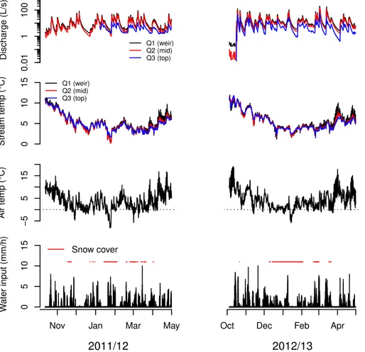
Fig. 3.Hydroclimatic overview for the 2011/2012 and 2012/2013 winter periods (October to May). Water input refers to rainfall and snowmelt measured by the snow lysimeter located at the open site.
discharge was generally more responsive to rain events in 2012/2013, particularly for the Q3 site. This difference in discharge response between the two years was similar for other headwater catchments in the research forest (data not shown).
Mean hourly stream temperatures varied between 1 and 12◦C during the study period (Fig. 3). Mean hourly lon-gitudinal stream temperature differences between Q1, Q2, and Q3 were often less than 0.5◦C. However, in April, tem-peratures at Q1 tended to be about 1◦C greater than at Q2 and Q3 during the day. Maximum diurnal range in hourly temperatures at Q1 were 3.2 and 3.4◦C for 2011/2012 and
2012/2013, respectively. Mean diurnal range in hourly tem-peratures was 0.9◦C for both winters. Stream temperature
did not have a consistently positive or negative relation with discharge, but seemed to vary with discharge depending on the antecedent air and stream temperatures. Mean hourly air temperatures fell below 0◦C for only short periods (less than one week) during winter.
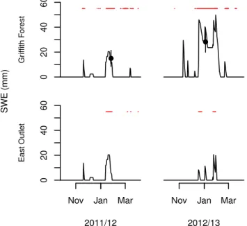
Total water input (rainfall plus snowmelt) measured at the open-site lysimeter for the study periods (1 October to 1 May) was 1736 mm for 2011/2012 and 1950 mm for
2012/2013. The 2011/2012 winter had 52 days of snow cover in the forested area and 63 days in the harvested area, spread over a number of events, whereas the 2012/2013 winter had 71 days of snow cover in both forested and harvested areas, mostly due to a snowpack that persisted from 14 December to 25 January.
3.3.2 Energy balance
Hourly modelled net radiation was compared to measured net radiation at the 14 net radiometer locations during the study period. The root mean square error and mean bias error ranged between 17 and 22, and−18 and−6 W m−2,
respec-tively, across the 14 sites. These errors are similar to those found in previous efforts to model above-stream net radiation from hemispherical photographs (Leach and Moore, 2010; Bulliner and Hubbart, 2013).
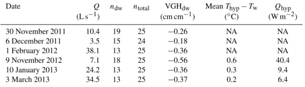
Table 1.Summary of discharge (Q), number of piezometers indicating downwelling flow (ndw), total number of piezometers measured (ntotal), reach-average vertical hydraulic gradient forndw(VGHdw), mean temperature difference betweenThyp−Twfor upwelling sites, and estimated reach averageQhyp. NoteThypwas not measured for the first three dates.
Date Q ndw ntotal VGHdw MeanThyp−Tw Qhyp
(L s−1) (cm cm−1) (◦C) (W m−2)
30 November 2011 10.4 19 25 −0.26 NA NA
6 December 2011 3.5 15 24 −0.18 NA NA
1 February 2012 38.1 13 25 −0.36 NA NA
9 November 2012 7.1 18 25 −0.56 0.6 40.4
10 January 2013 24.2 13 25 −0.36 0.3 9.4
3 March 2013 34.5 13 25 −0.37 0.2 6.4
weaker than our winter measurements. Table 1 shows the number of piezometers with downwelling flow, total number of piezometers sampled, vertical hydraulic gradients calcu-lated for piezometers with downwelling flow, reach-average differences betweenThypandTwfor the upwelling locations,
andQhyp estimates for six dates when all piezometer sites
were sampled. For flows below about 10 L s−1, up to al-most 80 % of the piezometers registered downwelling flow, with the fraction dropping to just over 50 % at higher flows. Temperature differences betweenThypandTwwere less than
0.7◦C and estimates of the reach-average heat transfer asso-ciated with hyporheic exchange were less than 50 W m−2. Both the fraction of piezometers registering downwelling flow and the difference in hyporheic and stream tempera-tures decreased with increasing discharge, suggesting that the energy transfer associated with hyporheic exchange also clines with increasing discharge. Although we did not de-termine separate values of Qhyp for the forest and harvest
reaches due to the small number of samples, the limited data suggest that there was not a substantial difference between the reaches in terms of Thyp and percentage of
piezome-ters with downwelling flow. For bed heat conduction calcu-lations, temperature gradients between the stream and bed were small during all spot measurements and across all loca-tions. Temperature differences between the stream and bed at depths of 15 cm were less than 0.8◦C and often less than 0.2◦C. Estimates of bed heat conduction were less than
15 W m−2.
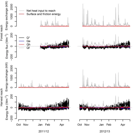
Figure 4 shows estimated hourly surface energy fluxes and the heat inputs due to stream friction for the harvest and forest reaches for 2011/2012 and 2012/2013. Net radi-ation was the dominant surface energy flux. Hourly net ra-diation ranged between−70 and 150 W m−2for the harvest reach and−60 and 120 W m−2for the forest reach, whereas the sensible and latent heat exchanges at both reaches never exceeded ±30 W m−2. During the months of November to February for both 2011/2012 and 2012/2013, net radiation was mostly an energy loss from the stream. Starting in late February, net radiation was an energy source to the stream during day and a sink during night. Heat generated by
frictional dissipation of potential energy averaged between 15 and 30 W m−2 over the study periods and ranged be-tween 0.2 and 219 W m−2for the harvest reach and 4.8 and 218 W m−2for the forest reach. Heat inputs due to friction were greatest during high flows.
Figure 4 summarizes the reach-scale energy budget anal-ysis for the 2011/2012 and 2012/2013 winter periods at the harvest and forest reaches. Except during low-flow periods, when lateral inputs of water became relatively small, the ver-tical energy exchanges were only a small fraction of the to-tal heat input into either the harvest or forest reaches even accounting for uncertainty in the flux estimates. Figure 5 il-lustrates that, for discharges above approximately 25 L s−1,
surface energy fluxes account for less than 2 % of the heat input to the reach. For discharges below 25 L s−1, surface
en-ergy fluxes can account for a considerable proportion of the net reach heat input, both as a heat source and sink, as in-dicated by positive or negative ratios, respectively, in Fig. 5. Most of the highly negative ratios correspond with periods of large relative errors in the heat budget calculations, par-ticularly due to the small changes in discharges along the reach. Surface fluxes were, on average, 4.6 and 4.5 % of the net heat input to the forest reach during the 2011/2012 and 2012/2013 winter periods, respectively, and slightly greater at 9.3 and 5.9 % during 2011/2012 and 2012/2013, respec-tively, for the harvest reach. However, during some low-flow periods, when advective inputs and heat generated by fric-tion were minimal, the surface fluxes accounted for nearly the entire change in longitudinal heat flux along the reaches. The pattern of net heat input into the reaches followed that of discharge, which highlights lateral advection as a dominant heat input to the stream reach. The generally higher magni-tude of net heat inputs for 2012/2013 vs. 2011/2012 reflects the higher magnitude of streamflow that year. Relative mag-nitudes of the surface energy inputs between the forest and harvest reaches were similar between the two years.
3.3.3 Effective lateral inflow temperature