www.solid-earth.net/1/5/2010/
© Author(s) 2010. This work is distributed under the Creative Commons Attribution 3.0 License.
Solid Earth
Earth’s surface heat flux
J. H. Davies1and D. R. Davies2
1School of Earth and Ocean Sciences, Cardiff University, Main Building, Park Place, Cardiff, CF103YE, Wales, UK 2Department of Earth Science & Engineering, Imperial College London, South Kensington Campus, London, SW72AZ, UK
Received: 5 November 2009 – Published in Solid Earth Discuss.: 24 November 2009 Revised: 8 February 2010 – Accepted: 10 February 2010 – Published: 22 February 2010
Abstract. We present a revised estimate of Earth’s surface heat flux that is based upon a heat flow data-set with 38 347 measurements, which is 55% more than used in previous estimates. Our methodology, like others, accounts for hy-drothermal circulation in young oceanic crust by utilising a half-space cooling approximation. For the rest of Earth’s surface, we estimate the average heat flow for different ge-ologic domains as defined by global digital geology maps; and then produce the global estimate by multiplying it by the total global area of that geologic domain. The averag-ing is done on a polygon set which results from an intersec-tion of a 1 degree equal area grid with the original geology polygons; this minimises the adverse influence of clustering. These operations and estimates are derived accurately using methodologies from Geographical Information Science. We consider the virtually un-sampled Antarctica separately and also make a small correction for hot-spots in young oceanic lithosphere. A range of analyses is presented. These, com-bined with statistical estimates of the error, provide a mea-sure of robustness. Our final preferred estimate is 47±2 TW, which is greater than previous estimates.
1 Introduction
Heat flow measurements at Earth’s surface contain integrated information regarding the thermal conductivity, heat produc-tivity and mantle heat flux below the measurement point. By studying Earth’s surface heat flux on a global scale, we are presenting ourselves with a window to the processes at work within Earth’s interior, gaining direct information about the internal processes that characterize Earth’s ‘heat engine’. The magnitude of the heat loss is significant compared to
Correspondence to:J. H. Davies
other solid Earth geophysical processes. Consequently, the study and interpretation of surface heat flow patterns has be-come a fundamental enterprise in global geophysics (Lee and Uyeda, 1965; Williams and Von Herzen, 1974; Pollack et al., 1993).
The global surface heat flux provides constraints on Earth’s present day heat budget and thermal evolution mod-els. Such constraints have been used to propose exciting new hypotheses on mantle dynamics, such as layered con-vection with a deep mantle interface (Kellogg et al., 1999), and that D” is the final remnant of a primordial magma ocean (Labrosse et al., 2007). One class of thermal evolu-tion models are the so-called parameterised convecevolu-tion mod-els (Sharpe and Peltier, 1978). While such models have been examined for several years, they have recently been re-energised, with work in fields including: (i) alternative ther-mal models (Nimmo et al., 2004; Korenaga, 2003); (ii) re-fined estimates of mantle radioactive heating (Lyubetskaya and Korenaga, 2007a); (iii) estimates of core-mantle heat flow, following from observations of double crossing of the perovskite/post-perovskite phase transition (Hernlund et al., 2005); and (iv) advances in models of the geodynamo (Chris-tensen and Tilgner, 2004; Buffett, 2002). Earth’s global sur-face heat flux plays a fundamental role in all of the above.
In this study, we use Geographical Information Science (GIS) techniques, coupled with recently developed high-resolution, digital geology maps, to provide a revised es-timate of Earth’s surface heat flux. We employ a signifi-cantly (55%) larger data-set (38 347 data points) than pre-vious work. While we focus on our preferred value, we also present a range of possible values based upon a variety of as-sumptions. This, combined with careful estimation of errors, provides a rigorous error estimate.
The structure of the paper is as follows. A brief intro-duction to the work of PHJ93 is first presented, along with some background to our related methods. The heat flow and geology data-sets used are then described. This is fol-lowed by a description of our methodology, including the corrections, which are guided by JLM07. The actual re-sults and, importantly, the errors, are then presented and dis-cussed. We conclude by discussing our preferred estimate of 47 TW, (rounded from 46.7 TW given that our error esti-mate is±2 TW) which is greater than recent estimates. We note, however, that this value overlaps with JLM07, when considering the associated errors (±2 TW). Such error esti-mates are of great importance; our total error of around 2 TW is less than JLM07 (3 TW) but double the 1 TW of PHJ93.
2 Methods
Heat flow observations are sparse and non-uniformly dis-tributed across the globe. Pollack et al. (1993) (PHJ93) show that even on a 5×5 degree grid, observations from their data-set cover only 62% of Earth’s surface. Therefore, to obtain a global estimate of surface heat flow, PHJ93 derived empiri-cal estimators from the observations by referencing the heat flow measurements to geological units. The underlying as-sumption is of a correlation between heat flow and surface geology. In this way, it is possible to produce estimates of surface heat flow for regions of the globe with no observa-tions (this could also be thought of as an area weighted av-erage based upon geological category). PHJ93 did this by first attributing every 1×1 degree grid cell to a specific ge-ology. The heat flow data in each cell was then averaged and resulting cell values were used to estimate an average heat flow for each geology. An estimate was produced glob-ally for each geological unit by evaluating its area in terms of 1×1 degree grid-cells and multiplying by the estimated mean heat flux derived for that geology. The total heat flux was evaluated by summing the contribution of each geologi-cal unit. Finally, estimates were made for hydrothermal cir-culation in young oceanic crust, using the model of Stein and Stein (1992) (hereafter abbreviated to SS).
There has been a major revolution in the handling of spa-tial data in the intervening years, with the growth of GIS. GIS allows geological units to be defined by high-resolution irregular polygons in digital maps. The highest resolution geology data-set (a combination of two data-sets) utilised in
this study has over 93 000 polygons. GIS allows us to evalu-ate the areas of these geology units exactly (to mapping accu-racy) and to also match heat flow measurements with specific local geology. PHJ93 had to estimate the area of geological units by dividing Earth’s surface into 1×1 degree equal lon-gitude, equal latitude cells. They then hand-selected the pre-dominant geology of each cell and summed the number of cells. Such a methodology could potentially generate errors in the estimates of geological unit areas. In addition, in cells with greater than one geological unit, this could lead to heat flow measurements being associated with the incorrect geol-ogy. Further advantages of GIS methods include the ability to:
1. Easily match heat flow measurements with individual geology polygons;
2. Undertake accurate re-calculations with different grids and for different geology data-sets;
3. Use equal area grids (rather than equal longitude grids); 4. Make robust error estimates, weighted by area.
2.1 Heat flow data-set
(a)
(b)
(c)
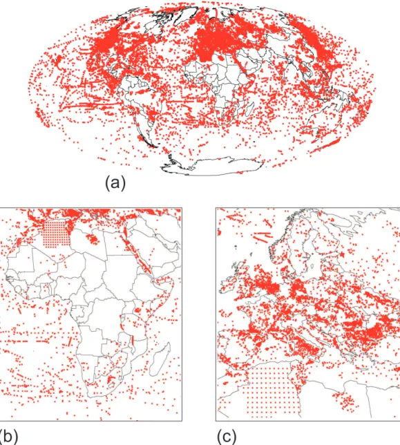
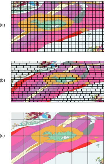
Fig. 1. (a)Global distribution of heat flow measurements, showing the inhomogeneous distribution of data-points. This suggests that
extrapolations to develop a global heat flux estimate might benefit from utilising any global indicator that might be correlated with heat flow. In this study, we use geology for this purpose, following the work of Pollack et al. (1993).(b)Focussed on the African continent – note the sparsity of data points.(c)Focussed on Europe, where good coverage is apparent, particularly in areas such as the Central North Sea, Black Sea and Tyrrhenian Sea, where interest in surface heat flow has been extensive due to exploration and tectonism.
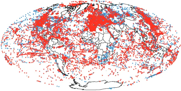
Figure 1 illustrates the global distribution of the data-set, clearly showing the inhomogeneous spread of measure-ments. Figure 2 includes a breakdown of the new data-set into new points, those points included in PHJ93, and those modified from PHJ93, while histograms of the heat flow measurements are given in Fig. 3. We stress, like PHJ93, that while the histograms of the ocean and continental heat flow measurements look similar, this is misleading. The oceanic region is dominated by sites with sediment cover and these are known to be biased systematically downwards by hydrothermal circulation (Davis and Elderfield, 2004).
Fig. 2.As in Fig. 1a, but broken down into those points included in PHJ93 (blue) and additional points (red).
Frequency
Heat Flow (mW m )-2
(a)
0 2000 4000 6000
0 50 100 150 200 250 300 350 400 Global Oceanic Continental
Frequency
Heat Flow (mW m )-2
(b)
0 2000 4000 6000
0 50 100 150 200 250 300 350 400 D D 10 Extra Modified Exact
Fig. 3. (a)Histogram of heat flow measurements (global, oceanic
and continental) grouped by value of measurement, in bins of 10.
(b)A breakdown of the data-set used in this study (DD10), into those points replicated in PHJ93 (exact), those points modified from PHJ93 (modified) and additional points (extra).
2.2 Geology data-sets
We utilise two geology data-sets:
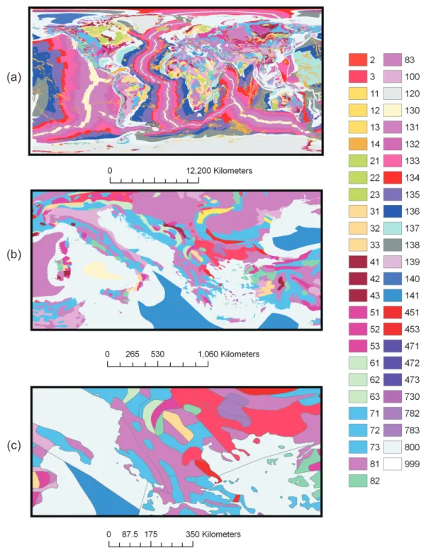
1. A global data-set, CCGM/CGMW (Commission for the Geological Map of the World, 2000), abbreviated to CCGM (the French initials for the data-set – Commis-sion de la Carte G´eologique du Monde). It ascribes ev-ery point on Earth’s surface to a geological unit (see Fig. 4).
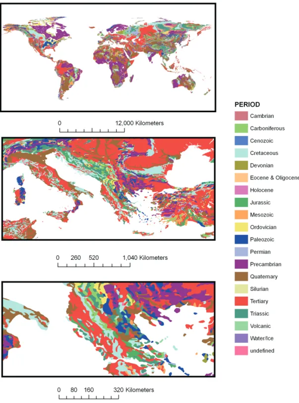
2. A data-set of continental geology (Hearn et al., 2003), abbreviated to GG – for Global GIS. It includes virtu-ally all land above sea-level, excluding Antarctica and Greenland (see Fig. 5).
(a)
(b)
(c)
Fig. 4.Geology as given by Commission for the Geological Map of the World – CCGM (2000):(a)Global view;(b)focussed on South-East
Europe;(c)focussed at higher-resolution in South-East Europe.
assigned to one of three classes (either igneous, sedimentary or other (endogeneous – plutonic or metamorphic)). For GG, the continental rocks are divided by geologic period, with no further division according to rock type. The GG clas-sification therefore has more periods than PHJ93 but does not subdivide them according to rock type. Figure 6 shows
Fig. 5.Geology (GG) as given by Hearn et al. (2003):(a)Global view(b)focussed on South-East Europe,(c)focussed at high-resolution in South-East Europe.
While we have already commented on the fact that there is a strong variation in the density of heat flow observations we should also note that there is a strong spatial variation in the detail of geological classification provided by the digital
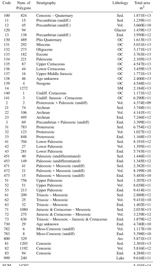
Table 1. Breakdown of the Geology in the Commission for the Geological Map of the World (2000), which we abbreviate to CCGM in the text. Sed – sedimentary rocks (or undifferentiated facies); end – endogenous rocks (plutonic and/or metamorphic); arc – continental and island arc margins; vol – extrusive volcanic rocks; SM – seamount, oceanic plateau, anomalous oceanic crust; OC – oceanic crust; undiff – undifferentiated.
Code Num. of Stratigraphy Lithology Total area
Polygons m2
100 824 Cenozoic – Quaternary Sed. 1.871E+13
11 15 Precambrian (undiff.) Sed. 1.239E+11
12 45 Precambrian (undiff.) Vol. 3.660E+10
120 94 Glacier 1.439E+13
13 138 Precambrian (undiff.) End. 3.950E+12
130 489 Plio-Quaternary OC 1.613E+13
131 292 Miocene OC 5.031E+13
132 273 Oligocene OC 3.171E+13
133 182 Eocene OC 3.763E+13
134 221 Paleocene OC 2.105E+13
135 87 Upper Cretaceous OC 4.547E+13
136 44 Lower Cretaceous OC 3.459E+13
137 16 Upper-Middle Jurassic OC 1.771E+13
138 46 Age unknown OC 2.406E+13
139 4 Neogene OC 4.548E+11
14 1272 SM 2.184E+13
140 1 Undiff. Cretaceous OC 1.171E+12
141 3 Undiff. Jurassic - Cretaceous OC 6.290E+11
2 2 Proterozoic + Paleozoic (undiff) Vol. 4.374E+09
21 74 Archean Sed. 3.748E+11
22 106 Archean Vol. 4.141E+11
23 495 Archean End. 7.246E+12
3 69 Precambrian + Paleozoic (undiff) End. 3.399E+11
31 783 Proterozoic Sed. 6.754E+12
32 123 Proterozoic Vol. 1.027E+12
33 848 Proterozoic End. 1.168E+13
41 704 Lower Paleozoic Sed. 8.191E+12
42 27 Lower Paleozoic Vol. 1.395E+11
43 281 Lower Paleozoic End. 5.743E+11
451 40 Paleozoic (undifferentiated) Sed. 1.446E+11
453 149 Paleozoic (undifferentiated) End. 1.345E+12
471 41 Paleozoic + Mesozoic (undiff) Sed. 2.382E+11
472 21 Paleozoic + Mesozoic (undiff) Vol. 8.199E+10
473 15 Paleozoic + Mesozoic (undiff) End. 5.485E+10
51 756 Upper Paleozoic Sed. 1.207E+13
52 51 Upper Paleozoic Vol. 8.658E+11
53 213 Upper Paleozoic End. 9.414E+11
61 209 Triassic – Mesozoic Sed. 2.880E+12
62 25 Triassic – Mesozoic Vol. 9.431E+10
63 32 Triassic – Mesozoic End. 1.402E+11
71 1080 Jurassic & Cretaceous – Mesozoic Sed. 2.033E+13
72 275 Jurassic & Cretaceous – Mesozoic Vol. 3.239E+12
73 636 Triassic – Mesozoic – Jurassic & Cretaceous End. 1.879E+12
730 29 Age unknown End. 4.740E+10
782 6 Meso-Cenozoic (undiff) Vol. 1.117E+10
783 8 Meso-Cenozoic (undiff) End. 5.398E+10
800 329 Arc 5.871E+13
81 1203 Cenozoic Sed. 2.301E+13
82 1192 Cenozoic Vol. 5.816E+12
83 94 Cenozoic End. 4.284E+11
999 240 Lake 9.616E+11
Table 2.Breakdown of the geology in Hearn et al. (2003), Global GIS (abbreviated as GG in the text).
Period Number of Total Area Number of heat polygons (m2) flow measurements
Cambrian 2541 3.378E+12 160
Carboniferous 3591 3.413E+12 349
Cenozoic 486 2.431E+11 4
Cretaceous 8492 1.287E+13 1661
Devonian 3268 3.617E+12 353
Eocene & Oligocene 39 2.122E+11 2
Holocene 485 1.706E+11 26
Jurassic 5376 5.394E+12 579
Mesozoic 5200 3.536E+12 245
Ordovician 1825 2.391E+12 200
Paleozoic 7145 4.820E+12 681
Permian 2463 3.421E+12 390
Precambrian 11895 2.871E+13 1563
Quaternary 12063 2.968E+13 2927
Silurian 1558 1.723E+12 92
Tertiary 18026 2.304E+13 6147
Triassic 3463 4.537E+12 482
Volcanic 442 7.290E+10 5
Water/Ice 395 5.721E+11 87
Undefined 3211 1.050E+12 380
Total 91964 1.328E+14 16333
2.3 Grids
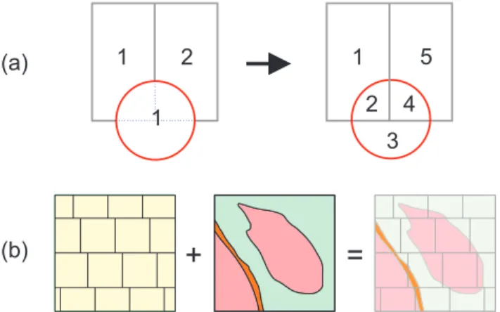
PHJ93 used a 1×1 degree equal longitude grid (64 800 grid cells) (see Fig. 6a for an example) in their analysis. We have undertaken our preferred analysis using a 1×1 degree equal area grid, with 41 252 cells in total. These cells are 1×1 degree at the equator, but at pole-ward latitudes the cell longitudes increase to approximate equal area. In this way, each cell has the same and equal weight (see Fig. 6b for an illustration of this grid in the North Atlantic). The difference between an equal area and equal longitude grid is greatest at high latitudes. Since there are limited heat flow observations at high latitudes, we expect that the improvement of using an equal area grid might be limited in this study. Amongst our range of investigations we also used a 5×5 degree equal longitude grid (see Fig. 6c).
2.4 Analysis
To better illustrate the impact of various aspects of the methodology, we have undertaken a series of alternative anal-yses, giving us a handle on the level of uncertainty in our estimate. We shall next describe, in detail, the methodology used in our preferred analysis, since this is the most com-plex. This will allow us to more easily describe the other analyses, without having to repeat the complete description of each stage:
(a)
(b)
(c)
Fig. 6.Presentation of CCGM Geology, focussed on the North
At-lantic, together with 3 different grids:(a)1 degree equal longitude grid;(b)1 degree equal area grid; and(c)5 degree equal longitude grid.
1. We plotted up all CCGM and GG geology. We then erased the GG geology from the CCGM geology (i.e. the areas covered by the GG data-set are removed from the CCGM data-set, such that recombining the re-sulting data-set with the GG data-set leads to complete global coverage, with no overlap).
1 1
1
3 4
5 2
2
+
=
(a)
(b)
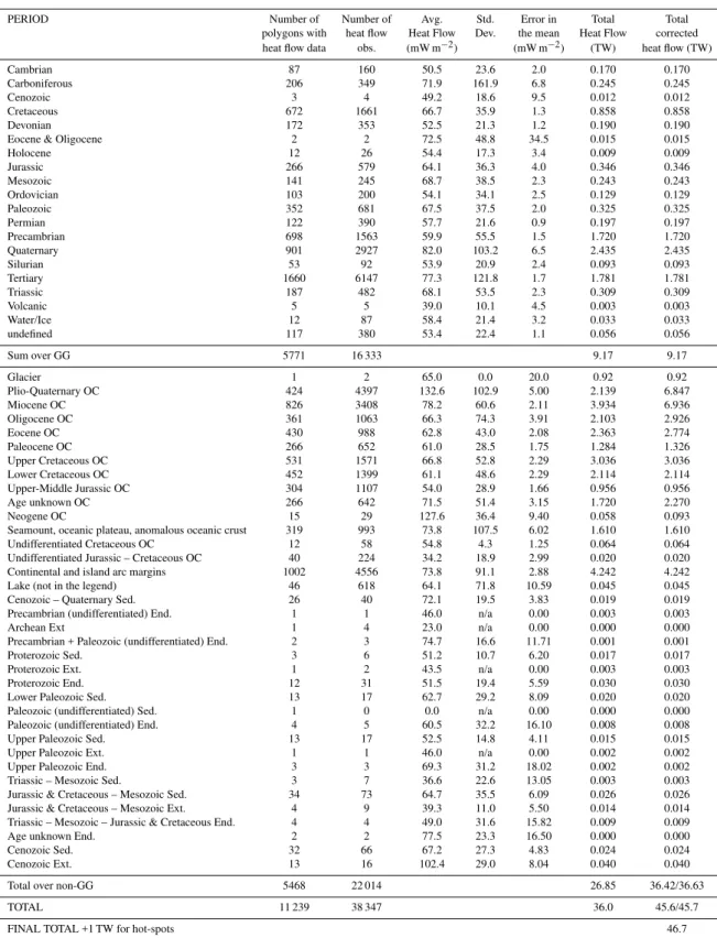
Fig. 7.The process of unioning:(a)We illustrate the union process
with two rectangles in the first layer and one circle in the second layer. Following union the resultant layer, in this case, has 5 poly-gons, none of which are circular or rectangular. We note that the number of polygon features in the output layer is greater than the number of polygons in either input layer. Any polygon on either input layer can be made up from a number of polygons in the out-put layer. The resultant layer has the attributes ofbothinput layer polygons in its attribute table;(b)a schematic of how the process would look for the grid and geology polygons.
clustering that exists in the heat flow data-set; by using the union methodology, large geologic regions do not get dominated by measurements from one heavily stud-ied site. It should be noted that both PHJ93 and Jaupart et al. (2007) (JLM07) utilise 1 degree equal longitude grids to minimise the effects of clustering.
3. The resulting polygons were spatially joined to the heat flow data. In the spatial join, the attributes of the geol-ogy polygon containing the heat flow point is added to the table of attributes of the heat flow points (i.e. each heat flow point has its geology associated with it – see Fig. 8).
4. The mean heat flow for each geology polygon (unioned with the grid as described above) was calculated, pro-ducing a new output (summary) table (see Fig. 9). The geology label of each polygon and the average heat flow was stored in the summary table.
5. The mean heat flow value was calculated for each geol-ogy class using the summary table of the previous step. This, again, was a straightforward arithmetic mean of all polygons that had non-zero heat flow polygons for each specific geology.
6. The global area of each geological unit was calculated. 7. The final estimate of the global average heat flow was
evaluated by assuming that the average heat flow found for each geology could be assigned to all similar geol-ogy (i.e. for each geological category, its average heat
flow was multiplied by its global area to find its contri-bution to the global heat flux).
We follow JLM07 and PHJ93 and make an estimate for hy-drothermal circulation, assuming that the heat flow in young oceanic crust is best described by a half-space model. Un-like PHJ93 who used the parameters of SS, we have used the value suggested by JLM07, but have also repeated the analy-sis using the parameters of Parsons and Sclater (1977) (here-after abbreviated to PS) and SS, to examine the differences and uncertainties arising from these models. Thus, for all geology younger than 66.5 Ma (66.4 Ma for 1983 timescale) we have replaced the heat flow obtained from the raw data with a value obtained from the equation:
q=C/√t (1)
where q is surface heat flux (mW m−2), C is a constant
(mW m−2Myr0.5), and t is the age of the oceanic
litho-sphere in millions of years. The value ofC preferred by JLM07 is 490±20 mW m−2Myr0.5; while the values of SS and PS are 510 and 430 mW m−2Myr0.5, respectively. The error of JLM07 is small, partly because they use the con-straint that at infinite age the half-space model should pre-dict zero heat flux. While that is certainly correct, it might be over optimistic to believe that a half-space model with a single constant is the correct model, at least as fit through all the data selected over such a wide range. We note that JLM07 ignore data at old age, since the half-space model is known not to fit that data well (that miss-fit led to the devel-opment of plate models), and at very young age, since the high variability reduce their usefulness in constraining the parameters. As a result we take a slightly more conserva-tive estimate of the error inCand assume errors 50% greater (i.e.±30 mW m−2Myr0.5at 2 standard deviations).
Table 3 shows the results for the 56 individual geology units (the 20 units on the continents from GG, and the 36 units from CCGM that represent the rest of the globe not included in the GG data-set) for this case. As described above, the final result is produced by multiplying the average heat flow calculated for each geology by the global area for that geology. Notice that some geological units have no (or very few) heat flow measurements. However, these make up only a very small proportion of the total area (1.5%, for less than 50 readings (excluding the Glacier category, which is discussed below and makes up∼3% of area)). For cases of geology with insufficient readings for the area to be included, we have shared the area among similar regions.
A
B C
A
B C
Point
Polygon Polygon Attributes Point Attributes
Point Attributes Polygon Attributes A A 1 B B 1 C C 2 1 1 2 2 Spatial Join
Fig. 8. Schematic illustrating the spatial join between a layer with three points and a second layer of two polygons. The process adds the
attributes of the appropriate polygon that contains the point of interest. This is how we assign a geology to each heat flow measurement.
Summarise on Geology
Original Table Summarised Table
Geology
Geology MeanValue Frequency Further Attribute A Further Attribute B Further Attribute C Heat Flow Value A A 3 1 1 B C 56.2 59.57 78.7 33.7 67.6 54.9 33.7 78.7 B C A A ... ... ... ... ... ... ... ... ... ... ... ... ... ... ...
Fig. 9.Schematic illustrating the process of producing a summary
table. A target field is selected, in this case geology. The process “summarises” selected fields in defined manners e.g. mean, sum, standard deviation, that correspond to each unique entry in the se-lection field. In the example illustrated, the mean heat flow has been summarised for each geology category. The summary table will also contain the number of rows (heat flow measurements) contributing to each summary value.
is not a perfect predictor of the heat flow); and (iii) the fact that large areas of Africa, Antarctica and Greenland are un-sampled. Errors in the area could arise due to poor definition of geological boundaries in the digital geology maps. We do not estimate such errors here. However, we find that our es-timate of continent (ocean) area is slightly greater (less) than JLM07, but as JLM07 point out, since the total area is fixed, these differences have only a small effect. The issue of the inadequate extrapolation and the poor coverage is more sig-nificant as a source of error and is later discussed in detail.
We have decided to include a value for the Glacier cate-gory in our preferred analysis. The Glacier catecate-gory of the CCGM geology covers 3% of Earth’s surface area, primarily across Greenland and Antarctica. Depending upon the ex-act methodology used, we get between 2 and 5 final readings (grid, geology), and a mean heat flow value of between 105 and 120 mW m−2, which is probably far too high a value. An estimate of 65 mW m−2was recently made for the heat flux in Antarctica, from estimates of the depth to the Curie tem-perature, based upon magnetic field measurements (Maule et al., 2005). The work of Shapiro and Ritzwoller (2004) also refers to the problem of estimating the heat flow of
Antarc-tica, in this case using seismic measurements as a proxy. They suggest that the heat flow in West Antarctica is almost a factor of three higher, and more variable (more like the small number of actual heat flow observations in our data-set), than in East Antarctica, where the heat flow has an estimated “lo-cal mean” of 57 mW m−2. Since East Antarctica has a larger area than West Antarctica (by a factor of∼3), the work of Shapiro and Ritzwoller (2004) would also argue for an over-all value for Antarctica closer to 65 mW m−2rather than the
∼105–120 mW m−2given by the raw measurements. While
this is similar to current predictions of the average heat flow through continents, it must be viewed as an uncertain esti-mate. However, our preference is to use this estimate and (105–65) mW m−2as the two standard deviation estimate of the error (105 mW m−2 being the minimum direct estimate from the data).
In Table 4 we list the heat flow and geology data-sets, the grids, and the methods used for the various alternative anal-yses undertaken. Each case is next described in detail:
1. While we have not repeated the work of PHJ93, in our first analysis, we used their heat flow data-set (taken from Gosnold and Panda, 2002), a 5×5 degree equal longitude grid and their methodology of selecting ogy for the whole of a cell, based on the majority geol-ogy of that cell. However, we used the CCGM geolgeol-ogy data-set.
2. As in Case 1, but using the new heat flow data-set (DD10).
3. As in Case 2, but a spatial join was undertaken between the heat flow data and the underlying geological poly-gons.
4. As in Case 3, but, in addition, we undertook a union between the geology and a 1 degree equal area grid. 5. As in Case 3, but with the combination of GG and
CCGM geology data-sets.
Table 3. Detailed breakdown of the preferred analysis for Earth’s surface heat flux. The raw data yields heat flow estimates of 105– 120 mW m−2for the Glacier category (113.5 mW m−2in the preferred analysis); the value of 65 mW m−2listed here comes from Maule et al. (2005), with the error estimate based on the difference between 105 and 65 mW m−2. The raw total, with no young ocean crust heat flow estimate, is 36.0 TW. The total over the GG geology is 9.2 TW. The total over the non-GG geology, including the young ocean estimate is 36.4 TW, while 36.6 TW is the value after allowance is made for ignoring geology classes with<50 readings. Therefore, the final estimate, including the young ocean estimate, is 45.6 TW (or 45.7 TW, ignoring geology classes with<50 readings). Adding 1 TW for the effect of hot-spots on young oceanic crust yields a final total of 46.7 TW.
PERIOD Number of Number of Avg. Std. Error in Total Total
polygons with heat flow Heat Flow Dev. the mean Heat Flow corrected heat flow data obs. (mW m−2) (mW m−2) (TW) heat flow (TW)
Cambrian 87 160 50.5 23.6 2.0 0.170 0.170
Carboniferous 206 349 71.9 161.9 6.8 0.245 0.245
Cenozoic 3 4 49.2 18.6 9.5 0.012 0.012
Cretaceous 672 1661 66.7 35.9 1.3 0.858 0.858
Devonian 172 353 52.5 21.3 1.2 0.190 0.190
Eocene & Oligocene 2 2 72.5 48.8 34.5 0.015 0.015
Holocene 12 26 54.4 17.3 3.4 0.009 0.009
Jurassic 266 579 64.1 36.3 4.0 0.346 0.346
Mesozoic 141 245 68.7 38.5 2.3 0.243 0.243
Ordovician 103 200 54.1 34.1 2.5 0.129 0.129
Paleozoic 352 681 67.5 37.5 2.0 0.325 0.325
Permian 122 390 57.7 21.6 0.9 0.197 0.197
Precambrian 698 1563 59.9 55.5 1.5 1.720 1.720
Quaternary 901 2927 82.0 103.2 6.5 2.435 2.435
Silurian 53 92 53.9 20.9 2.4 0.093 0.093
Tertiary 1660 6147 77.3 121.8 1.7 1.781 1.781
Triassic 187 482 68.1 53.5 2.3 0.309 0.309
Volcanic 5 5 39.0 10.1 4.5 0.003 0.003
Water/Ice 12 87 58.4 21.4 3.2 0.033 0.033
undefined 117 380 53.4 22.4 1.1 0.056 0.056
Sum over GG 5771 16 333 9.17 9.17
Glacier 1 2 65.0 0.0 20.0 0.92 0.92
Plio-Quaternary OC 424 4397 132.6 102.9 5.00 2.139 6.847
Miocene OC 826 3408 78.2 60.6 2.11 3.934 6.936
Oligocene OC 361 1063 66.3 74.3 3.91 2.103 2.926
Eocene OC 430 988 62.8 43.0 2.08 2.363 2.774
Paleocene OC 266 652 61.0 28.5 1.75 1.284 1.326
Upper Cretaceous OC 531 1571 66.8 52.8 2.29 3.036 3.036
Lower Cretaceous OC 452 1399 61.1 48.6 2.29 2.114 2.114
Upper-Middle Jurassic OC 304 1107 54.0 28.9 1.66 0.956 0.956
Age unknown OC 266 642 71.5 51.4 3.15 1.720 2.270
Neogene OC 15 29 127.6 36.4 9.40 0.058 0.093
Seamount, oceanic plateau, anomalous oceanic crust 319 993 73.8 107.5 6.02 1.610 1.610
Undifferentiated Cretaceous OC 12 58 54.8 4.3 1.25 0.064 0.064
Undifferentiated Jurassic – Cretaceous OC 40 224 34.2 18.9 2.99 0.020 0.020
Continental and island arc margins 1002 4556 73.8 91.1 2.88 4.242 4.242
Lake (not in the legend) 46 618 64.1 71.8 10.59 0.045 0.045
Cenozoic – Quaternary Sed. 26 40 72.1 19.5 3.83 0.019 0.019
Precambrian (undifferentiated) End. 1 1 46.0 n/a 0.00 0.003 0.003
Archean Ext 1 4 23.0 n/a 0.00 0.000 0.000
Precambrian + Paleozoic (undifferentiated) End. 2 3 74.7 16.6 11.71 0.001 0.001
Proterozoic Sed. 3 6 51.2 10.7 6.20 0.017 0.017
Proterozoic Ext. 1 2 43.5 n/a 0.00 0.003 0.003
Proterozoic End. 12 31 51.5 19.4 5.59 0.030 0.030
Lower Paleozoic Sed. 13 17 62.7 29.2 8.09 0.020 0.020
Paleozoic (undifferentiated) Sed. 1 0 0.0 n/a 0.00 0.000 0.000
Paleozoic (undifferentiated) End. 4 5 60.5 32.2 16.10 0.008 0.008
Upper Paleozoic Sed. 13 17 52.5 14.8 4.11 0.015 0.015
Upper Paleozoic Ext. 1 1 46.0 n/a 0.00 0.002 0.002
Upper Paleozoic End. 3 3 69.3 31.2 18.02 0.002 0.002
Triassic – Mesozoic Sed. 3 7 36.6 22.6 13.05 0.003 0.003
Jurassic & Cretaceous – Mesozoic Sed. 34 73 64.7 35.5 6.09 0.026 0.026
Jurassic & Cretaceous – Mesozoic Ext. 4 9 39.3 11.0 5.50 0.014 0.014
Triassic – Mesozoic – Jurassic & Cretaceous End. 4 4 49.0 31.6 15.82 0.009 0.009
Age unknown End. 2 2 77.5 23.3 16.50 0.000 0.000
Cenozoic Sed. 32 66 67.2 27.3 4.83 0.024 0.024
Cenozoic Ext. 13 16 102.4 29.0 8.04 0.040 0.040
Total over non-GG 5468 22 014 26.85 36.42/36.63
TOTAL 11 239 38 347 36.0 45.6/45.7
FINAL TOTAL +1 TW for hot-spots 46.7
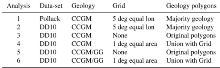
Table 4.Description of the various analyses undertaken. 5 deg eq lon; a grid with 5 degree spacing in longitude. 1 deg eq area; a grid with 1 degree spacing in longitude at the equator, but varying longi-tude at other latilongi-tudes to maintain an equal area. Majority Geology; the geology which takes up the greatest area inside the grid cell is ascribed to the whole grid cell. These and other aspects related to this table, including union, are described further in the text.
Analysis Data-set Geology Grid Geology polygons 1 Pollack CCGM 5 deg equal lon Majority geology 2 DD10 CCGM 5 deg equal lon Majority geology
3 DD10 CCGM None Original polygons
4 DD10 CCGM 1 deg equal area Union with Grid
5 DD10 CCGM/GG None Original polygons
6 DD10 CCGM/GG 1 deg equal area Union with Grid
3 Results
In Fig. 10, we plot the heat flow map of the world from our preferred analysis. The standard error (2 std. dev.) for the heat flow ascribed to each geological unit is presented in Fig. 11. We note that the error is highest for the young ocean estimates and the Glacier domains. Of course, these estimates of error are not useful locally; for example, some parts of Africa have no measurements. Therefore, like the value on the Global heat flow map being only indicative for that geology unit, likewise the error.
Results from the various cases examined are listed in Ta-ble 5. One can see that the raw global heat flow in each case varies from 35.8 to 36.7 TW, with our preferred analysis giv-ing a value of 36.7 TW. After the Stein and Stein (1992) SS-based young ocean estimate, one gets values ranging from 44.1 to 47.2 TW, with 47.2 TW for our preferred analysis; or 40.7 to 43.5 TW using the Parsons and Sclater (1977) PS-based estimate (43.4 TW for our preferred analysis). We note that the difference between estimates using only the raw data, and those using the SS half space model can vary between 7.8 and 11.1 TW, with a difference of 10.5 TW for our preferred analysis. We also note that using the SS and PS models leads to a difference of 3.4 to 3.8 TW (3.8 TW preferred analysis). Our preferred correction is between those of PS and SS, giv-ing a total heat flow value of 46.7 TW.
The preferred analysis can be divided into four compo-nents (see Table 6): (i) young oceans; (ii) the rest of the oceans and continents; (iii) the Glacier category; and (iv) the contribution from hot-spots. Each is next described in detail. 1. Our estimate for heat flow in young oceans produces 23.1 TW (128 mW m−2), compared to the 24.5 TW of Pollack et al. (1993) (PHJ93) (based on SS). Jaupart et al. (2007) (JLM07), whose value ofCwe have adopted, give 24.3 TW (the differences between our estimate and that of JLM07 arise from: (i) variations in the areas of geological units; (ii) the division of geologic time;
and (iii) the fact that ours covers oceanic crust out to 66.5 Ma while JLM07 extends out to 80 Ma), while Wei and Sandwell (2006) give a value of 20.4 TW. The PS model, with our area, leads to a young ocean heat flow estimate that is 2.8 TW less than that adopted here, while the SS model gives a value 1 TW greater. Con-sidering the PS-model estimate might be too low, it is clear that an uncertainty of∼2 TW is suggested by the alternative analyses listed above; our assumption that the error inCis±30 mW m−2Myr0.5at 2 standard de-viations, gives this component an error of±1.3 TW. 2. Estimates obtained for the rest of the oceans and
continental components depend upon: (i) the fun-damental assumption of a correlation between heat flow and geology; and (ii) the use of a 1 degree equal area grid to reduce the influence of clus-tering. Our preferred analysis predicts values of 13.8 TW/73 mW m−2(continents), 7.8 TW/66 mW m−2 (rest of oceans); for this component of the heat flow. This compares to 13.2 TW/65 mW m−2 (continents), 7.6 TW/56.4 mW m−2(rest of oceans) from PHJ93 and 14 TW/65 mW m−2 (continents), 4.4 TW/48 mW m−2 (>80 Ma) from JLM07. A significant percentage of the increased global heat flux in this study therefore arises due to this component, suggesting that heat flow values recently added to the global heat flow data-set have been, on average, slightly higher than earlier val-ues (as illustrated in the histogram of the raw data of Fig. 3b). This continues the slight upward trend in the estimate for global heat flux over recent years (see Ta-ble 4 PHJ93, and JLM07).
3. As described above, for the Glacier category we have used a value of 65 mW m−2 based on the depth to the Curie temperature found from undertaking a spec-tral analysis of aeromagnetic data (Maule et al., 2005), rather than the very small (2 to 5) measurements that fall within this category in the various analyses (the raw data gives heat flow estimates of 105 to 120 mW m−2for the various analyses – 113.5 mW m−2in the preferred anal-ysis). This gives a value of 0.9±0.3 TW. We note that using this alternative value for Antarctica (and Green-land), rather than the raw heat flow measurements, can make a difference of between 0.7 and 1.0 TW (0.7 TW in our preferred analysis). PHJ93 do not really address this issue while JLM07 include it in their total continen-tal area and effectively use the global average, which is 65.3 mW m−2. JLM07 include the error from this component in their total error estimate (for continents), which is 1 TW.
(a)
(b)
(c)
75 - 85
85 - 95
95 - 150
150 - 450 23 - 45
45 - 55
55 - 65
65 - 75
Fig. 10. (a)Map of the preferred global heat flux (mW m−2), utilising the underlying estimates for each geology category. Note that in
0 - 5
5 - 10
10 - 15
15 - 30
30 - 60
Fig. 11.Map of the estimated error in the preferred global heat flux (mW m−2). The error is based on the actual spread of heat flow values
for each geology category, with the exception of regions where the heat flow value is based on calculation (young oceanic crust) and the Glacier category (for more details see text). The mapped error does not include the component from hot-spots or the uncertainty in the area of geology polygons. We note that the largest error is related to the young oceanic crust and the glacier category.
JLM07 include a contribution for hot-spots in their anal-ysis, which they argue are not accounted for in their method. They estimate that this contribution is between 2 and 4 TW globally, based on Davies (1988) and Sleep (1990); with an error of ±1 TW. In our estimate for heat flow across young oceanic crust, we assume that the calibration measurements for the models have been selected to avoid hot-spots and, therefore, the effect of hot-spots is not included (thus a correction is needed). In contrast, we feel that hot-spot anomalies are included in the rest of the measurements on the ocean floor and continent. As a result, we only include a hot-spot cor-rection for the young oceanic domains, which is propor-tional to the surface area included in the young ocean estimate. We take a contribution of 1±0.33 TW. As mentioned above, some geology classes have very few heat flow measurements. We have looked at limiting our es-timates to only geology classes with: (i) at least 5; and (ii) at least 50 readings. Such a change has only a small effect on the final global estimate, of order ±0.3 TW (see Table 5). However, the random errors are reduced substantially by re-stricting the analysis to geology classes with at least 50 read-ings, although the errors in the young ocean estimates are much higher. This is because geology classes with less than 50 readings cover only a small percentage of Earth’s surface. Indeed, the remaining classes (i.e. with>50 readings) cover
>96% of Earth’s surface. Our preference is to ignore ge-ology classes with<50 readings. Our final preferred value is 46.7 TW, with an error of 2 TW (2 standard deviations). To be consistent with our error estimate of±2 TW we round 46.7 to 47 TW. This final preferred estimate is separated into the oceanic and continental realms in Table 7.
4 Discussion
Table 5.The total global surface heat flux from the various analyses undertaken. Note that the first row of results is from Pollack et al. (1993). Pollack is used as an abbreviation for the heat flow data-set, the geology and the method of using geology, used in Pollack et al. (1993). SS – Stein and Stein (1992); PS – Parsons and Sclater (1977); S. Join – spatial join; 1×1 long – 1 degree by 1 degree equal longitude grid; 1×1 area – 1 degree by 1 degree equal area grid; CCGM – Commission Geology Map of World (2000); GG – Global GIS (2003); DD10 – the data-set presented in this paper. The original version was provided by Laske and Masters (pers. comm.) and DD10 has only minor changes. See text for further explanation of terms and abbreviations used in table.
Case number from T able 4 Source of Heat Flo w Dataset
Geology Grid Ho
w is geology used? T otal Heat Flo w – (TW) – data based T otal Heat Flo w – with preferred young T otal Heat Flo w – with SS Dif ference between ra w data T otal Heat Flo w – with PS Dif ference between SS and PS T otal Heat Flo w with SS estimate b ut assum -Dif ference between original and assum-T otal Heat Flo w – with SS estimate (TW) T otal Heat Flo w – with SS estimate (TW) Antarctica and ocean ocean crust estimate (TW) and hot-spot based estimate (TW) and SS estimate (TW) based estimate (TW) estimates (TW) ing 65 mW m − 2for Antarctica (TW) ing 65 mW m − 2for Antarctica (TW) – excluding geologies with < 5 readings – excluding geologies with < 50 readings
PHJ93 Pollack Pollack 1×1 long Pollack avg 33.51 44.20 10.69
1 Pollack CCGM 5×5 long Pollack avg 36.25 44.06 7.81 40.68 3.38 43.08 0.98 43.39 43.42
2 DD10 CCGM 5×5 long Pollack avg 36.26 44.09 7.83 40.71 3.38 43.11 0.98 43.43 43.45
3 DD10 CCGM None S. Join 35.83 45.86 10.03 42.16 3.70 45.27 0.59 45.63 45.40
4 DD10 CCGM 1×1 area Union 36.14 47.06 11.08 43.35 3.71 46.46 0.60 46.75 47.03
5 DD10 CCGM + GG None S. Join 37.17 47.20 10.03 43.50 3.56 46.51 0.69 46.93 46.98
6 DD10 CCGM + GG 1×1 area Union 36.71 46.68 47.23 10.52 43.44 3.79 46.54 0.69 46.99 47.13
Table 6. The preferred analysis of Earth’s surface heat flux, broken down into five categories: (i) continents from data; (ii) oceanic crust
contribution by calculation (age<66.5 Myr); (iii) oceanic crust from data (age≥66.5 Myr); (iv) the glacier category; and (v) the hot-spot contribution. Columns of alternatives are also presented. “+1” signifies that this answer uses a 1-degree equal-area grid through a “union”, to reduce the influence of clustering. “50” means that only geology categories with at least 50 heat flow measurements were used in this answer. GG – Global GIS geology (Hearn et al., 2003); CCGM – CCGM geology (Commission for the Geological Map of the World, 2000); PHJ93 – result from Pollack et al. (1993) (breakdown calculated by combining information in their Tables 2 and 3); JLM07 – result from Jaupart et al. 2007). C510, C490, C430 – estimation using C values in Eq. (1) of 510, 490 and 430 mW m−2Myr0.5, respectively (SS – Stein and Stein (1992), whereCwas 510 mW m−2Myr0.5; PS – Parsons and Sclater (1977), whereCwas 430 mW m−2Myr0.5); WS – result for oceanic crust heat flow younger than 66 Myr from Wei and Sandwell (2006); 1983 T.S. – the 1983 Geological Time Scale (Palmer, 1983). Maule et al. (2005) is the estimate of Antarctica’s heat flow from Maule et al. (2005). Preferred total = 13.77 + 23.14 + 7.84 + 0.92 + 1.00 = 46.67 TW.
Continents (TW) Young Ocean Estimate (TW) Rest of Oceans (TW) Glacier (TW) Hot-spots (TW)
GG+CCGM+1; 50 13.8 CCGM, C510, 24.1 CCGM+1; 50 7.8 Raw data, CCGM +1 1.6 PHJ93 0.0
GG; 50 9.8 CCGM, C490, 23.1 CCGM; 50 8.3 Maule et al. (2005) 0.9 JLM07 3.0
CCGM+1; 50 13.0 CCGM, C430, 20.3 CCGM + 1 7.8 DD10 1.0
CCGM; 50 14.0 CCGM, C490, A (Eq. 3) 24.4 CCGM 7.8
GG+CCGM+1 13.7 PHJ93 (<66.4 Myr) 24.5 PHJ93 (>66.4 Myr) 7.6
GG 9.8 JLM07 (<80 Myr) 24.3 JLM07 (>80 Myr) 4.4
CCGM+1 13.0 WS (<66 Myr) 20.4
CCGM 14.2 CCGM, C490, 1983 T.S. 22.9
PHJ93 13.2
JLM07 14.0
Table 7. Summary of continental and oceanic heat flow from our preferred estimates.
Area Heat Flow Mean Heat Flow
(m2) (TW) (mW m−2)
Continent 2.073×10¹⁴ 14.7 70.9
Ocean 3.028×10¹⁴ 31.9 105.4
Global Total 5.101×10¹⁴ 46.7 91.6
0 40 80 120
0 5 10 15 20 25
Square Root of Age (Myr0.5)
M
e
an
H
e
at
F
lo
w
(
m
W
m
-2
)
Fig. 12. A plot of the average heat flow for each geology category
as a function of the square root of its mean age. There is a trend in the data, of decreasing mean heat flow with increasing age. If one excludes the very oldest datum (the Archean – which stretches over a very long geologic age) and the very youngest data (these cate-gories have very few measurements), there is a strong correlation. While the correlation of heat flow with geology could apply without a correlation between mean heat flow and age; the fact that such a correlation exists does lend some support that this fundamental as-sumption might have some merit. The correlation is strong enough (R2= 0.75) that it certainly seems better to take it into account than ignoring it.
4.1 The robustness of the fundamental correlation assumed
The fundamental correlation assumed by Pollack et al. (1993) (PHJ93) is that regions of similar geology have, on average, similar values for heat flow. From Table 3, one can see that the standard deviation on the mean values for various geology categories is very high, suggestive that this assump-tion is not useful. However, this is misleading. In Fig. 12, we plot the mean heat flow of different geology categories as a function of the square root of age, for all categories with greater than 50 measurements (the age for the Precambrian is hard to set; most of the measurements are likely to be in the Late Proterozoic, but we have no way of knowing the exact age distribution. As a result, the Precambrian cate-gory is excluded from our plot). Polyak and Smirnov (1968)
were among the first to suggest such a relationship, while Morgan (1985) pointed out that the relationship is weak. This weak relationship can be easily understood; although there is evidence of some decrease in heat production with age, the range of heat production within each age group is greater than the differences between age groups (Jaupart and Mareschal, 2003, 2007). Nevertheless we find that there is a clear correlation in the data, with the average heat flow de-creasing with inde-creasing age (R2= 0.75). This implies that there is some power in the correlation and that using such a methodology as an empirical estimator for un-sampled re-gions gives a better estimate (with slightly lower error) than a straightforward global average (as was done by Jaupart et al. (2007) (JLM07)). We remind readers that our assumption is that there is a correlation on average between geological category (not necessarily age) and heat flow. It should also be noted that our final estimate and that of JLM07 are simi-lar. The relationship between average age and heat flow for the continents with our data (excluding the Precambrian) is:
q=102−2.25√t (2) whereqrepresents heat flow (mW m−2)andtis the age
(mil-lions of years). We note that the thermo-tectonic age might lead to a further improved correlation. However, at the time of writing, such information was not available for the digital geologies used here.
Using this fundamental correlation, we find that the stan-dard error on each geology category is low, since our data-set contains a large number of individual measurements. As a consequence, the contribution of this to the final error is very small (note that the errors are area weighted, as is the global estimate). However, since the correlation (between geology and heat flow) is not perfect, the error in areas with very few measurements could potentially be higher. As a result, it is likely that our estimate for this component of the error is un-realistically low. Nonetheless, once one realises that: (i) the spread of continental and old oceanic heat flow values have a limited range; and (ii) the uncovered area is not that great (at least at a 5 degree sampling), it cannot be very large. The only way to confirm our prediction is to continue measuring heat flow, especially in currently un-sampled areas.
4.2 The raw heat flow data
4.2.1 Measurement techniques
that undertakes correction of heat flow measurements based upon climate and topography (note that such modern correc-tions are likely very rare in the data-set used here). While obtaining more accurate heat flow measurements is essential in constraining the global surface heat flux, we must accept that this will be a slow and expensive process. In the mean-time, as much as possible must be extracted from the mea-surements made to date.
4.2.2 Areal coverage of heat flow measurements
If we assume that the young ocean is well covered, since it is estimated from a model independent of our heat flow data, then at a 5 degree equal area grid sampling we find nearly 84% coverage; at 1 degree equal area spacing we have 53% coverage. The coverage is not very much more than PHJ93 (who had 62% coverage on a 5×5 degree grid), even though our data-set contains around 55% more heat flow measure-ments. This demonstrates that recent measurements added to the data-set were made in similar geographical locations to those in the data-set of PHJ93. Further measurements must be made in un-sampled regions to improve the reliability of global heat flow estimates.
4.3 Various analysis choices
We have undertaken various analyses using different meth-ods and data-sets (see Tables 4, 5 and 6). Such a range of analyses allows us to evaluate that: (i) the effect of in-cluding alternative geology is between 0.1 and 0.2 TW (see Table 5, 5th versus 7th row); (ii) not including the 1 degree grid increases clustering and leads to a decreased heat flow of ∼0.15 TW (Table 5, last two rows); (iii) increasing the threshold of points required to include a geology, as dis-cussed in Sect. 3, only changes the global heat flow slightly, but reduces that (small) component of the error; and (iv) the geological time scales used give heat flow estimates that dif-fer by 0.2 TW (see Table 6, 2nd column, 23.1–22.9 TW), which is very small (we utilised the 2004 Geological Time Scale (Gradstein et al., 2005) for our preferred estimate. The 1983 Geologic Time Scale (Palmer, 1983) was used for all other estimates). These analyses demonstrate that the final result is not sensitive to the details of these choices. In con-trast, the various analyses undertaken show that the young ocean estimate is a major contributor to the final error. 4.4 Hydrothermal correction in oceanic crust
It is well known that measurements of heat flow on young oceanic crust grossly underestimate the actual heat flow (Davis and Elderfield, 2004). This is due to relatively shal-low hydrothermal circulation. Theoretically, heat fshal-low is ex-pected to decline as the inverse square root of oceanic crustal age (Eq. 1). Indeed, this trend is observed in heat flow data over old oceanic crust. Therefore, in obtaining a complete
estimate of Earth’s surface heat flux, one must correct for hy-drothermal circulation in young oceanic crust, using Eq. (1). A value for the constant C must therefore be selected and one must know the distribution of ocean floor area as a function of age. We note also that the theoretical expression cannot apply at the very youngest age. We discuss these aspects in turn.
4.4.1 TheCconstant
As noted previously, estimates of the constantC vary; 430, 490 and 510 mW m−2Myr0.5, for PS, JLM07 and SS, re-spectively (note that these values are not strictly equiva-lent; JLM07 avoided hot-spots when calibrating data, but SS did not – in Table 5 we therefore do not include the hot-spot correction for the SS and PS cases. We have in-vestigated the influence of this constant on the total young ocean estimate by using all three values; the difference, bounded by the PS and SS values, is 3.8 TW. This is sig-nificant compared to other sources of uncertainty. Our pref-erence for C is the value of JLM07 (490 mW m−2Myr0.5),
although, as discussed in Sect. 2.4, we specify a larger un-certainty (30 vs. 20 mW m−2Myr0.5). This increased
uncer-tainty leads to a range of 2.6 TW, which is large, but less than the PS-SS range quoted above.
4.4.2 Area/age distribution
The estimate for heat flow in young oceanic crust is calcu-lated by multiplying the average heat flow for a certain age range by the total area for that age. As a consequence, varia-tions in the estimate of area for different age ranges could be significant. Table 1 lists the area of oceanic crust for CCGM geology. While using the listed area is the best approach, in this section we consider an alternative to get a sense of how significant this effect might be. JLM07, following Sclater et al. (1980) suggest that
dA
dτ =CA(1−τ/τm) (3)
where A is the area of oceanic crust (km2), τ is the age of the oceanic crust (years), and CA and τm are con-stants. In Fig. 13, we plot cumulative area as a function of age, using the 2004 Geology Timescale, finding that it is well fit by the above expression (R2= 0.98). We find
0.00E+00 1.00E+14 2.00E+14 3.00E+14
0 30 60 90 120 150 180
Age (Myr)
Ar
e
a
(
m
2)
Fig. 13.Cumulative area of oceanic crust (m2)as a function of age
(Ma). A least squares fit through the data for Eq. (3) is shown as a dark curve. We note that the data are reasonably well fit by such an expression, as pointed out originally by Sclater et al. (1980).
4.4.3 Correction in very young oceanic crust
The half space formulation has a singularity (infinite value) at the ridge axis (see Eq. 1). This is an integrable singularity so it causes no numerical problems. Davies et al. (2008) mod-elled the surface heat flow across a spreading ridge in a two-dimensional adaptive finite-element model. The model used a prescribed kinematic spreading upper surface to mimic the half space assumptions but avoided the unrealistic boundary condition at the ridge and had the resolution to numerically resolve the sharp variation. For a medium spreading rate of 5 cm yr−1, Davies et al. (2008) found that the heat flow curve
deviates from the half space curve at around 0.15 Myr and with an asymptotic value of just over 1 Wm−2. If these
con-ditions were the weighted average concon-ditions for all spread-ing ridges, the half-space model would overestimate the heat flow by around 0.1 TW. The overestimate would be locally greater for slower spreading ridges and less for faster spread-ing ridges. While this effect is not negligible, it is less than the estimated error and, hence, we have not considered it in our final error estimate.
4.5 Hydrothermal circulation on continents
Since hydrothermal circulation is critical to estimates of oceanic heat flux, it is sensible to enquire what role it might play on continents. JLM07 suggest that the contribution is likely to be small, given that the estimate for the entire Yel-lowstone system is around 5 GW, with similar values pre-dicted for the East African Rift. As stated by JLM07, it would require 200 “Yellowstones” to increase the continen-tal heat loss by 1 TW. Our current understanding suggests that the contribution from this component is less than the es-timated error.
4.6 Glacier category
The error arising from the Glacier category is potentially very large. As discussed earlier, our preference is a value of 65 mW m−2(Maule et al., 2005). The error bounds of the authors (∼24 mW m−2)leads to an uncertainty of∼0.3 TW (0.9×24/65), which is similar to our assumed error. We note that JLM07 estimate the error due to poor sampling to be around 1 TW; effectively this combines the error from: (i) the poor sampling discussed earlier; and (ii) the error aris-ing from the Glacier category. Our weighted combined esti-mate for these sources of error is 0.8 TW.
4.7 Combining statistical errors
Our final estimate of the total area weighted error is 2 TW. This is slightly higher than the estimate of PHJ93 since we have assumed more uncertainty arising from the young ocean estimate (and not ignored the uncertainty arising from poorly sampled categories – in this case arising from the “Glacier” category). It is 1 TW less than the error estimate of JLM07, even though our estimates of the error for individual com-ponents are similar. We estimate a contribution of: 1.3 TW (oceanic correction); 0.3 TW (Glacier category, which is re-lated to poor continental sampling in JLM07); 0.5 TW (rest of oceans); 0.3 TW (rest of continents – CCGM); 0.4 TW (rest of continents – GG); and 0.3 TW (hot-spots). Assum-ing that these error terms are independent and uncorrelated, the combined uncertainty is only 2 TW (not 4 TW if one in-correctly added the error contributions naively (e.g. forA= B+C, the errors should be combined1A2=1B2+1C2, not1A=1B+1C)). The biggest difference between our error and that of JLM07 is that we account for only 0.33 TW, compared to 1 TW, for the hot-spot correction.
4.8 Significance of result to thermal budget and thermal evolution models
Indeed, JLM07 argue that the initial temperature of the solid Earth was only∼200 K higher than the present-day. These figures therefore reveal an energy imbalance relating heat emerging at Earth’s surface and heat generated within Earth’s interior. There are, however, many hypotheses for how these diverging constraints can be satisfied, such as: (i) an in-creased CMB heat flux; and (ii) a delay between the gen-eration of heat in Earth’s interior and its arrival at the surface (see JLM07 for a discussion). Nonetheless, our revised es-timate of Earth’s surface heat flux only exacerbates this is-sue. Our result follows a recent trend of increasing global heat flow estimates, which makes the global “energy para-dox” described above (Kellogg et al., 1999) more difficult to understand.
5 Conclusions
Our revised estimate of Earth’s total surface heat flow is 47±2 TW, which is larger than previous investigations. This estimate was derived from an improved heat flow data-set, with 38 347 heat flow measurements and the methodologies of Geographical Information Science. Given the sparse and inhomogeneous nature of heat flow measurements globally (poor sampling in Antarctica, Greenland, Africa, Canada, Australia, South America and parts of Asia), there remain un-certainties in our estimate. In addition, models for hydrother-mal circulation in young oceanic domains exert a significant control on our final value. Our result follows a recent trend of increased estimates for Earth’s surface heat flow, thus posing difficulties for simple interpretations of heat sources in the mantle. Nonetheless, our estimate will provide a concrete boundary condition for future investigations of Earth’s ther-mal evolution.
Acknowledgements. We would like to acknowledge Gabi Laske and Guy Masters, Scripps Institution of Oceanography, UC San Diego, for providing us with the file of the enhanced heat flow measurements. We would also like to acknowledge all the indi-vidual hard work that has gone into collecting the raw data in the field, and in assembling this large data-base; including the efforts of Pollack and colleagues at University of Michigan, continuing with Gosnold and Panda, hosted at the University of North Dakota. We would like to acknowledge similarly the legions of hard work that has gone into making geology maps, and then to the groups that have assembled the maps into manageable digital files for ready use in GIS, especially the American Geological Institute (www.agiweb.org/pubs) and UNESCO/CCGM. All analyses were undertaken using the ESRI software ArcGIS 9.2 at the ArcInfo licence level. Jean-Claude Mareschal and Carol Stein are thanked for constructive and thorough reviews.
Edited by: J. C. Afonso
References
Beardsmore, G. R. and Cull, J. P.: Crustal Heat Flow, Cambridge University Press, Cambridge, 2001.
Buffett, B. A.: Estimates of heat flow in the deep mantle based on the power requirements for the geodynamo, Geophys. Res. Lett., 29, 1566, doi:1510.1029/2001GL014649, 2002.
Buffett, B. A.: The thermal state of Earth’s core, Science, 299, 1675–1677, 2003.
Christensen, U. R. and Tilgner, A.: Power requirement of the geodynamo from ohmic losses in numerical and laboratory dy-namos, Nature, 429, 169–171, doi:10.1038/nature02508, 2004. Commission for the Geological Map of the World: Geological Map
of the World at 1:25000000, 2nd Edn., UNESCO/CCGM, 2000. Davies, G. F.: Ocean bathymetry and mantle convection 1. Large
flow and hotspots, J. Geophys Res., 93, 10467–10480, 1988. Davis, E. and Elderfield, H. (Eds.): Hydrogeology of the oceanic
lithosphere, Cambridge University Press, Cambridge, 706 pp., 2004.
Davies, D. R., Davies, J. H., Hassan, O., Morgan, K., and Nithiarasu, P.: Adaptive finite element methods in geodynam-ics: Convection dominated mid-ocean ridge and subduction zone simulations, Int. J. Numer. Method. H., 18, 1015–1035, doi:10.1108/09615530810899079, 2008.
Gosnold, W. D. and Panda, B.: The Global Heat Flow Database of The International Heat Flow Commission, http://www.und.edu/ org/ihfc/index2.html (last access: 10 July 2007), 2002.
Gradstein, F. M., Ogg, J. G., and Smith, A. G.: A Geologic Time scale 2004, Cambridge University Press, Cambridge, 610 pp., 2005.
Hearn, P. J., Hare, T., Schruben, P., Sherrill, D., LaMar, C., and Tsushima, P.: Global GIS – Global Coverage DVD (USGS), American Geological Institute, Alexandria, Virginia, USA, 2003. Hernlund, J. W., Thomas, C., and Tackley, P. J.: A doubling of the post-perovskite phase boundary and structure of the Earth’s lowermost mantle, Nature, 434, 882–886, 2005.
Jaupart, C. and Mareschal, J.-C.: Constraints on crustal heat pro-duction from heat flow data, in: Treatise of Geochemistry, Vol. 3, The Crust, edited by: Rudnick, R. L., Elsevier Science Publish-ers, Amsterdam, 65–84, 2003.
Jaupart, C. and Mareschal, J.-C.: Heat flow and thermal structure of the lithosphere, in: Treatise on Geophysics, Vol. 6, edited by: Schubert, G., 217–252, Oxford, Elsevier Ltd., 2007.
Jaupart, C., Labrosse, S., and Mareschal, J.-C.: Temperatures, heat and energy in the mantle of the Earth, in: Treatise on Geophysics, Vol. 7, Mantle Convection, edited by: Bercovici, D., Elsevier, 253–303, 2007.
Kellogg, L. H., Hager, B. H., and van der Hilst, R. D.: Composi-tional stratification in the deep mantle, Science, 283, 1881–1884, 1999.
Korenaga, J.: Energetics of mantle convection and the fate of fossil heat, Geophys. Res. Lett., 30, 1437, doi:10.1029/2002GL016179, 2003.
Labrosse, S., Hernlund, J. W., and Coltice, N.: A crystallizing dense magma ocean at the base of the Earth’s mantle, Nature, 450, 866– 869, doi:10.1038/nature06355, 2007.
Lee, W. H. K. and Uyeda, S.: Review of heat flow data, in: Terres-trial Heat Flow, edited by: Lee, W. H. K., Geophys. Mono., 8, AGU, Washington, D.C., 87–190, 1965.
Lyubetskaya, T. and Korenaga, J.: Chemical composition of Earth’s primitive mantle and its variance: 2. Implications for global geodynamics, J. Geophys. Res., 112, B03212, doi:10.1029/2005JB004224, 2007a.
Lyubetskaya, T. and Korenaga, J.: Chemical composition of Earth’s primitive mantle and its variance: 1. Method and results, J. Geo-phys. Res., 112, B03211, doi:10.1029/2005JB004223, 2007b. Maule, C. F., Purucker, M. E., Olsen, N., and Mosegaard, K.: Heat
flux anomalies in Antarctica revealed by satellite magnetic data, Science, 309, 464–467, 2005.
McDonough, W. and Sun, S.: The composition of the Earth, Chem. Geol., 120, 223–253, 1995.
Morgan, P.: Crustal radiogenic heat production and the selective survival of ancient continental crust, J. Geophys. Res., Supple-ment, 90, C561–C570, 1985.
Nimmo, F., Price, G. D., Brodholt, J., and Gubbins, D.: The influ-ence of potassium on core and geodynamo evolution, Geophys. J. Int., 156, 363–376, 2004.
Palme, H. and O’Neill, H. S. C.: Composition of the Primitive Man-tle, in: Treatise on Geochemistry, Vol. 2, The Mantle and Core, edited by: Carlson, R. W., Elsevier Scientific Publishers, Ams-terdam, 1–38, 2003.
Palmer, A. R.: Decade of North American Geology (DNAG), Geo-logic time scale, Geology, 11, 503–504, 1983.
Parsons, B. and Sclater, J.: An analysis of the variation of ocean floor bathymetry and heat flow with age, J. Geophys. Res., 82, 803–827, 1977.
Pollack, H. N., Hurter, S. J., and Johnson, J. R.: Heat-Flow from the Earths Interior – Analysis of the Global Data Set, Rev. Geophys., 31, 267–280, 1993.
Polyak, D. G. and Smirnov, Y. A., Relation between terrestrial heat flow and tectonics of the continents, Geotectonics, 4, 205–213, 1968.
Rudnick, R. and Fountain, D.: Nature and composition of the continental-crust – A lower crustal perspective, Rev. Geophys., 33, 267–309, 1995.
Sclater, J. G., Jaupart, C., and Galson, D.: The heat flow through oceanic and continental crust and the heat loss of the Earth, Rev. Geophys. Space Phys., 18, 269–311, 1980.
Shapiro, N. M. and Ritzwoller, M. H.: Inferring surface heat flux distributions guided by a global seismic model: particular ap-plication to Antarctica, Earth Planet. Sci. Lett., 223, 213–224, 2004.
Sharpe, H. N. and Peltier, W. R.: Parameterized mantle convection and the Earth’s thermal history, Geophys. Res. Lett., 5, 737–740, 1978.
Slagstad, T., Balling, N., Elvebakk, H., Midttømme, K., Ole-sen, O., OlOle-sen, L., and Pascal, C.: Heat-flow measurements in Late Palaeoproterozoic to Permian geological provinces in south and central Norway and a heat-flow map of Fennoscandia and the Norwegian-Greenland Sea, Tectonophysics, 473, 341–361, 2009.
Sleep, N. H.: Hotspots and mantle plumes : some phenomenology, J. Geophys. Res., 95, 6715–6736, 1990.
Stein, C. A. and Stein, S.: A model for the global variation in oceanic depth and heat flow with lithospheric age, Nature, 359, 123–129, 1992.
Stein, C. A. and Von Herzen, R. P.: Potential effects of hydrother-mal circulation and magmatism on heat flow at hotspot swells, in: Plates, Plumes and Planetary Processes, edited by: Foulger, G. R. and Jurdy, D. M., Geol. Soc. Am. Sp. Paper, 430, 261–274, doi:10.1130/2007.2430(13), 2007.
Wei, M. and Sandwell, D.: Estimates of heat flow from Cenozoic seafloor using global depth and age data, Tectonophysics, 417, 325–335, 2006.