www.biogeosciences.net/11/7369/2014/ doi:10.5194/bg-11-7369-2014
© Author(s) 2014. CC Attribution 3.0 License.
Components of near-surface energy balance derived from satellite
soundings – Part 2: Noontime latent heat flux
K. Mallick1, A. Jarvis2, G. Wohlfahrt3,8, G. Kiely4, T. Hirano5, A. Miyata6, S. Yamamoto7, and L. Hoffmann1
1Environmental Research and Innovation (ERIN), Luxembourg Institute of Science and Technology (LIST), L4422, Belvaux,
Luxembourg
2Lancaster Environment Centre, Lancaster University, Lancaster LA1 4YQ, UK 3Institute of Ecology, University of Innsbruck, 6020 Innsbruck, Austria
4Hydrology Micrometeorology and Climate Investigation Centre, Department of Civil and Environmental Engineering,
University College Cork, Cork, Ireland
5Division of Environmental Resources, Research Faculty of Agriculture, Hokkaido University, Hokkaido, Japan 6National Institute for Agro-Environmental Sciences, Tsukuba, Japan
7Graduate School of Environmental Science, Okayama University Tsushimanaka 3-1-1, Okayama 700-8530, Japan 8European Academy of Bolzano, 39100, Bolzano, Italy
Correspondence to:K. Mallick (kaniska.mallick@gmail.com)
Received: 27 March 2014 – Published in Biogeosciences Discuss.: 4 June 2014
Revised: 31 October 2014 – Accepted: 10 November 2014 – Published: 22 December 2014
Abstract. This paper introduces a relatively simple method for recovering global fields of latent heat flux. The method focuses on specifying Bowen ratio estimates through exploit-ing air temperature and vapour pressure measurements ob-tained from infrared soundings of the AIRS (Atmospheric Infrared Sounder) sensor onboard NASA’s Aqua platform. Through combining these Bowen ratio retrievals with satel-lite surface net available energy data, we have specified es-timates of global noontime surface latent heat flux at the 1◦×1◦scale. These estimates were provisionally evaluated against data from 30 terrestrial tower flux sites covering a broad spectrum of biomes. Taking monthly average 13:30 data for 2003, this revealed promising agreement between the satellite and tower measurements of latent heat flux, with a pooled root-mean-square deviation of 79 W m−2, and no significant bias. However, this success partly arose as a prod-uct of the underspecification of the AIRS Bowen ratio com-pensating for the underspecification of the AIRS net avail-able energy, suggesting further refinement of the approach is required. The error analysis suggested that the landscape level variability in enhanced vegetation index (EVI) and land surface temperature contributed significantly to the statistical metric of the predicted latent heat fluxes.
1 Introduction
7370 K. Mallick et al.: Components of near-surface energy balance
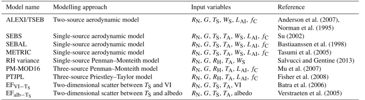
sensing data have been developed and used to evaluate the spatio-temporal behaviour of evaporation for field (Tasumi et al., 2005), regional (Bastiaanssen et al., 1998; Su, 2002; Mu et al., 2007; Mallick et al., 2007; Jang et al., 2010) and continental scales (Anderson et al., 2007; Sahoo et al., 2011). The methods employed thus far can be categorised based on the various approaches followed to determineE. The most common approach centres on assuming a physical model of evaporation given many of the variables required to com-pute evaporation using these models are available directly as satellite products (e.g. land surface temperature, vegeta-tion index, albedo) (Choudhury and Di Girolamo, 1998; Mu et al., 2007, 2011). The Priestley–Taylor (Priestley and Tay-lor, 1972)-based model for estimating monthly globalE re-lies on constraining the Priestley–Taylor parameter with me-teorological and satellite-based biophysical variables (frac-tional vegetation cover, green canopy fraction, vegetation in-dex, etc.) (Fisher et al., 2008; Vinukollu et al., 2011). In con-trast, a number of studies have also tried to resolveE indi-rectly by estimating the evaporative fraction from the rela-tionship between satellite-derived albedo, vegetation indices and land surface temperature (Verstraeten et al., 2005; Batra et al., 2006; Mallick et al., 2009). More recently, Salvucci and Gentine (2013) proposed a novel method for determin-ing E based on minimising the vertical variance of rela-tive humidity while simultaneously estimating water vapour conductance and E. A list of the widely used global- and regional-scale satellite-basedEmodels is listed in Table 1.
What is common to all these approaches is that they rely to a greater or lesser extent on parameterisation of surface char-acteristics in order to derive the estimates of E and there-fore the products from these approaches are conditional on these parameterisations. For example, in schemes which ex-ploit the Penman–Monteith equation, both the aerodynamic and surface resistance terms require some form of calibration of surface characteristics, often involving vegetation indices, whether empirically (Mu et al., 2007) or through linking to photosynthesis (Anderson et al., 2008). This is obviously a confounding factor when one attempts to use these data to evaluate surface parameterisations in weather, climate and hydrological models, particularly when the models we wish to evaluate may contain very similar model descriptions for
E. What is required, therefore, are methods for derivingE
estimates from satellite data that do not rely unduly on sur-face parameterisations, and thus they become a valid and valuable data source for model evaluation. One approach that appears to fulfil this requirement is whereλE is estimated from satellite data as a residual term in the energy balance equation (Tasumi et al., 2005; Mallick et al., 2007). However, this approach suffers from the effects of error propagation because all errors, including any lack of observed closure of the regional energy budget, are lumped into the estimate of
λE(Foken et al., 2006). From this we can see that something more akin to a satellite “observation” would be attractive.
Global polar-orbiting sounders like AIRS (Atmospheric Infrared Sounder) provide profiles of air temperature and rel-ative humidity at different pressure levels from the surface to the upper troposphere, along with several other geophysical variables (for example, surface temperature, near-surface air temperature, precipitable water, cloudiness, surface emissiv-ity, geopotential height). Profile information like this points to the possibility of exploring gradient-based methods such as Bowen ratio (Bowen, 1926) to produce large-scale esti-mates ofE. Despite having been used to refine estimate of near-surface air temperature over the oceans (e.g. Hsu, 1998), the use of Bowen ratio methods in conjunction with satel-lite sounder data somewhat surprisingly appears to have been overlooked as a method for estimatingE. The reasons for this are probably twofold. Firstly, the resolutions of the tempera-ture and humidity retrievals are assumed to be inadequate for differential methods like this. Secondly, there can be reserva-tions over the applicability of the underlying assumpreserva-tions of gradient methods on this scale. Although these appear valid concerns, there are also important counter-arguments to con-sider. Firstly, the degree of signal integration going on at the scale of the satellite sounding should help relax the require-ment on signal resolution. Sounders integrate signal horizon-tally over scales of thousands of square kilometres and hence benefit from strong spatial averaging characteristics in the measurement, despite suffering from ambiguities in the ver-tical integration of signal. However, this later drawback is aided by an effectively large sensor separation in the verti-cal (Thompson and Hou, 1990). Secondly, studies over both ocean and land indicate that the Bowen ratio method can be relatively robust under non-ideal conditions (Tanner, 1961; Todd et al., 2000; Konda, 2004). Given the potential bene-fits of having non-parametric estimates ofEat the scales and spatial coverage offered by the satellites, we argue that the possibility of using sounder products within a Bowen ratio framework merits investigation.
This paper presents the development and evaluation of 1◦×1◦AIRS sounder–Bowen ratio-derived latent heat flux,
λE. We focus on terrestrial systems because of the availabil-ity of an extensive tower-based flux measurement network against which we can evaluate the various satellite-derived components.
2 Methodology
2.1 Bowen ratio methodology
The Bowen ratio (β) is the ratio of sensible,H (W m−2), to
latent,λE(W m−2), heat flux (Bowen, 1926), β= H
λE, (1)
instan-Table 1.A list of satellite-based evapotranspiration models.
Model name Modelling approach Input variables Reference
ALEXI/TSEB Two-source aerodynamic model RN,G,TS,WS,LAI,fC Anderson et al. (2007),
Norman et al. (1995)
SEBS Single-source aerodynamic model RN,G,TS,TA,WS,LAI,fC Su (2002)
SEBAL Single-source aerodynamic model RN,G,TS,TA,WS,LAI,fC Bastiaanssen et al. (1998) METRIC Single-source aerodynamic model RN,G,TS,TA,WS,LAI,fC Tasumi et al. (2005)
RH variance Single-source Penman–Monteith model RN,G,RH,TA,WS Salvucci and Gentine (2013)
PM-MOD16 Three-source Penman–Monteith model RN,G,RH,TA,LAI,fC Mu et al. (2007) PTJPL Three-source Priestley–Taylor model RN,G,RH,TA,LAI,fC Fisher et al. (2008) EFVI−TS Two-dimensional scatter betweenTSand VI RN,G,TS,TA, VI Batra et al. (2006)
EFalb−TS Two-dimensional scatter betweenTSand albedo RN,G,TS,TA, albedo Verstraeten et al. (2005)
RN: net radiation;G: ground heat flux;TS: land surface temperature; VI: vegetation index;LAI: leaf area index;fC: fractional vegetation cover;TA: air temperature;RH: relative humidity;WS: wind speed.
taneous energy balance of the plane across whichH andλE
are being considered is given by
8=RN−G=λE+H, (2)
where8(W m−2) is known as the net available energy,RN
(W m−2) is the net radiation across that plane andG(W m−2) is the rate of system heat accumulation below that plane; then, combining Eqs. (1) and (2), one gets
λE= 8
1+β. (3)
Therefore, if 8 andβ are available, λE can be computed (Dyer, 1974). The estimation of8from satellite data is cov-ered in a companion paper (Mallick et al., 2014).βwas esti-mated as follows.
H andλEare assumed to be linearly related to the verti-cal gradients in air temperature and partial pressure of water vapour,∂T /∂zand∂p/∂z, through assuming similarity in the pathways for the two fluxes.
λE=ρλεkE ∂p
∂z (4a)
and
H=ρcPkH ∂T
∂z, (4b)
whereεis the ratio of the molecular weight of water vapour to that of dry air,ρ is air density (kg m−3),cpis air specific
heat (J kg−1K−1), andkE andkH are the effective transfer
coefficients for water vapour and heat, respectively (m s−1) (Fritschen and Fritschen, 2005). If heat and water vapour oc-cupy the same transfer pathway and mechanism through a plane, thenkE≈kH(Verma et al., 1978) and Eqs. (1) and (4)
reduce to
β= cP λε
∂T
∂p, (5)
suggestingβcan be estimated from the relative vertical gra-dient inT andp(Bowen, 1926). In the turbulent region of the atmosphere, eddy diffusivities for all the conserved scalars are generally assumed equal because they are carried by the same eddies and, therefore, are associated at source (Swin-bank and Dyer, 1967). There is evidence to suggestkH is
greater thankE under stable (early morning and late
after-noon) conditions when heat gets transferred more efficiently than the water vapour (Katul et al., 1995) and when the ef-fects of lateral advection of heat are significant (Verma et al., 1978). For non-neutral atmospheric conditions the turbu-lent efficiency for transporting water vapour is more than that for heat (Katul et al., 1995), and under such conditionskE
is greater thankH. For the near-convective conditions (early
to mid-afternoon) the ratio of kH to kE is unity (Katul et
al., 1995).
AIRS soundings forT andp are available for a range of pressure levels in the atmosphere (Tobin et al., 2006). As-suming the lowest available two pressure levelsp1,2 occur
within a region of the planetary boundary layer within which Eqs. (4a) and (b) hold, then a finite difference approximation of Eq. (5) gives
β= cP λε
(T1−T2+Ŵ) (p1−p2)
, (6)
whereŴ accounts for the adiabatic lapse rate inT, which in this case will be significant. Here we specifyŴfollowing Eq. (6.15) in Salby (1996), which when rearranged gives
Ŵ=ln(T2/T1) Ŵd
ln(p2/p1) κ
, (7)
whereŴdis the dry adiabatic lapse rate (∼9.8 K km−1) and κis the ratio of the specific gas constant (J kg−1K−1) to the isobaric specific heat capacity (J kg−1K−1).
7372 K. Mallick et al.: Components of near-surface energy balance
observations of the vertical gradients are dominated by ver-tical transport, and hence the effects of advective fluxes are minimal. This is a real problem in traditional, small-scale, near-surface applications because the length of the vertical flux path being sampled is similar to that of many of the turbulent fluxes involved in near-surface heat and mass ex-change. As a result, the observed vertical gradient can be-come partially distorted by the lateral advection of heat and water vapour (Wilson et al., 2001). In contrast, the satel-lite sounding data sample a radically different space with a horizontal extent varying from 0.5 to 1◦. In this prelimi-nary investigation we have opted to use the AIRS sounding data where the horizontal footprint is 1◦×1◦ (or approxi-mately 100 km×100 km). For the vertical profile we exploit the 1000 and 925 mb pressure level soundings, correspond-ing to heights of approximately 10 and 500 m. Therefore the vertical scale is nearly 3.5 orders of magnitude smaller than the horizontal. Although advective fluxes occur across a range of scales in space, they are slow relative to the verti-cal exchange on these sverti-cales and hence should tend to distort the vertical gradient to a lesser extent than traditional Bowen towers.
The second assumption is related to the first in that the lateral advective fluxes become particularly important when the underlying land surface is heterogeneous because lateral import of heat or mass into the observation space from ad-jacent land patches will again distort the gradient measure-ments. For the reasons expressed above on the relative scales of the vertical and horizontal footprint of the sounding obser-vations, such “edge effects” should be diminished, although it is important to appreciate that the landscape heterogene-ity is likely to increase with scale. Therefore, although the satellite-based method we are proposing shows promise as an observation platform, relating these observations to unique surface characteristics is likely to be problematic (despite an attempt being made (Fig. 6) to explain the retrieval errors in light of the vegetation biophysical heterogeneity).
The final assumption is that the land–atmosphere system is in some form of dynamic equilibrium so that the vertical gradients representing vertical fluxes and changes in storage are trivial. The soundings we utilise are for a 13:30 over-pass time. Although not universally so, the turbulent bound-ary layer tends to be approaching its most mature by this time of day and the average depth of the turbulent boundary layer should extend well beyond the 925 mb level (Fisch et al., 2004). Therefore, the steady-state assumption implicit in Bowen ratio methods (Fritschen and Simpson, 1989) is prob-ably closest to being fulfilled. That said, the development of the turbulent boundary layer depends on the nature of the (radiative) forcing it is experiencing and there may be many circumstances when it is still evolving at the 13:30 overpass time. Although this has implications for the steady-state as-sumption, it probably has bigger implications for the assump-tion that the boundary layer has developed beyond the lowest
two available soundings and hence can be considered fully turbulent.
Although the system we are sampling is not the con-stant flux region near the surface, in effect we have a sur-face source region (sampled by the 1000 mb sounding) ex-changing with a well-mixed volume (sampled by the 925 mb sounding). The flux exchange between these two should be approximately linear and equivalent in the concentration dif-ferences between the two, providing we are near dynamic equilibrium (i.e. the turbulent boundary layer is not grow-ing/contracting excessively) and that additional fluxes into and out of the boundary layer (including phase changes) are small relative to the surface sourced fluxes of heat and water vapour.
The principle difficulty as far as we can ascertain is the ef-fect of phase changes associated with cloud formation, pro-ducing latent warming of the boundary layer whilst remov-ing water vapour. Providremov-ing this happens above the 925 mb sounding, we anticipate it being less of a problem, but if it happens below this level then clearly this is problematic. Of course, this also impacts on the estimation of the net avail-able energy.
The reliability of the estimates ofβ also depends on the accuracy and resolution of the measurements of the temper-ature and humidity gradients. The AIRS products are quoted as having resolutions and accuracies of±1 K km−1forT and
±10 % km−1forp(Aumann et al., 2003; Tobin et al., 2006). Given Bowen ratio studies are invariably applied to small sensor separations of the order of metres, and at the point scale, precisions of±0.01◦C for temperature and±0.01 kPa for vapour pressure are required (Campbell Scientific, 2005), making the AIRS sensitivities appear untenable. However, as mentioned above, the effective sensor separation of the order of hundreds of metres allied to the sounding integrating at the 10 000 km2scale should help lift these restrictions. There are missing data segments in the AIRS sounder profiles, which are particularly prominent at high latitudes, where presum-ably it is difficult to profile the atmosphere relipresum-ably near the surface, and over the mountain belts, where the lower pres-sure levels are intercepted by the ground.
A general sensitivity–uncertainty analysis was carried out to assess the propagation of uncertainty through the cal-culation scheme onto the estimates of λE (see Mallick et al., 2014, for details).
2.2 Satellite data sources
the daily data of each grid box. The monthly merged prod-ucts have been used here because the infrared retrievals are not cloud-proof and the monthly products gave decent spatial cover in light of missing cloudy-sky data. The data products were obtained in hierarchical data format (HDF4) with as-sociated latitude–longitude projection from NASA’s Mirador data holdings (http://mirador.gsfc.nasa.gov/). These data sets included all the meteorological variables required to realise Eqs. (6) and (7).
2.3 Tower evaluation data
The satellite estimates of β, λE and H were evaluated against 2003 data from 30 terrestrial FLUXNET eddy co-variance towers (Baldocchi et al., 2001) covering 7 differ-ent biome classes. These tower sites were selected to cover a range of hydro-meteorological environments in South Amer-ica, North AmerAmer-ica, Europe, Asia, Oceania and Africa. A comprehensive list of the site characteristics and the site lo-cations are given in a companion paper (Mallick et al., 2014), which describes the specification of the satellite net available energy used here.
Eddy covariance has largely replaced gradient-based methods like the Bowen ratio as the preferred method for tower measurements of terrestrial water vapour and sensi-ble heat flux. Because eddy covariance is not a gradient method it is an attractive source of evaluation data. Sen-sible and latent heat flux measurements were used as re-ported in the FLUXNET data base; in other words no cor-rections for any lack in energy balance closure (Foken, 2008; Wohlfahrt et al., 2009) were applied. The spatial scale of the tower eddy covariance footprint is of the order of∼1 km2 and is hence on a scale approximately 4 orders of magnitude smaller than the 10 000 km2satellite data, which obviously has implications in heterogeneous environments (see above). The most important implication for spatial heterogeneity in the present context is that, in addition to complicating com-parison with tower data, relating these observations to unique surface characteristics is likely to be problematic.
3 Results
3.1 Bowen ratio – evaporative fraction evaluation Figure 1a shows the global distribution of annual average, 13:30 h estimates forβ for the year 2003 derived using the sounder method. The missing data segments are due to two data rejection criteria, one of which is already mentioned in Sect. 2.1. We have additionally imposed our own data re-jection for β when there is reversal of the vertical vapour pressure gradient under high radiative load. This condition is often encountered in hot, arid settings when large-scale ad-vection causes the assumptions behind Bowen ratio method-ology to become invalid (Rider and Philip, 1960; Perez et al., 1999). This condition was particularly prevalent over
a. b.
c. d.
Bowen ratio β (W m Net available energy, Φ Latent heat flux, E (Wm
Figure 1. Global fields of yearly average 13:30 derived from AIRS sounder observations for 2003. (a) Bowen ratio β
(W m−2/W m−2).(b)Net available energy,8(Wm−2).(c)Latent heat flux,λE(Wm−2).(d)Sensible heat flux,H(Wm−2). Missing data are marked in grey.
Australia in summer 2003 (Feng et al., 2008) and hence this region is not covered particularly well.
The first thing to note from Fig. 1a is that there is a clear land–sea contrast with β being relatively low and uniform over the sea as expected. The values ofβover the oceans are in the region of 0.1, in line with commonly quoted figures for the sea (Betts and Ridgway, 1989; Hoen et al., 2002). Over the tropical forest regions of Amazonia and the Congo, β
is in the range of 0.1 to 0.3, which also compares with val-ues reported for these areas (da Rocha et al., 2004, 2009; Russell and Johnson, 2006). The more arid areas are also clearly delineated. Although somewhat variable, the Sahara gives a range of 1.5–3.5, which corresponds to the results of Kohler et al. (2010) and Wohlfahrt et al. (2009) for the Mojave Desert. The South American savanna gives a range between 0.5 and 1, which corresponds to values reported by Giambelluca et al. (2009). One notable feature is the ho-mogeneity of theβ fields over the Americas in contrast to the heterogeneity over Eurasia. The year 2003 was associ-ated with widespread drying over Europe (Fink et al., 2004), which may explain this feature.
7374 K. Mallick et al.: Components of near-surface energy balance
valuation of the radiosonde derived evaporative fraction, Λ. This produces a Λ(radiosonde) = 1.12(±0.24)Λ(tower)
.4
.6
.8
1
.4
.6
.8
1
tower
r
ad
ios
on
d
e
Figure 2. Evaluation of the radiosonde-derived evaporative fraction, 3. This produces a correlation of 0.69 (R2=0.48) and a regression line (solid black line) of 3(radiosonde) =
1.12(±0.24)3(tower)−0.08(±0.16).
current manuscript. We have elected to evaluate β in terms of evaporative fraction (3) (=(1+β)−1) (Shuttleworth et
al., 1989) because, unlike β,3 is bounded and more lin-early related to the tower fluxes from which it is derived (λE=38, cf. Eq. 3). Figure 2 shows the relationship be-tween the radiosonde- and tower-derived estimates of3and reveals a fair degree of correspondence between the two. This analysis produces a significant and modest correlation (r=
0.69±0.101), reasonably low RMSE (0.11) and mean abso-lute percent deviation (14 %) between radiosonde-derived3
and tower-observed3.
Figure 3a shows the relationship between the satellite-and tower-derived estimates of3. The evaluation in Fig. 3a reveals a significant correlation (r=0.34±0.061) between
3(satellite) and3(tower), albeit one corrupted by significant variability. This is to be expected givenβis defined as a ra-tio of either four uncertain soundings (for the satellite) or two uncertain fluxes (for the tower). Assuming both measures are co-related through some “true” intermediate-scale variable, then the slope and intercept of the regression relationship be-tween the AIRS- and tower-observed3are 0.31 (±0.02) and 0.49 (±0.04), respectively.
The sensitivity analysis results are given in Table 2 and show a differentially higher sensitivity to the vapour pressure observations than for temperature, and a standard deviation of 0.11 on the estimates of3(satellite), although these results are dependent on the level of the input data given the inverse nonlinearity in Eq. (6).
1All uncertainties are expressed as±one standard deviation un-less otherwise stated.
3.2 Latent and sensible heat evaluation
Figures 1b and 3b show the geographical distribution of the average noontime net available energy and its evalua-tion for the year 2003 taken from Mallick et al. (2014). The corresponding geographical distributions ofλEandH
are shown in Fig. 1c and d. Figure 3c shows the relation-ship between the satellite and towerλEfor all 30 evaluation sites. This gives an overall correlation ofr=0.75(±0.04). Assuming both the tower and satellite data are linearly co-related, linear regression between the satellite and tower
λE gaveλE(satellite) =0.98(±0.02)λE(tower) (offset not significant) with a root-mean-square deviation (RMSD) of 79 W m−2 (see Fig. 3c). The biome-specific statistics for
λEare given in Table 3, which reveals correlations ranging from r=0.41(±0.22)(SAV, savanna) to r=0.76(±0.10)
(ENF, evergreen needleleaf forest), RMSD ranging from 61 (MF) to 141 (SAV) W m−2and regression gains ranging from 0.85(±0.08) (CRO, crops) to 2.00(±0.28) (SAV). Higher correlations (r=0.65−0.76) were evident over the forest sites where the tower height ranged from 40 to 65 m, fol-lowed by moderate correlation over crops (CRO) and grasses (GRA) (r=0.59−0.67) with tower height of 5–10 m (Ta-ble 3). Similarly, the slope of the correlation was close to unity for the forests and less than unity for CRO and GRA (Table 3) (Fig. 4). The only exception was found in savanna (SAV), which showed significant overestimation and low cor-relation (Table 3, Fig. 4; reasons discussed later).
The relationship between the satellite and tower H
for all 30 evaluation sites is shown in Fig. 3d. Here,
r=0.56(±0.05) and the regression between the satellite-predicted and tower-observedH produced a regression line of H(satellite)=0.59(±0.02)H(tower) with an RMSD of 77 W m−2 for the pooled data. Again, the biome-specific statistics for H are given in Table 3 and reveal corre-lations ranging from 0.43(±0.15) (GRA) to 0.79(±0.11)
(CRO), RMSD ranging from 52 (CRO) to 149 (SAV) W m−2 and regression gains ranging from 0.45(±0.05) (SAV) to 0.93(±0.06) (CRO). Figure 5 shows some examples of monthly time series ofλEfor both the satellite and the tow-ers for a range of sites. This reveals that the seasonality in
λE(tower) is relatively well captured inλE(satellite) in the majority of cases with the exception of Vielsalm, Tsukuba and Skukuza. Therefore, the individual site statistics given in Table 3 largely reflect the seasonality in the tower data.
The sensitivity–uncertainty results forλEare given in Ta-ble 2, revealing a standard deviation on the estimate ofλE
from the ensemble of 60 W m−2and significant sensitivity to the range of inputs used to calculate bothβand8.
4 Discussion
a. b.
c. d.
Evaporative fraction, Λ. Here, the solid
Λ(satellite) = 0.31(±0.02)Λ(tower) + 0.4λ(±0.04) Net available energy, Φ. He
line denotes Φ(satellite) = 0.λ0 (±0.03)Φ(tower) – E.
○ ◊ □
0 .25 .50 .75 1.0
0 .25 .50 .75 1.0
tower
s
a
te
ll
it
e
0 200 400 600
0 200 400 600
tower (W m
-2)
s
a
te
ll
it
e
(
W
m
-2
)
0 200 400 600 0
200 400 600
E tower (W m
-2)
E
s
a
te
ll
it
e
(
W
m
-2
)
0 200 400
0 200 400
H tower (W m
-2)
H
s
a
te
ll
it
e
(
W
m
-2
)
Figure 3. The evaluation of the AIRS-derived monthly 13:30 surface flux components against their tower equivalent.(a)Evaporative fraction,3. Here, the solid regression line denotes3(satellite)=0.31(±0.02)3(tower)+0.49(±0.04).(b)Net available energy,8. Here, the solid regression line denotes8(satellite)=0.90(±0.03)8(tower)−2.43(±8.19)(see Mallick et al., 2014).(c)Latent heat flux,λE. (d)Sensible heat flux,H. For regression statistics see Table 3. The 1:1 line is shown for reference.
(+EBF;×MF;GRA;∗CRO;∇ENF;♦DBF;SAV)
EBF: evergreen broadleaf forest; MF: mixed forest; GRA: grassland; CRO: cropland; ENF: evergreen needleleaf forest; DBF: decid-uous broadleaf forest; SAV: savanna
on the estimation ofβand hence3. From Table 2 we see the ensemble distribution of 3 has a significant negative skew due to taking the inverse of the noise onp1andp2(cf. Eq. 6).
As a result, there will be a tendency to overspecify3from the sounding data given the “true” value will be less than the mode. Both the likelihood and the magnitude of this over-specification will increase as p1−p2→0 (i.e. as3→0)
because of a decreasing signal-to-noise ratio. This explains why3(satellite) and3(tower) diverge as3→0. An addi-tional reason for this divergence is provided by the fact that
H(satellite) < H(tower) due to the effects of warm air en-trainment (see later).
The retrieval ofλEdepends heavily on 8, hence the in-crease in the satellite-to-tower correlation seen forλE rela-tive to3. Indeed,3is a relatively stable characteristic within site, and so the variance ofλEis dominated by seasonal and diurnal variations inRN and8(da Rocha et al., 2004;
Ku-magai et al., 2005). For a detailed discussion of the efficacy of the satellite-derived values of8 we have used here, the
reader is referred to Mallick et al. (2014). To summarise, in comparing the satellite-derived 8with the towerH+λE, Mallick et al. (2014) found that their satellite estimate un-derestimated the tower value by, on average, approximately 10 %, i.e.8(satellite)≈0.908(tower) (see Fig. 3b). There-fore, the 2 % underestimate inλE(satellite) seen here would indicate that we are getting an approximately 8 % compen-sation error in λE, introduced by the overspecification of
3(satellite) seen in Fig. 3a.
Given that there appears to be a widespread lack of en-ergy balance closure of the order of 20 % observed at most FLUXNET sites (Wilson et al., 2002), this implies a po-tential systematic underspecification of λE(tower) (and/or
H(tower)). However, by the same argument the evaluation between satellite and tower for8would change by a simi-lar amount, leading to little or no net change in the overall evaluation forλE. Mallick et al. (2014) found that accom-modating a 20 % imbalance in 8(tower) gave 8(satellite)
ex-7376 K. Mallick et al.: Components of near-surface energy balance
Table 2.Sensitivity analysis results of3,8andλE. The forcing data are taken for mid-summer, Southern Great Plains, US. Sensitivities are locally linear-averaged across the ensemble response and expressed as dimensionless relative changes. Only absolute sensitivities>0.1 are shown.N=105realisations.
3 8(W m−2) λE(W m−2)
x Sample d3/dx d8/dx dλE/dx
range
τA ±10 % – 1.58 1.56
f ±10 % – −0.94 −0.92
α ±10 % – −0.31 −0.29
εS ±10 % – −0.37 −0.34
εA ±10 % – 1.19 1.20
TS ±1 K – −0.21 −0.19
T925 ±1 K 0.45 – 0.54
T1000 ±1 K −0.46 – −0.45
p925 ±10 % 1.23 – 1.22
p1000 ±10 % −1.04 – −1.02
Λ, Φ and E. The forcing data are taken for mid
Λ
Ф (W m
λE (W m
Λ
dФ/dx
dλE/dx
τ
α ε ε
τ α ε ε
0.4 0.6 0.8 1 1.2
P(
)
Λ, Φ and E. The forcing data are taken for mid
Λ
Ф (W m
λE (W m
Λ
dФ/dx
dλE/dx
τ
α ε ε
τ α ε ε
100 200 300 400 500
(W m-2)
P(
)
Λ, Φ and E. The forcing data are taken for mid
Λ
Ф (W m
λE (W m
Λ
dФ/dx
dλE/dx
τ
α ε ε
τ α ε ε
0 100 200 300 400 500
E (W m-2)
P(
E)
Standard deviation 0.11 44 W m−2 60 W m−2
τA: atmospheric transmissivity;f: cloud cover fraction;α: surface albedo;εS: surface emissivity;εA: air emissivity;TS: land surface temperature;T925: air temperature at 925 mb sounding;T1000: air temperature at 1000 mb sounding;p925: partial pressure of water vapour at 925 mb sounding;p1000: partial pressure of water vapour at 1000 mb sounding.
estimated E the corresponding E measurement height
○ ◊ □
0
20
40
60
80
0
0.5
1
1.5
2
2.5
Tower height (m) (h
t)
Sl
o
p
e
o
f
reg
res
si
o
n
(M)
Figure 4.Scatter plot showing the slope of regression (M) between the observed and estimated λE as a function of the correspond-ingλEmeasurement height (tower height,ht) for different biome classes. The tower heights of similar biomes are averaged. The solid line is the best-fit relationship (M=0.003ht+0.84, R2=0.46) after removing the SAV biome type. This shows thatMapproaches unity withht.
(+EBF;×MF;GRA;∗CRO;∇ENF;♦DBF;SAV)
plained by the underspecification of the downwelling short-wave radiation component of 8(satellite). It is unlikely that the entire energy imbalance is attributable solely to
λE(tower) (Foken, 2008). As a result, the likely range for the pooled gain between the satellite and towerλE is between 0.8 and 1.0, determined by the combination of underspecifi-cation of the satellite downwelling shortwave combined with overspecification of satellite3.
The monthly infrared products of AIRS are, by definition, a sample of relatively cloud-free conditions whilst the tower fluxes are for a mixture of clear and cloudy atmospheric con-ditions. The inclusion/omission of cloudy conditions should have little or no impact on energy partitioning ratios such as
β(Grimmond and Oke, 1995; Balogun et al., 2009). Further-more, despite being biased low, the shortwave component of
8specified by Mallick et al. (2014) was for all-sky condi-tions, whilst the IR components of8appeared to be some-what insensitive to the clear-sky sampling bias. As a result, the primary motivation for attempting to recover satellite es-timates for all-sky conditions would appear to be for increas-ing the temporal resolution of the data, and not for removincreas-ing bias from the monthly satellite estimates.
Table 3.Error analysis of AIRS-derivedλEandHover diverse plant functional types (biomes) of the FLUXNET eddy covariance network. Values in the parenthesis are±1 standard deviation unless otherwise stated.
λE H
Biome Average RMSD Slope r N RMSD Slope r N
tower height (Wm−2) (Wm−2)
(m)
EBF 60 84.84 1.02 0.70 65 53.2 0.64 0.73 66
(±0.04) (±0.09) (±0.03) (±0.09)
MF 40 60.66 0.92 0.65 32 87.9 0.50 0.67 30
(±0.09) (±0.14) (±0.04) (±0.14)
GRA 5 78.39 0.87 0.67 42 55.82 0.79 0.43 39
(±0.08) (±0.12) (±0.09) (±0.15)
CRO 10 69.76 0.85 0.59 31 51.74 0.93 0.79 31
(±0.08) (±0.15) (±0.06) (±0.11)
ENF 35 67.64 1.02 0.76 43 95.14 0.52 0.62 37
(±0.07) (±0.10) (±0.04) (±0.13)
DBF 40 65.19 0.86 0.68 74 73.19 0.59 0.49 70
(±0.06) (±0.09) (±0.04) (±0.11)
SAV 23 140.78 2.00 0.41 19 148.52 0.45 0.51 18
(±0.28) (±0.22) (±0.05) (±0.22)
Pooled – 78.74 0.98 0.75 306 76.94 0.59 0.56 291
(±0.02) (±0.04) (±0.02) (±0.05)
N: number of data points falling under each biome category.
EBF: evergreen broadleaf forest; MF: mixed forest; GRA: grassland; CRO: cropland; ENF: evergreen needleleaf forest; DBF: deciduous broadleaf forest; SAV: savanna.
above the surface, whilst the tower data relate to heights ei-ther metres (for GRA, CRO and SAV) or tens of metres (for EBF, MF, DF, EF) above the surface. These towers are de-signed to operate in the constant flux portion of the plane-tary boundary layer which, as a rule of thumb, occupies the lower 10 % of the planetary boundary layer and where fluxes change by less than 10 % with height (Stull, 1988). Above this layer there is a tendency of H to decrease with height due to the entrainment of warm air from aloft down into the mixed layer (Stull, 1988). This could partly explain the re-sults in Fig. 3d, whereH(satellite) is significantly less than
H(tower). In contrast,λE often tends to be preserved with height by the entrainment dry air from aloft (Stull, 1988; Mahrt et al., 2001). While comparing ground eddy covari-ance fluxes with aircraft fluxes over diverse European re-gions, Gioli et al. (2004) found the value of H at an aver-age height of 70 m was 35 % less that those at ground level, whereas no such trend inλEwas observed. Similarly, Migli-etta et al. (2009) foundHlapsed by 36 % as one moved from the surface to a height of 100 m. The same behaviour has also been frequently observed in both airborne and ground-based eddy covariance measurements in the USA (e.g. Desjardins et al., 1992) and Europe (Torralba et al., 2008; Miglietta et al., 2009). Because of the differing lapse properties of λE
andH, one would imagine3(satellite) should, on average, be more than3(tower), which, despite being somewhat un-certain, is what we observe both in Figs. 2 and 3a.
The Bowen ratio method has been seen to break down under hot, dry conditions. This is due to large-scale region-ally advected sensible heat desaturating the surface and caus-ing the vertical vapour pressure gradient to reverse (Perez et al., 1999), a condition that appeared to persist in the AIRS soundings over central Australia throughout the summer of 2003. Under these conditionskH can become 2 to 3 times
higher thankE, so that kE6=kH (Verma et al., 1978; Katul
et al., 1995). Although we rejected all samples characterised by a reversal of the AIRS vapour pressure gradient, a ten-dency for3(satellite)< 3(tower) should be observed in the data particularly for the drier biomes. However, for the SAV data3(satellite)> 3(tower) on average (see Fig. 3a), indi-cating this is not a dominant effect.
The satellite-derived fluxes aggregate sub-grid hetero-geneity (surface geometry, roughness, vegetation index, land surface temperature, surface wetness, albedo, etc.) at the 10 000 km2, whereas the towers aggregate at scales of ∼
7378 K. Mallick et al.: Components of near-surface energy balance
flux, E, for a selection of sites for 2003.
2 4 6 8 10 12
0 200 400 600
Jan Apr Aug Dec
E ( W m -2) EBF-Santarem KM67
2 4 6 8 10 12
0 200 400 600
Jan Apr Aug Dec
E ( W m -2 ) EBF-Puechabon
2 4 6 8 10 12
0 200 400 600
Jan Apr Aug Dec
E ( W m -2 ) MF-Vielsalm
2 4 6 8 10 12
0 200 400 600
Jan Apr Aug Dec
E ( W m -2) MF-Changbaishan
2 4 6 8 10 12
0 200 400 600
Jan Apr Aug Dec
E ( W m -2) GRA-Goodwin Creek
2 4 6 8 10 12
0 200 400 600
Jan Apr Aug Dec
E ( W m -2 ) GRA-Oensingen
2 4 6 8 10 12
0 200 400 600
Jan Apr Aug Dec
E ( W m -2) CRO-Tsukuba
2 4 6 8 10 12
0 200 400 600
Jan Apr Aug Dec
E ( W m -2 ) ENF-Duke forest
2 4 6 8 10 12
0 200 400 600
Jan Apr Aug Dec
E ( W m -2 ) ENF-Le Bray
2 4 6 8 10 12
0 200 400 600
Jan Apr Aug Dec
E ( W m -2) DBF-Harvard forest
2 4 6 8 10 12
0 200 400 600
Jan Apr Aug Dec
E ( W m -2 ) DBF-Hesse forest
2 4 6 8 10 12
0 200 400 600
Jan Apr Aug Dec
E ( W m -2 ) SAV-Skukuza
Figure 5.Satellite (grey) and tower (black) time series of monthly average 13:30 latent heat flux,λE, for a selection of sites for 2003. The numbers on thexaxis are the month numbers, indicating January ( month number 1) to December (month number 12).
(a) (b)
estimated E as a function of the mean variance of EVI and T
23.λ0 0.0κ (
○ ◊ □
0 0.003 0.006 0.009 0 0.5 1 1.5 2 2.5
(2 EVI) Sl o p e o f reg res si o n (M)
0.5 1.5 2.5 0 0.5 1 1.5 2 2.5
(2 Ts) Sl o p e o f reg res si o n (M)
Figure 6. (a, b) Scatter plot showing the slope of regression between the observed and estimatedλEas a function of the mean variance of EVI andTS for a 10 km×10 km area surrounding the tower sites of each biome categories. Variances of individual sites falling under each biome are averaged. The solid lines are the best-fit relationships (M= −23.90 µ (σEVI2 )+1.03, R2=0.37;
M= −0.08 µ (σT2
S)+1.04, R
2=0.39) after removing the SAV biome type. This shows M approaches unity with increasing homogeneity.
(+EBF;×MF;GRA;∗CRO;∇ENF;♦DBF;SAV)
and Georgiou, 2001). If, for example, the probability of a tower being located in either a cool/wet or hot/dry patch is even, and yet the cool/wet regions contribute dispropor-tionately to the satellite-scale latent heat flux, then, on av-erage, there clearly is a tendency for the tower-observed flux to be less than its satellite counterpart (Bastiaanssen et al., 1997). Because of the diversity of nonlinear surface char-acteristics effects onλE, a detailed evaluation of the scal-ing characteristics ofλElies beyond the scope of this paper. However the slope of the regression between the observed and estimatedλEof individual biome category was signifi-cantly related to the average variance of EVI (enhanced veg-etation index) [µ(σEVI2 )] andTS (land surface temperature)
[µ(σT2
tower to satellite appears somewhat conserved, a feature that is no doubt greatly aided by investigating the monthly aver-age data where the effects of dynamic spatial heterogeneity (e.g. in surface wetness and surface temperature) will tend to have been averaged out. However the results in Table 3 and Fig. 4 suggest that the data from the taller, more extensive forest towers are more closely related to their satellite coun-terparts, although the higher correlations may also reflect the dominance of net radiation in driving latent heat flux over these sites.
The pooled RMSD of 79 W m−2for theλEevaluation is comparable with the results reported elsewhere. Mecikalski et al. (1999) reported RMSEs in daily λE estimates in the range of 37 to 59 W m−2 while estimating continen-tal scale fluxes over the USA using GOES (Geostation-ary Operational Environmental Satellite) data. Anderson et al. (2008) reported an RMSD for instantaneous λE esti-mates of 79 W m−2using a Bowen Ratio closure method and 66 W m−2using the residual surface energy balance method. Another study of Anderson et al. (2007) reported an RMSD in hourly λE of 58 W m−2 using 10 km2 scale GOES data over Iowa, although this reduced to 1.7 W m−2 when con-sidering cumulative daily data. Jiang et al. (2009) reported an RMSD of 23–40 W m−2 for daily λE retrievals using NOAA (National Oceanic and Atmospheric Administration) AVHRR (Advanced Very High Resolution Radiometer) data over southern Florida. Interestingly, they also found a signif-icant negative correlation between satellite and ground-truth evaporative fraction. Jiang and Islam (2001) and Batra et al. (2006) reported RMSDs for noontimeλEretrievals from a series of studies over the Southern Great Plains of the USA in the range of 25 to 97 W m−2 using moderate-resolution NOAA-16, NOAA-14 and MODIS-Terra optical and thermal data. In addressing the effects of scaling and surface hetero-geneity issues on λE, McCabe and Wood (2006) obtained an RMSD of 64 W m−2 when comparing spatially aggre-gated LANDSAT (Land Remote-Sensing Satellite)-derived instantaneousλEand MODIS TerraλEin central Iowa. Fi-nally, using the surface temperature vs. vegetation index tri-angle approach with MSG (Meteosat Second Generation) SEVIRI (Spinning Enhanced Visible and Infrared Imager) data, Stisen et al. (2008) obtained an RMSD of 41 W m−2 for daily data over the Senegal River basin. Finally, Prueger et al. (2005) obtained a disagreement of 45 W m−2 in in-stantaneous noontimeλEwhile comparing 40 m aircraft and 2 m ground eddy covarianceλEmeasurements again in cen-tral Iowa. Some additional studies also reported RMSDs of monthly fluxes (for example, Cleugh et al., 2007; Mu et al., 2011). In these studies, daily λE was modelled using daily radiation and meteorological variables and monthly fluxes were generated from the daily averages. Cleugh et al. (2007) reported RMSD of 27 W m−2 over two contrast-ing sites in Australia uscontrast-ing tower meteorology and MODIS vegetation index over the eddy covariance footprints. Mu et
al. (2007, 2011) reported an RMSD of 8–180 W m−2 on
8-day averageλEand 12 mm on monthly averageλE.
5 Conclusions
We conclude that the combination of the satellite sound-ing data and the Bowen ratio methodology shows signifi-cant promise for retrieving spatial fields ofλE when com-pared with tower ground-truth data, and warrants further in-vestigation and refinement. The specification of satellite net available energy, and its shortwave component in particu-lar, requires further attention. There are also circumstances where the satellite Bowen ratio method is inapplicable, but these conditions could be easily flagged by internal checks on the sounding profiles. Where the method appears to work, this provides estimates ofλE that would prove valuable in a range of applications. In particular, because no land sur-face model has been involved in their derivation, the esti-mates ofλE we show can be used as independent data for evaluating land surface parameterisations in a broad range of spatially explicit hydrology, weather and climate models. Furthermore, the availability of sounding data at both 1◦and 5 km resolution in conjunction with tower and scintillometer surface flux data would provide an excellent opportunity to explore robust scaling methods in these same models.
Given that the Bowen ratio method should work best in the non-limiting water environments, the sea estimates of latent heat we show here are potentially more reliable than their terrestrial counterparts.
The advent of microwave sounding platforms such as Megha-Tropiques may afford an opportunity to extend the methodology to persistent overcast conditions, allowing for more detailed process studies. This approach could also exploit high spatial and temporal resolution geostationary sounder platforms like GOES and, in the near future, GIFTS (Geosynchronous Interferometric Fourier Transform Spec-trometer) and INSAT (Indian National Satellite)-3D. We also expect that the high vertical resolution soundings these plat-forms will provide will improve the accuracy of the current approach, particularly over elevated terrain.
Acknowledgements. We would like to acknowledge Goddard Earth
7380 K. Mallick et al.: Components of near-surface energy balance
Edited by: P. Stoy
References
Anderson, M. C., Norman, J. M., Mecikalski, J. R., Otkin, J. P., and Kustas, W. P.: A climatological study of evapotranspiration and moisture stress across the continental U.S. based on ther-mal remote sensing: I. Model formulation, J. Geophys. Res., 112, D11112, doi:10.1029/2006JD007506, 2007.
Anderson, M. C., Norman, J. M., Kustas, W. P., Houborg, R., Starks, P. J., and Agam, N.: A thermal-based remote sensing technique for routine mapping of land-surface carbon, water and energy fluxes from field to regional scales, Remote Sens. Environ., 112, 4227–4241, 2008.
Aumann, H. H., Chahine, M. T., Gautier, C., Goldberg, M. D., Kalnay, E., McMillin, L. M., Revercomb, H., Rosenkranz, P. W., Smith, W. L., Staelin, D. H., Strow, L. L., and Susskind, J.: AIRS/AMSU/HSB on the aqua mission: design, science objec-tives, data products and processing systems, IEEE T. Geosci. Re-mote, 41, 253–264, 2003.
Baldocchi, D. D., Falge, E., Gu, L., Olson, R., Hollinger, D., Running, S., Anthoni, P., Bernhofer, C., Davis, K., Evans, R., Fuentes, J., Goldstein, A., Katul, G., Law, B., Lee, X., Malhi, Y., Meyers, T., Munger, W., Oechel, W., Paw, U. K. T., Pilegaard, K., Schmid, H. P., Valentini, R., Verma, S., Vesala, T., Wilson, K., and Wofsy, S.: Fluxnet: a new tool to study the temporal and spatial variability of ecosystem-scale carbon dioxide, water va-por, and energy flux densities, B. Am. Meteorol. Soc., 82, 2415– 3434, 2001.
Balogun, A. A., Adegoke, J. O., Vezhapparambu, S., Mauder, M., McFadden, J. P., and Gallo, K.: Surface energy balance measure-ments above an exurban residential neighbourhood of Kansas City, Missouri, Bound.-Lay. Meteorol., 133, 299–321, 2009. Bastiaanssen, W. G. M., Pelgrum, H., Droogers, P., de Bruin,
H. A. R., and Menenti, M.: Area-average estimates of evapora-tion, wetness indicators and top soil moisture during two golden days in EFEDA , Agr. Forest Meteorol., 87, 119–137, 1997. Bastiaanssen, W. G. M., Menenti, M., Feddes, R. A., and Holtslag,
A. A. M.: The Surface Energy Balance Algorithm for Land (SE-BAL): Part 1 formulation, J. Hydrol., 212–213, 198–212, 1998. Batra, N., Islam, S., Venturini, V., Bisht, G., and Jiang, L.:
Esti-mation and comparison of evapotranspiration from MODIS and AVHRR sensors for clear sky days over the southern great plains, Remote Sens. Environ., 103, 1–15, 2006.
Betts, A. K. and Ridgway, W.: Climate equilibrium of the atmo-spheric convective boundary layer over a tropical ocean, J. At-mos. Sci., 46, 2621–2641, 1989.
Bowen, I. S.: The ratio of heat losses by conduction and by evapo-ration from any water surface, Phys. Rev., 27, 779–787, 1926. Brennan, M. J. and Lackmann, G. M.: The influence of incipient
latent heat release on the precipitation distribution of the 24–25 January 2000 U.S. East Coast cyclone, Mon. Weather Rev., 133, 1913–1937, 2005.
Campbell Scientific: Bowen Ratio instrumentation instruction man-ual, Campbell Scientific Inc., Logan, Utah, 1–2, 2005.
Chen, F. and Dudhia, J.: Coupling an advanced land surface– hydrology model with the Penn State–NCAR MM5
model-ing system. part I: model implementation and sensitivity, Mon. Weather Rev., 129, 569–585, 2001.
Choudhury, B. J. and DiGirolamo, N.: A biophysical process-based estimate of global land surface evaporation using satellite and ancillary data I. Model description and comparison with obser-vations, J. Hydrol., 205, 164–185, 1998.
Cleugh, H. A., Leuning, R., Mu, Q., and Running, S. W.: Regional evaporation estimates from flux tower and MODIS satellite data, Remote Sens. Environ., 106, 285–304, 2007.
da Rocha, H. R., Goulden, M. L., Miller, S. D., Menton, M. C., Pinto, L. D. V. O., De Freitas, H. C., and Silva Figueira, A. M. E.: Seasonality of water and heat fluxes over a tropical forest in east-ern Amazonia, Ecol. Appl., 14, s22–s32, 2004.
da Rocha, H. R., Manzi, A. O., Cabral, O. M., Miller, S. D., Goulden, M. L., Saleska, S. R., Coupe, N. R., Wofsy, S. C., Borma, L. S., Artaxo, P., Vourlitis, G., Nogueira, J. S., Cardoso, F. L., Nobre, A. D., Kruijt, B., Freitas, H. C., von Randow, C., Aguiar, R. G., and Maia, J. F.: Patterns of water and heat flux across a biome gradient from tropical forest to savanna in Brazil, J. Geophys. Res., 114, G00B12, doi:10.1029/2007JG000640, 2009.
Desjardins, R. L., Hart, R. L, Macpherson, J. I., Schuepp, P. H., and Verma, S. B.: Aircraft-based and tower-based fluxes of carbon-dioxide, latent, and sensible heat, J. Geophys. Res., 97, 18477– 18485, 1992.
Dyer, A. J.: A review of flux profile relationships, Bound.-Lay. Me-teorol., 7, 363–372, 1974.
Feng, M., Biastoch, A., Böning, C., Caputi, N., and Meyers, G.: Seasonal and interannual variations of upper ocean heat balance off the west coast of Australia, J. Geophys. Res., 113, C12025, doi:10.1029/2008JC004908, 2008.
Fink, A. H., Brücher, T., Krüger, A., Leckebusch, G. C., Pinto, J. G., and Ulbrich, U.: The 2003 European summer heatwaves and drought – synoptic diagnosis and impacts, Weather, 59, 209– 216, 2004.
Fisch, G., Tota, J., Machado, L. A. T., Silva Dias, M. A. F., da F. Lyra, R. F., Nobre, C. A., Dolman, A. J., and Gash, J. H. C.: The convective boundary layer over pasture and forest in Amazonia, Theor. Appl. Climatol., 78, 47–59, 2004.
Fisher, J. B., Tu, K., and Baldocchi, D. D.: Global estimates of land-atmosphere water flux based on monthly AVHRR and ISLSCP-II data, validated at 16 FLUXNET sites, Remote Sens. Environ., 112, 901–919, 2008.
Foken, T.: The energy balance closure problem: an overview, Ecol. Appl. 18, 1351–1367, 2008.
Foken, T., Wimmer, F., Mauder, M., Thomas, C., and Liebethal, C.: Some aspects of the energy balance closure problem, At-mos. Chem. Phys., 6, 4395–4402, doi:10.5194/acp-6-4395-2006, 2006.
Fritschen, L. J. and Fritschen, C. L.: Bowen ration energy balance method, in: Micrometeorology in Agricultural Systems, edited by: Hatfield, J. L. and Baker, J. M., American Soc. Agronomy, Madison, Wisconsin, USA, 397–406, 2005
Fritschen, L. J. and Simpson, J. R.: Surface energy and radiation balance systems: general description and improvements, J. Appl. Meteorol., 28, 680–689, 1989.
with contrasting tree density, Agr. Forest Meteorol., 149, 1365– 1376, 2009.
Gioli, B., Miglietta, F., Martino, B. D., Hutjes, R. W. A., Dolman, H. A. J., Lindroth, A., Schumacher, M., Sanz, M. J., Manca, G., Peressotti, A., and Dumas, E. J.: Comparison between tower and aircraft-based eddy covariance fluxes in five European regions, Agr. Forest Meteorol., 127, 1–16, 2004.
Goddard Earth Sciences Data and Information Services Centr, avail-able at: http://mirador.gsfc.nasa.gov/.
Grimmond, C. S. B. and Oke, T. R.: Comparison of heat fluxes from summertime observations in the suburbs of four north American cities, J. Appl. Meteorol., 34, 873–889, 1995.
Hoen, J. O. Y., Hai, Y. X., Pan, J., Xia, H. M., and Liu, T. W.: Calcu-lation of the Bowen ratio in the tropical Pacific using sea surface temperature data, J. Geophys. Res., 107, 17.1–17.16, 2002. Hsu, S. A.: A relationship between the Bowen Ratio and sea–air
temperature difference under unstable conditions at sea, J. Phys. Oceanogr., 28, 2222–2226, 1998.
Irannejad, P., Henderson-Sellers, A., and Sharmeen, S.: Impor-tance of land-surface parameterization for latent heat simulation in global atmospheric models, Geophys. Res. Lett., 30, 1904, doi:10.1029/2003GL018044, 2003.
Jang, K., Kang, S., Kim, J., Lee, C. B., Kim, T., Kim, J., Hirata, R., and Saigusa, N.: Mapping evapotranspiration using MODIS and MM5 Four-Dimensional Data Assimilation, Remote Sens. Environ., 114, 657–673, 2010.
Jiang, L. and Islam, S.: Estimation of surface evaporation map over southern Great Plains using remote sensing data, Water Resour. Res., 37, 329–340, 2001.
Jiang, L., Islam, S., Guo, W., Jutla, A. S., Senarath, S. U. S., Ram-say, B. H., and Eltahir, E.: A satellite-based Daily Actual Evap-otranspiration estimation algorithm over South Florida, Global Planet. Change, 67, 62–77, 2009.
Jiminez, C., Prigent, C., and Aries, F.: Towards an estimation of global land surface heat fluxes from multisatellite observations, J. Geophys. Res., 114, D06305, doi:10.1029/2008JD011392, 2009. Katul, G., Goltz, S., Hsieh, C.-I., Cheng, Y., Mowry, F., and Sig-mon, J.: Estimation of surface heat and momentum fluxes using the flux-variance method above uniform and non-uniform terrain, Bound.-Lay. Meteorol., 74, 237–260, doi:10.1007/BF00712120, 1995.
Kohler, M., Kalthoff, N., and Kottmeier, C.: The impact of soil moisture modifications on CBL characteristics in West Africa: A case-study from the AMMA campaign, Q. J. Roy. Meteorol. Soc., 136, 442–455, 2010.
Konda, M.: The satellite-derived air temperature and the Bowen ra-tio over the ocean, in: 35th COSPAR Scientific Assembly, 18–25 July 2004, Paris, France, p. 1839, 2004.
Kumagai, T., Saitoh, T. M., Sato, Y., Takahashi, H., Manfroi, O. J., Morooka, T., Kuraji, K., Suzuki, M., Yasunari, T., and Komatsu, H.: Annual water balance and seasonality of evapotranspiration in a Bornean tropical rainforest, Agr. Forest Meteorol., 128, 81– 92, 2005.
Kustas, W. P. and Norman, J. M.: Evaluating the effects of subpixel heterogeneity on pixel average fluxes, Remote Sens. Environ., 74, 327–342, 1999.
Kustas, W. P., Hatfield, J. L., and Prueger, J. H.: The Soil Moisture Atmosphere Coupling Experiment (SMACEX): Background,
hydrometeorological conditions and preliminary findings, J. Hy-drometeorol., 6, 791–804, 2005.
Lawford, R. G., Stewart, R., Roads, J., Isemer, H.-J., Manton, M., Marengo, J., Yasunari, T., Benedict, S., Koike, T., and Williams, S.: Advancing global and continental scale hydrometeorology: Contributions of the GEWEX Hydrometeorology Panel, B. Am. Meteorol. Soc., 85, 1917–1930, 2004.
Lehner, B., Döll, P., Alcamo, J., Henrichs, T., and Kaspar, F.: Esti-mating the impact of global change on flood and drought risks in Europe: a continental, integrated analysis, Climatic Change, 75, 273–299, 2006.
Li, F., Kustas, W. P., Anderson, M. C., Prueger, J. H., and Scott, R. L.: Effect of remote sensing spatial resolution on interpreting tower-based flux observations, Remote Sens. Environ., 112, 337– 349, 2008.
Mahrt, L., Vickers, D., and Sun, J.: Spatial variations of surface moisture flux from aircraft data, Adv. Water Resour., 24, 1133– 1141, 2001.
Mallick, K., Bhattacharya, B. K., Chaurasia, S., Dutta, S., Nigam, R., Mukherjee, J., Banerjee, S., Kar, G., Rao, V. U. M., Gadgil, A. S., and Parihar J. S.: Evapotranspiration using MODIS data and limited ground observations over selected agroecosystems in India, Int. J. Remote Sens., 28, 2091–2110, 2007.
Mallick, K., Bhattacharya, B. K., Rao, V. U. M., Reddy, D. R., Banerjee, S., Hoshali, V., Pandey, V., Kar, G., Mukherjee, J., Vyas, S. P., Gadgil, A. S., and Patel, N. K.: Latent heat flux estimation in clear sky days over Indian agroecosystems using noontime satellite remote sensing data, Agr. Forest Meteorol., 149, 1646–1665, 2009.
Mallick, K., Jarvis, A., Wohlfahrt, G., Kiely, G., Hirano, T., Miy-ata, A., Yamamoto, S., and Hoffmann, L.: Components of near-surface energy balance derived from satellite soundings – Part 1: Net available energy, Biogeosciences Discuss., 11, 11825–11861, doi:10.5194/bgd-11-11825-2014, 2014.
McCabe, M. F. and Wood, E. F.: Scale influences on the remote estimation of evapotranspiration using multiple satellite sensors, Remote Sens. Environ., 105, 271–285, 2006.
McCabe, M. F., Wood, E. F., Wójcik, R., Pan, M., Sheffield, J., Gao, H., and Su, H.: Hydrological consistency using multi-sensor re-mote sensing data for water and energy cycle studies, Rere-mote Sens. Environ., 112, 430–444, 2008.
Mecikalksi, J. R., Diak, G. R., Anderson, M. C., and Norman, J. M.: Estimating fluxes on continental scales using remotely-sensed data in an atmospheric-land exchange model, J. Appl. Meteorol., 35, 1352–1369, 1999.
Miglietta, F., Gioli, B., Brunet, Y., Hutjes, R. W. A., Matese, A., Sar-rat, C., and Zaldei, A.: Sensible and latent heat flux from radio-metric surface temperatures at the regional scale: methodology and evaluation, Biogeosciences, 6, 1975–1986, doi:10.5194/bg-6-1975-2009, 2009.
Mu, Q., Heinsch, F. A., Zhao, M., and Running, S. W.: Development of a global evapotranspiration algorithm based on MODIS and global meteorology data, Remote Sens. Environ., 111, 519–536, 2007.
7382 K. Mallick et al.: Components of near-surface energy balance
Nickel, D., Barthel, R., and Braun, J.: Large-scale water resources management within the framework of GLOWA-Danube – The water supply model, Phys. Chem. Earth, 30, 383–388, 2005. Norman, J. M., Kustas, W. P., and Humes, K. S.: A two-source
ap-proach for estimating soil and vegetation energy fluxes in ob-servations of directional radiometric surface temperature, Agr. Forest Meteorol., 77, 263–293, 1995.
Nykanen, D. K. and Georgiou, E. F.: Soil moisture variability and scale-dependency of nonlinear parameterizations in cou-pled land–atmosphere models, Adv. Water. Res., 24, 1143–1157, 2001.
Perez, P. J., Castellvi, F., Ibanez, M., and Rosell, J. I.: Assessment of reliability of Bowen ratio method for partitioning fluxes, Agr. Forest Meteorol., 97, 141–150, 1999.
Priestley, C. B. H. and Taylor, R. J.: On the assessment of sur-face heat flux and evaporation using large scale parameters, Mon. Weather Rev., 100, 81–92, 1972.
Prueger, J. H., Hatfield, J. L., Kustas, W. P., Hipps, L. E., Macpher-son, J. I., Neale, C. M. U., Eichinger, W. E., Cooper, D. I., and Parkin, T. B.: Tower and aircraft eddy covariance measure-ments of water vapor, energy, and carbon dioxide fluxes during SMACEX, J. Hydrometeorol., 6, 954–960, 2005.
Rider, N. E. and Philip, J. R.: Advection and evaporation, Associa-tion InternaAssocia-tional of Hydrological Science, 53, 421–427, 1960. Russell, J. M. and Johnson, T. C.: The water balance and stable
iso-tope hydrology of Lake Edward, Uganda-Congo, J. Great Lakes Res., 32, 77–90, 2006.
Sahoo, A. K., Pan, M., Troy, T. J., Vinukollu, R. K., Sheffield, J., and Wood, E. F.: Reconciling the global terrestrial water bud-get using satellite remote sensing, Remote Sens. Environ., 115, 1850–1865, 2011.
Salby, M. L.: Fundamental of atmospheric physics, Academic Press, London, 1996.
Salvucci, G. D. and Gentine, P.: Emergent relation between surface vapor conductance and relative humidity profiles yields evapo-ration from weather data, P. Natl. Acad. Sci. USA, 110, 6287– 6291, doi:10.1073/pnas.1215844110, 2013.
Shuttleworth, W. J., Gurney, R. J., Hsu, A. Y., and Ormsby, J. P.: FIFE: the variation in energy partition at surface flux sites, in: Remote Sensing and Large-Scale Processes, edited by: Rango, A., Proceedings of the IAHS third International Assembly, Bal-timore, MD, May, IAHS Publication, 186, 67–74, 1989 Stisen, S., Sandholt, I., Nørgaard, A., Fensholt, R., and Jensen,
K. H.: Combining the triangle method with thermal inertia to es-timate regional evapotranspiration applied to MSG-SEVIRI data in the Senegal river basin, Remote Sens. Environ., 112, 1242– 1255, 2008.
Stoy, P. C., Mauder, M., Foken, T., Marcolla, B., Boegh, E., Ibrom, A., Arain, M. A., Arneth, A., Aurela, M., Bernhofer, C., Cescatti, A., Dellwik, E., Duce, P., Gianelle, D., van Gorsel, E., Kiely, G., Knohl, A., Margolis, H., McCaughey, H., Mer-bold, L., Montagnani, L., Papale, D., Reichstein, M., Saunders, M., Serrano-Ortiz, P., Sottocornola, M., Spano, D., Vaccari, F., and Varlagin, A.: A data-driven analysis of energy balance clo-sure across FLUXNET research sites: The role of landscape scale heterogeneity, Agr. Forest Meteorol., 171–172, 137–152, doi:10.1016/j.agrformet.2012.11.004, 2013.
Stull, R. B.: An Introduction to Boundary Layer Meteorology, Kluwer Academic Publishers, Dordrecht, 1988.
Swinbank, W. C. and Dyer, A. J.: An experimental study in microm-eteorology, Q. J. Roy. Meteor. Soc., 93, 494–500, 1967. Su, Z.: The Surface Energy Balance System (SEBS) for
estima-tion of turbulent heat fluxes, Hydrol. Earth Syst. Sci., 6, 85–100, doi:10.5194/hess-6-85-2002, 2002.
Tanner, C. B.: A simple aero-heat budget method for determining daily evapotranspiration, Trans. Int. Congr. Soil Sci., 1, 203–209, 1961.
Tasumi, M., Allen, R. G., Trezza, R., and Wright, J. L.: Satellite-based energy balance to assess within-population variance of crop coefficient curves, J. Irrig. Drain. E.-ASCE, 131, 94–109, 2005.
Thompson, O. E., and Hou, W. T.: Coupling of horizontal, vertical , and temporal resolving power of a satellite temperature sounder, J. Atmos. Ocean. Tech., 7, 454–463, 1990.
Tobin, D. C., Revercomb, H. E., Knuteson, R. O., Lesht, B. M., Strow, L. L., Hannon, S. E., Feltz, W. F., Moy, L. A., Fetzer, E. J., and Cress, T. S.: Atmospheric Radiation Measurement site atmo-spheric state best estimates for Atmoatmo-spheric Infrared Sounder temperature and water vapor retrieval validation, J. Geophys. Res., 111, D09S14, doi:10.1029/2005JD006103, 2006. Todd, R., Evett, S. R., and Howell, T. A.: The Bowen ratio-energy
balance method for estimating latent heat flux of irrigated alfalfa evaluated in a semi-arid, advective environment, Agr. Forest Me-teorol., 103, 335–348, 2000.
Torralba, P. C., de Arellano, J. V. G., Bosveld, F., Soler, M. R., Vermeulen, A., Werner, C., and Moors, E.: Diurnal and verti-cal variability of the sensible heat and carbon dioxide budgets in the atmospheric surface layer, J. Geophys. Res., 113, D12119, doi:10.1029/2007JD009583, 2008.
Verma, S. B., Rosenberg, N. J., and Blad, B. L.: Turbulent exchange coefficients for sensible heat and water vapor under advective conditions, J. Appl. Meteorol., 17, 330–338, 1978.
Verstraeten, W. W., Veroustraete, F., and Feyen, J.: Estimating evap-otranspiration of European forests from NOAA-imagery at satel-lite overpass time: towards an operational processing chain for integrated optical and thermal sensor data products, Remote Sens. Environ., 96, 256–276, 2005.
Vinukollu, R. K., Wood, E. F., Ferguson, C. R., and Fisher, J. B.: Global estimates of evapotranspiration for climate studies using multi-sensor remote sensing data: Evaluation of three process-based approaches, Remote Sens. Environ., 115, 801–823, 2011. Wilson, J. D., Flesch, T. K., and Harper, L. A.:
Micro-meteorological methods for estimating surface exchange with a disturbed windflow, Agr. Forest Meteorol., 107, 207–225, 2001. Wilson, K. B., Goldstein, A. H., Falge, E., Aubinet, M., Baldocchi, D., Berbigier, P., Bernhofer, Ch., Ceulemans, R., Dolman, H., Field, C., Grelle, A., Law, B., Meyers, T., Moncrieff, J., Monson, R., Oechel, W., Tenhunen, J., Valentini, R., and Verma, S.: En-ergy balance closure at FLUXNET sites, Agr. Forest Meteorol., 113, 223–243, 2002.