Present and LGM permafrost from climate simulations: contribution of statistical downscaling

(1)

TCD

4, 2233–2275, 2010

Statistical downscaling applied

to permafrost distribution

G. Levavasseur et al.

Title Page

Abstract Introduction

Conclusions References

Tables Figures

◭ ◮

Back Close

Full Screen / Esc

Printer-friendly Version Interactive Discussion

Discussion

P

a

per

|

Dis

cussion

P

a

per

|

Discussion

P

a

per

|

Discussio

n

P

a

per

|

The Cryosphere Discuss., 4, 2233–2275, 2010 www.the-cryosphere-discuss.net/4/2233/2010/ doi:10.5194/tcd-4-2233-2010

The Cryosphere Discussions

This discussion paper is/has been under review for the journal The Cryosphere (TC). Please refer to the corresponding final paper in TC if available.

Present and LGM permafrost from climate

simulations: contribution of statistical

downscaling

G. Levavasseur1, M. Vrac1, D. M. Roche1,2, D. Paillard1, A. Martin1, and

J. Vandenberghe2

1

Laboratoire des Sciences du Climat et de L’Environnement (LSCE), UMR 8212, IPSL – CEA/CNRS-INSU/UVSQ, Centre d’ ´etude de Saclay, Orme des Merisiers, 91191 Gif-sur-Yvette, France

2

Section Climate Change and Landscape Dynamics, Department of Earth Sciences, Faculty of Earth and Life Sciences, VU University Amsterdam, de Boelelaan 1085, 1081 HV Amsterdam, The Netherlands

Received: 10 September 2010 – Accepted: 8 October 2010 – Published: 25 October 2010

Correspondence to: G. Levavasseur (guillaume.levavasseur@lsce.ipsl.fr)

(2)

TCD

4, 2233–2275, 2010

Title Page

Tables Figures

◭ ◮

Back Close

Full Screen / Esc

Discussion

P

a

per

|

Dis

cussion

P

a

per

|

Discussion

P

a

per

|

Discussio

n

P

a

per

|

Abstract

We quantify the agreement between permafrost distributions from PMIP2 (Paleocli-mate Modeling Intercomparison Project) cli(Paleocli-mate models and permafrost data. We evaluate the ability of several climate models to represent permafrost and assess the inter-variability between them.

5

Studying an heterogeneous variable such as permafrost implies to conduct analysis at a smaller spatial scale compared with climate models resolution. Our approach con-sists in applying statistical downscaling methods (SDMs) on large- or regional-scale at-mospheric variables provided by climate models, leading to local permafrost modelling. Among the SDMs, we first choose a transfer function approach based on Generalized

10

Additive Models (GAMs) to produce high-resolution climatology of surface air tempera-ture (SAT). Then, we define permafrost distribution over Eurasia by SAT conditions. In a first validation step on present climate (CTRL period), GAM shows some limitations with non-systemic improvements in comparison with the large-scale fields. So, we develop an alternative method of statistical downscaling based on a stochastic

gener-15

ator approach through a Multinomial Logistic Regression (MLR), which directly models the probabilities of local permafrost indices. The obtained permafrost distributions ap-pear in a better agreement with data. In both cases, the provided local information reduces the inter-variability between climate models. Nevertheless, this also proves that a simple relationship between permafrost and the SAT only is not always su_fficient

20

to represent local permafrost.

Finally, we apply each method on a very different climate, the Last Glacial Maximum (LGM) time period, in order to quantify the ability of climate models to represent LGM permafrost. Our SDMs do not significantly improve permafrost distribution and do not reduce the inter-variability between climate models, at this period. We show that LGM

25

(3)

TCD

4, 2233–2275, 2010

Title Page

Tables Figures

◭ ◮

Back Close

Full Screen / Esc

Discussion

P

a

per

|

Dis

cussion

P

a

per

|

Discussion

P

a

per

|

Discussio

n

P

a

per

|

1 Introduction

Permafrost reacts to climate change (Harris et al., 2009) with critical feedbacks (Khvorostyanov et al., 2008; Tarnocai et al., 2009), especially on carbon storage and greenhouse gases emissions (Zimov et al., 2006; Beer, 2008). This issue becomes an important subject of interest for future in Arctic regions (Stendel and Christensen, 2002;

5

Lawrence and Slater, 2005; Zhang et al., 2008). Through these feedback processes, the permafrost plays a significant role in climate and in climate models response to global change. Three main approaches exist to model permafrost:

i. some land-models simulate permafrost properties (Nicolsky et al., 2007; Koven et al., 2009) only from climate data; but the permafrost representation depends on

10

the resolution of climate models which cannot reflect the local physical processes involved.

ii. a dynamical model of permafrost can be forced by climate conditions and com-putes the complex permafrost physics and dynamics as the interactions with snow cover or hydrological network (Delisle, 1998). This method is mainly used to

15

study mountain permafrost (Guglielmin et al., 2003) or to focus on a small region (Marchenko et al., 2008) because it needs large computing time and local data about soil properties (vegetation, lithology, geology, etc.).

iii. the permafrost index can be derived from climatic variables using simple condi-tions as in Anisimov and Nelson (1997) or Renssen and Vandenberghe (2003).

20

For simplicity, we start with the hypothesis from Renssen and Vandenberghe (2003) that permafrost depends solely on surface air temperature (SAT, hereafter referred to as “temperature”) and presented in Sect. 2 with the used permafrost databases. Applying these temperature conditions, we are able to extract a permafrost index from climate models outputs. In this article, we will assign the name of “climate model (CM)”

indif-25

(4)

TCD

4, 2233–2275, 2010

Title Page

Tables Figures

◭ ◮

Back Close

Full Screen / Esc

Discussion

P

a

per

|

Dis

cussion

P

a

per

|

Discussion

P

a

per

|

Discussio

n

P

a

per

|

Complexity). These CMs need a lot of computing time. In order to be able to simulate long time periods, the equations of atmospheric or oceanic dynamics are resolved on coarse spatial grids. Coarse scales cannot reflect the atmospheric local evolutions. Permafrost is an heterogeneous variable related to local climate. Hence, downscaling methods, bringing local information, are useful to compare local permafrost data with

5

global or regional results from climate models. Moreover, coarse resolutions generate a strong variability from one model to another: for example, with the state-of-the-art cli-mate models, the predictions of mean temperature change for the next century range from 1.4 to 3.8◦C for B2 scenario (Meehl et al., 2007). Downscaling could also reduce the inter-variability between CMs, especially at CTRL period. Indeed downscaling

de-10

fines a model to reproduce calibration data. Hence, di_fferent CTRL simulations asso-ciated with different downscaling models will both be close to calibration data reducing the differences between several downscaled CMs.

Downscaling is the action of generating climate variables or characteristics at the lo-cal slo-cale as a “smart numerilo-cal zoom” applied to CMs. On one hand, Regional Climate

15

Models (RCMs) represent the physical approach. They have a higher spatial resolution than CMs and can compute some sub-scale atmospheric processes, parameterized in CMs. RCMs are often used in permafrost studies. Stendel et al. (2007) combine a RCM driven by global climate outputs with a dynamical model of permafrost to bridge the gap between GCMs and local permafrost data. Christensen and Kuhry (2000)

20

derive permafrost from RCM simulation using the “frost index” described originally by Nelson and Outcalt (1987). However, Salzmann et al. (2007) emphasize the need to use di_fferent RCMs to reduce uncertainties and to perform sensitivity studies. Never-theless RCMs are computationally very expensive. On the other hand, the statistical downscaling methods (SDMs) are less resource-intensive and represent an alternative

25

(5)

TCD

4, 2233–2275, 2010

Title Page

Tables Figures

◭ ◮

Back Close

Full Screen / Esc

Discussion

P

a

per

|

Dis

cussion

P

a

per

|

Discussion

P

a

per

|

Discussio

n

P

a

per

|

thawing (the “active-layer”). Among the many existing SDMs, like “weather generators” (Wilby et al., 1998; Wilks, 1999) or “weather typing” (Zorita and von Storch, 1999; Vrac and Naveau, 2007) methods, we choose in Sect. 3 to directly model these relationships by transfer functions (Huth, 2002; Vrac et al., 2007a). To obtain a local permafrost in-dex, we apply the conditions from Renssen and Vandenberghe (2003) on downscaled

5

temperatures using a Generalized Additive Model (GAM – Vrac et al., 2007a; Martin et al., 2010a), allowing to quantify the agreement between simulated high-resolution permafrost and local permafrost data. GAM is suitable for continuous variable as sur-face temperature but compels to fix the relationship between temperature and per-mafrost (a discrete variable). So, we develop in Sect. 4 an alternative SDM based on a

10

Multinomial Logistic Regression (MLR) which models directly the relationship between local permafrost and global-scale variables. In climatology, the logistic regression is often employed to model wet or dry day sequences (Buishand et al., 2003; Vrac et al., 2007b; Fealy and Sweeney, 2007) or vegetation types distribution (Calef et al., 2005). In our case, MLR produces a relationship between the probabilities of occurrence of

15

each permafrost category and several continuous variables. For both approaches, a strong hypothesis is to consider the climate as a steady-state and to assume that the permafrost is in equilibrium with it.

Otherwise, climate modelling needs to determine the ability of CMs in simulating past climates in comparison with data. In paleoclimatology, discrepancies appear between

20

CMs and data-proxies intimately related to their close paleo-environments (Gladstone et al., 2005; Ramstein et al., 2007; Otto-Bliesner et al., 2009). Downscaling may reduce these di_fferences between climate models and data. Furthermore, an important exer-cise is to evaluate the ability of the two statistical models to represent the permafrost distribution of a very different climate. An application of these methods to the Last

25

(6)

TCD

4, 2233–2275, 2010

Title Page

Tables Figures

◭ ◮

Back Close

Full Screen / Esc

Discussion

P

a

per

|

Dis

cussion

P

a

per

|

Discussion

P

a

per

|

Discussio

n

P

a

per

|

We summarize our conclusions in Sect. 6.

2 Permafrost: definition and data

Permafrost is defined as ground permanently at or below the freezing point of water for two or more consecutive years (French, 2007). To validate our statistical models on present climate we use geological observations from several authors reviewed and

5

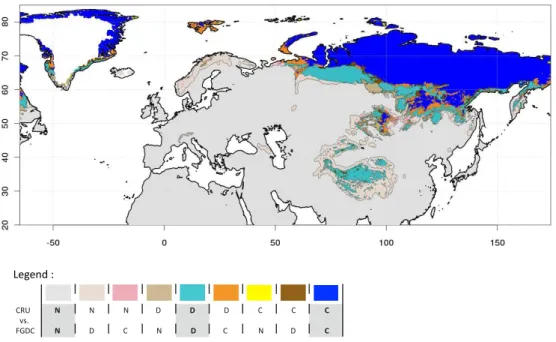
grouped into one circum-artic permafrost map by the International Permafrost Asso-ciation (IPA) and the Frozen Ground Data Center (FGDC) (Heginbottom et al., 1993; Brown et al., 1997). Most of permafrost data are observations between 1960 and 1980. LGM data correspond to a recent map of permafrost extent maximum in Europe and Asia around 21 ky BP, based on geological observations as described in

Vanden-10

berghe et al. (2008) and (2010). Consequently, our region of interest corresponds to the Eurasian continent with the Greenland ice-sheet approximately from 65° E to 175° W and from 20° N to 85° N (see Fig. 1). We consider the Greenland ice-sheet in order to calibrate our statistical model with the widest possible present temperature range for a downscaling on the LGM climate. These two maps have been drawn in

15

a similar way and both datasets describe the spatial distribution of two main types of permafrost (French, 2007):

– continuous permafrost is a permanently frozen ground which covers more than 80% of the sub-soil.

– discontinuous permafrost covers between 30% and 80% of sub-soil. The

perma-20

(7)

TCD

4, 2233–2275, 2010

Title Page

Tables Figures

◭ ◮

Back Close

Full Screen / Esc

Discussion

P

a

per

|

Dis

cussion

P

a

per

|

Discussion

P

a

per

|

Discussio

n

P

a

per

|

3 Downscaling with a Generalized Additive Model (GAM)

A GAM cannot directly simulate a discrete variable such as permafrost. We thus decide to downscale the temperatures from different CMs with the same approach as Vrac et al. (2007b) and Martin et al. (2010a). Then, we deduce permafrost from the local temperatures using a simple relationship between permafrost and temperature. This

5

methodology is illustrated in Fig. 2 (left half).

3.1 Temperature data and permafrost relationship

To calibrate our GAM, we need observations. The local-scale data used for the down-scaling scheme are the gridded temperature climatology from the Climate Research Unit (CRU) database (New et al., 2002). For each grid-point the dataset counts twelve

10

monthly means from 1961 to 1990 at a regular spatial resolution of 10′ (i.e. 1/6 de-gree in longitude and latitude) corresponding to our downscaling resolution. Although this period corresponds to the permafrost observations, permafrost is probably not in equilibrium with present climate and more with preindustrial simulations from CMs. In the following, we will consider the climate as the steady-state and assume that the

15

permafrost is in equilibrium with it.

In order to obtain the permafrost limits from the downscaled temperatures, we derive a local permafrost index according to the hypothesis that permafrost depends solely on temperature. Several relationships exist in literature (Nechaev, 1981; Huijzer and Isarin, 1997), we use the following conditions from Renssen and Vandenberghe (2003)

20

(explicitly described in Vandenberghe et al., 2004), which we will assign the name “RV”:

– continuous permafrost:

annual mean temperature6−8 °C and

coldest month mean temperature6−_{20 °C.}

– discontinuous permafrost:

25

(8)

TCD

4, 2233–2275, 2010

Title Page

Tables Figures

◭ ◮

Back Close

Full Screen / Esc

Discussion

P

a

per

|

Dis

cussion

P

a

per

|

Discussion

P

a

per

|

Discussio

n

P

a

per

|

To check the consistency of this assumption of permafrost being only related to perature, Fig. 1 compares the permafrost distribution obtained by applying these tem-perature conditions on CRU climatology, with the permafrost index from IPA/FGDC. The similarities between both representations are obvious and show a consistent rela-tionship between the two variables. Some di_fferences exist in high mountains regions

5

on the type or presence of permafrost. Indeed, even if this isotherm combination is calibrated on the present climate, the temperature is not the only criteria to model per-mafrost: for example, snow cover, soil and vegetation types have key roles for moun-tain permafrost (Guglielmin et al., 2003; French, 2007). Nevertheless to a first order, deriving permafrost from temperature is a reasonable approximation for present-day

10

conditions.

3.2 Generalized Additive Model

We first use a statistical model applied by Vrac et al. (2007a) to downscale climato-logical variables and based on the Generalized Additive Models (GAMs) as precisely studied in this context by Martin et al. (2010a). GAM models statistical relationships

15

between local-scale observations (called predictand) and large-scale variables (called predictors), generally from fields of CMs. The large-scale predictors will be described in Sect. 3.2.1. More precisely, this kind of statistical model models the expectation of the explained variableY (the predictand, surface temperature in our case) by a sum of nonlinear regressions with cubic splines (f_k), conditionally on the predictorsX_k(Hastie

20

and Tibshirani, 1990):

E(Y_i|X_k,k₌₁_...n) = n

X

k=1

f_k(X_{i ,k}) + ǫ, (1)

whereǫis the residual or error,nis the number of predictors andi is the grid-cell. To use GAM, we need to precise the distribution family of the explained variable. For simplicity, we assume that temperature have a gaussian distribution which implies

(9)

TCD

4, 2233–2275, 2010

Title Page

Tables Figures

◭ ◮

Back Close

Full Screen / Esc

Discussion

P

a

per

|

Dis

cussion

P

a

per

|

Discussion

P

a

per

|

Discussio

n

P

a

per

|

a zero-mean gaussian errorǫ (Hastie and Tibshirani, 1990). Then, any SDM needs a calibration/projection procedure. The calibration is the fitting process of the splines on present climate. Afterward, we project on a different climate to compute a temper-ature climatology in each grid-point of our region. Initially, the calibration step takes into account the 12 months of the climatology (annual calibration). To be evaluated in

5

fair conditions, the statistical model requires independent data between the calibration and projection steps. Using climatology data does not satisfy this condition on present climate with an annual calibration. As a workaround, we adapt a “cross-validation” pro-cedure which consists in a calibration on 11 months and a projection on the remaining month. With a rotation of this month, we are able to project a local-scale climatology

10

for any month.

In this paper, we only use GAM as a “tool” and we do not directly discuss the behavior of the statistical model; for more details we refer the reader to Vrac et al. (2007a); Martin et al. (2010a,b) and to the “mgcv” R package reference manual (downloadable at http://cran.r-project.org/).

15

3.2.1 Explanatory variables (predictors)

Previous studies from Vrac et al. (2007a) and Martin et al. (2010a) lead us to select four informative predictors for temperature downscaling, fully described in their stud-ies. Note that we only downscale on the continents because CRU data are only defined on land grid-points. Most of the predictors are computed from a representative set of

20

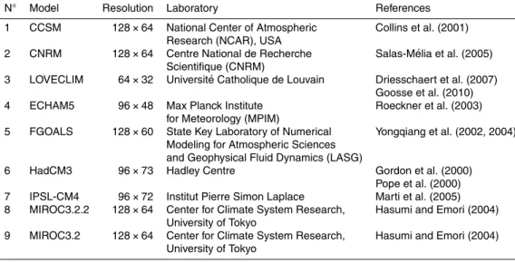
coupled ocean-atmosphere simulations provided by the Paleoclimate Modeling Inter-comparison Project (PMIP2) using state-of-the-art CMs. We choose to work with nine of them listed in Table 1. The explanatory variables may be divided into two groups: the “physical” predictors and the “geographical” ones. The “physical” predictors are directly extracted from CMs outputs and depend on climate dynamics. The “geographical”

pre-25

(10)

TCD

4, 2233–2275, 2010

Title Page

Tables Figures

◭ ◮

Back Close

Full Screen / Esc

Discussion

P

a

per

|

Dis

cussion

P

a

per

|

Discussion

P

a

per

|

Discussio

n

P

a

per

|

Here only one “physical” predictor is used and corresponds to the surface air tem-perature (SAT). This variable is extracted from present and LGM simulations from CMs bilinearly interpolated at 10′ resolution. If the interpolation may have an impact on our downscaling, we do not discuss this point in this study. A first test (not shown) reveals a cold bias from the nine CMs. Indeed, the present (preindustrial) simulations from

5

PMIP2 do not correspond to the 1961–1990 period of CRU data particularly in terms of CO2concentration. To account for this effect and to have a more relevant calibration

we correct CMs temperatures by adding for each CM the mean di_fference between itself and CRU climatology before calibration. For LGM period, we do not assume any temporal shift of the simulations. Consequently, we do not apply a similar correction on

10

LGM temperatures and we consider LGM permafrost in equilibrium with LGM climate. The “geographical” predictors are the topography and two continentality indices. The surface elevation from CMs depends on the resolution and does not account for small orographic structures. To take into account the e_ffect of local topography, we use the high-resolution gridded dataset, ETOPO21, from the National Geophysical Data

Cen-15

ter (NGDC) which gathers several topographic and bathymetric sources from satellite data and relief models (Amante and Eakins, 2008). We build the LGM topography from ETOPO2 adding in each grid-point a value corresponding to the difference between LGM and present orography. This difference is calculated using the ice-sheet model GRISLI (Peyaud et al., 2007) to account for the ice-sheet elevation and subsidence,

20

and the sea-level changes. The first continentality index is the “diffusive” continentality (DCO). DCO is between 0 and 100% and can be assimilated to the shortest distance to the ocean, 0 being at the ocean edge and 100 being very remote from any ocean. The physical interpretation is the effect of coastal atmospheric circulation on temperature. DCO does not depend on time and is only affected by sea-level change (or land-sea

25

distribution). The second continentality index is the “advective” continentality (ACO).

1

(11)

TCD

4, 2233–2275, 2010

Title Page

Tables Figures

◭ ◮

Back Close

Full Screen / Esc

Discussion

P

a

per

|

Dis

cussion

P

a

per

|

Discussion

P

a

per

|

Discussio

n

P

a

per

|

ACO is somewhat similar to DCO albeit being modulated by the large-scale wind in-tensities and directions from CMs and represents an index of the continentalization of air masses. It is based on the hypothesis that an air parcel becomes progressively continental as it travels over land. Hence ACO depends on the changes of land-sea distribution and on wind fields coming from the CMs simulations.

5

3.2.2 GAM results on present climate

In this section, GAM is applied to the nine CMs from the PMIP2 database. In order to make a visual comparison with data and to highlight the influence of downscaling on permafrost modelling, we compare permafrost distributions deduced from interpolated and from downscaled temperatures for each CM. We will assign the name of

“GAM-10

RV” for the procedure which consists in applying the RV conditions on temperatures downscaled by GAM. In the following, we only discuss the results from two representa-tive models: on the one side ECHAM5 (“ECHAM”) is heavily influenced by downscaling and shows the best results on CTRL period. One the other side, IPSL-CM4 (“IPSL”) is the coldest CM leading to good downscaling results on LGM. Note that we also mask

15

the ice-sheets (Greenland and Fennoscandia for LGM) as the presence of permafrost under an ice-sheet is not obvious and is currently debated. For example, Cutler et al. (2000) showed that a subglacial permafrost occurred during LGM with a numerical flow-line model. Harris and Murton (2005) argued, on the contrary, that variable de-grees of interaction exist between permafrost and glacial phenomena depending on

20

proximity to ice masses, exchanges of energy and transfers of water and ice. They concluded that the presence of ice-cover fundamentally alters the geothermal regime within a permafrost region. Moreover, since our estimate is based on surface temper-ature there is no reason why the permafrost under the ice-sheet shall be mainly driven by surface temperature, above the ice-sheet.

(12)

TCD

4, 2233–2275, 2010

Title Page

Tables Figures

◭ ◮

Back Close

Full Screen / Esc

Discussion

P

a

per

|

Dis

cussion

P

a

per

|

Discussion

P

a

per

|

Discussio

n

P

a

per

|

Figures 3a and 4a compare permafrost extents from interpolated temperatures (re-spectively for ECHAM and IPSL) when applying the RV conditions to derive per-mafrost, with the permafrost distribution from IPA/FGDC. The two maps reveal a lot of differences between CMs and data at high latitudes and in mountain regions, especially in Himalayas for ECHAM and in eastern Siberia for IPSL. Even if IPSL has a higher

5

resolution (Table 1), improving the representation of regional topographic structures, it does not contain enough local information to represent the permafrost distribution from IPA/FGDC data. Applying our GAM-RV approach, we obtain the corresponding Figs. 3b and 4b. Downscaling shows better permafrost distributions, particularly for discontinuous permafrost at high latitudes. For both CMs, some differences with data

10

disappear and the major contribution of local topography clearly appears for ECHAM with the onset of colder temperatures over the Siberian mounts or Himalayas. However, the information provided by inferred local temperatures cannot reduce the differences on the Scandinavian peninsula and around Himalayas or in eastern Siberia for IPSL.

To quantitatively assess the effect of our downscaling on permafrost representation,

15

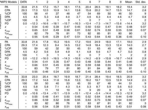
we measure the agreement between CMs and data for CTRL period with different nu-merical indices whose results are listed in Table 2. The first necessary informations are the total permafrost area (PA) and the permafrost area difference with data (PD). Without GAM-RV downscaling, CMs underestimate the permafrost area. Contrary to our expectations, the PA and consequently the PD decrease with GAM-RV

downscal-20

ing of about 106km2 for both CMs in comparison with interpolated fields. In order to distinguish between continuous and discontinuous permafrost, we detail their respec-tive areas (CPA and DPA). The decrease of permafrost area is mainly explained by a decrease of the continuous permafrost area of about 0.8×106km2 for both CMs. The DPA slightly increases for ECHAM (+0.2×106km2) and decreases (−0.3×106km2) for

25

(13)

TCD

4, 2233–2275, 2010

Title Page

Tables Figures

◭ ◮

Back Close

Full Screen / Esc

Discussion

P

a

per

|

Dis

cussion

P

a

per

|

Discussion

P

a

per

|

Discussio

n

P

a

per

|

cases, it increases %DP from 16 to 31% for ECHAM, while it decreases for IPSL. The responses of these two climate models show the limits of the GAM method. On aver-age GAM-RV essentially enhances the discontinuous permafrost distribution (+4%DP), more reducing the continuous permafrost area (−0.9×106km2) than increasing the discontinuous permafrost extent (+0.1×106km2). Moreover, Fig. 5a shows the

box-5

and-whisker plots for all interpolated and downscaled CMs. We confirm the decrease of permafrost area for most of downscaled CMs by GAM-RV with a mean relative dif-ference with data of−25.2% against−20.4% for the interpolated CMs. The plots also reveal a weaker inter-variability between CMs with downscaling. Indeed, in Table 2 our GAM-RV reduces the standard deviation for all area indices (for example, from 0.7 to

10

0.5 for PA).

These area indices provide numerical information on the permafrost extents but do not quantify the statistical relevance of agreement between CMs and data. To judge if we do not obtain these results “by chance”, we use the kappa coe_fficient (κ). This index between 0 and 1 measures the intensity or quality of the agreement based on

15

a simple counting of grid-points in a confusion/matching matrix (Cohen, 1960; Fleiss et al., 1969). The following example details the calculation of theκcoe_fficient (Eq. 4):

Model

Total

C D N

Data

C n₁_,₁ n₁_,₂ n₁_,₃ n₁_,.

D n₂_,₁ n₂_,₂ n₂_,₃ n₂_,.

N n₃_,₁ n₃_,₂ n₃_,₃ n₃_,.

Total n_.,₁ n_.,₂ n_.,₃ n

P_obs ₌ 1 n

3

X

i=1

(14)

TCD

4, 2233–2275, 2010

Title Page

Tables Figures

◭ ◮

Back Close

Full Screen / Esc

Discussion

P

a

per

|

Dis

cussion

P

a

per

|

Discussion

P

a

per

|

Discussio

n

P

a

per

|

P_chance ₌ 1

n2 3

X

i=1

n_{i ,.} ×n_.,i, (3)

κ ₌ Pobs −Pchance

1 − P_chance , (4)

where “C”, “D” and “N” corresponds to our three categories “Continuous”, “Discontinu-ous” and “No” permafrost,n_{i ,j} are the cell counts with the classification totalsn_{i .} and

n_.j,nis the number of grid-cells,P_obs (Eq. 2) is the proportion of observed agreement

5

andP_chance(Eq. 3) is the proportion of random agreement or expected by chance with

independent samples.

Without downscaling, ECHAM obtains a κ of 0.64 and 0.68 for IPSL. To gauge the strength of agreement without an arbitrary scale, we use the kappa maximum (κ_max). Based on the same counting as theκ, it estimates the best possible agreement (the

10

maximum attainable κ). We adjust the cell counts (n_{i ,j}) maximizing the agreement (cellsn_{i ,j}₌_i) keeping the same classification totals of each category for CMs and data (n_{i .}and n_.j): this allows a more appropriate scaling ofκ (Sim and Wright, 2005). The difference betweenκand 1 indicates the total unachieved agreement. Accordingly, the difference between κ and κ_max indicates the unachieved agreement beyond chance

15

and the difference betweenκ_maxand 1 shows the effect on agreement of pre-existing factors that tend to produce unequal classification totals, such as nonlinearities or dif-ferent sensitivities of CMs. Moreover to provide useful information to interpret the mag-nitude of κ coefficient, we add the percentage of κ_max reached by κ (%κ_max). Thus, without downscaling ECHAM (IPSL) reaches 72% (74%) of a maximum agreement

20

beyond chance of 0.88 (0.91). With GAM-RV, the %κ_max increases for both CMs due to an increase of κ and a lower κ_max. Calculation of the κ coefficient implies intrin-sic biases (Cicchetti and Feinstein, 1990). The adjusted kappa (κ_adj, also called the prevalence-adjusted bias-adjusted kappa – PABAK) is also based on the same count-ing as the κ with adjusted cell counts minimizing those intrinsic biases. It gives an

25

(15)

TCD

4, 2233–2275, 2010

Title Page

Tables Figures

◭ ◮

Back Close

Full Screen / Esc

Discussion

P

a

per

|

Dis

cussion

P

a

per

|

Discussion

P

a

per

|

Discussio

n

P

a

per

|

κ_adj is close toκ, then the bias is weak (Sim and Wright, 2005). κ_adj is necessary to interpret in an appropriate manner the statistical significance ofκ coefficient. Here, all studied CMs obtain a κ_adj close to their κ. Consequently, the results obtained by GAM-RV are statistically relevant, in better agreement with data and not by chance.

Despite heterogeneous contributions from GAM on permafrost distribution, this

5

method is informative for temperature downscaling on CTRL period. All CMs obtained a percentage of explained variance between 97 and 100%. GAM brings downscaled CMs closer to the CRU climatology improving the temperature distribution (Vrac et al., 2007a; Martin et al., 2010a). We confirm that the RV relationship does not provide enough information for local permafrost distribution and leads to a close dependence

10

between temperature and permafrost. The permafrost distribution from CMs is strongly driven by the latitudinal gradient of SAT, leading to a disagreement with data. Further-more, applying the RV conditions on CRU temperatures leads to a PA of 10.4×106km2. Based on the hypothesis that CRU and CTRL permafrost data have no uncertainties, the RV relationship induces an error of−26.0% compared to permafrost data (Fig. 5a).

15

Consequently, GAM-RV includes this error and does not improve the permafrost distri-bution beyond the CRU permafrost distridistri-bution.

4 An alternative approach: the Multinomial Logistic Regression

Using temperature downscaling to reconstruct permafrost limits requires conditions to go from continuous to discrete values. As shown in Sects. 3.1 and 3.2.2, the RV

20

relationship is only based on the contribution of temperature for permafrost distribution. A study at a local-scale needs more informations. Here, we propose to enlarge the spectrum of relationships between permafrost and several factors.

To link a categorical variable, such as permafrost, with several variables, we model the probability of occurrence of permafrost. This probability can take continuous

val-25

(16)

TCD

4, 2233–2275, 2010

Title Page

Tables Figures

◭ ◮

Back Close

Full Screen / Esc

Discussion

P

a

per

|

Dis

cussion

P

a

per

|

Discussion

P

a

per

|

Discussio

n

P

a

per

|

instance, Calef et al. (2005) build a hierarchical logistic regression model (three bi-nary logistic regression steps) to predict the potential equilibrium distribution of four major vegetation types. More classically, Fealy and Sweeney (2007) use the logistic regression as SDM to estimate the probabilities of wet and dry days occurrences. Here, we use the logistic regression in its multinomial form (Multinomial Logistic Regression

5

– MLR – Hilbe, 2009; Hosmer and Lemeshow, 2000) to simulate the occurrence prob-ability of a permafrost index, as illustrated in Fig. 2 (right half). MLR is used as a SDM to estimate the occurrence probabilities of the explained variable (Y, permafrost in our case) for each category or classj, taking into account numerical or categorical predictors (X_k):

10

log

_P₍_Y

i = j)

1 − P(Y_i ₌ j)

= n

X

k=1

β_k X_{i ,k}, (5)

whereP(Y_i₌j) is the probability of thej-th permafrost category withPm

j=1P(Yi=j)=1

(considering mcaterogies), β_k are the regression coefficients for the j-th permafrost category,nis the number of predictors andi is the grid-cell.

The method is based on the use of a Generalized Linear Model (GLM –

McCul-15

lagh and Nelder, 1989). GLM generalizes linear regression using a link function be-tween predictand and predictors unifying various statistical regression models, includ-ing linear regression, Poisson regression and logistic regression. For more details see Yee and Wild (1996) and the “VGAM” R package reference manual (downloadable at http://cran.r-project.org/).

20

Local-scale data used for the calibration step are directly the local-scale observed permafrost indices (IPA/FGDC). In order to compare MLR and GAM-RV we use the same predictors for both methods. As said in Sect. 3.1, the topography, SAT and continentality indices were chosen for temperature downscaling. Although SAT and the topography are clearly necessary for permafrost representation, a study on the

25

(17)

TCD

4, 2233–2275, 2010

Title Page

Tables Figures

◭ ◮

Back Close

Full Screen / Esc

Discussion

P

a

per

|

Dis

cussion

P

a

per

|

Discussion

P

a

per

|

Discussio

n

P

a

per

|

In GAM-RV we had to set the relationship between permafrost and downscaled temperatures. Here, MLR builds a new relationship between permafrost and the se-lected predictors which can be compared to the previous isotherms combinations from Renssen and Vandenberghe (2003). Figure 6 shows the probabilities to obtain each category of permafrost in each approach. On the panels 6a–c, we apply the RV

con-5

ditions on CRU temperatures. On the panels 6d–f, we model by MLR the relationship between permafrost from IPA/FGDC and two predictors: the annual mean tempera-ture and the coldest month mean temperatempera-ture from CRU. Thus, each graph on the left is directly comparable to the corresponding one on the right (Fig. 6). Conditions from Renssen and Vandenberghe (2003) clearly appears with probabilities of 0 or 1

10

depending on the isotherms described in Sect. 3.1. With MLR, visible similarities with the relationships used in GAM-RV demonstrates the consistency of the method. How-ever, the probabilities can take continuous values between 0 and 1 and allows us to obtain for each grid-point three complementary probabilities for the continuous, discon-tinuous and no permafrost categories. For example, contrary to GAM-RV, condiscon-tinuous

15

permafrost with a probability of 1 requires a annual mean temperature below−8 °C, but extends to coldest month mean temperatures above−20 °C. In MLR, the modeled re-lationship also varies according to the selected predictors and the studied CM. Bypass-ing temperature downscalBypass-ing allows computBypass-ing a more complex relationship between predictors and permafrost. Moreover, MLR could take into account other permafrost

20

categories (e.g. sporadic or isolated permafrost; French, 2007).

4.1 Comparison GAM vs. MLR on present climate

To confront MLR with GAM, Figs. 3c and 4c compare the permafrost indices down-scaled by MLR (respectively for ECHAM and IPSL) with the permafrost distribution from IPA/FGDC data. The permafrost indices downscaled by MLR correspond in each

grid-25

(18)

TCD

4, 2233–2275, 2010

Title Page

Tables Figures

◭ ◮

Back Close

Full Screen / Esc

Discussion

P

a

per

|

Dis

cussion

P

a

per

|

Discussion

P

a

per

|

Discussio

n

P

a

per

|

in Himalayas and Tibetan plateau and in other areas with mountain permafrost (Scan-dinavian mounts, Alps, Siberian mounts). For both CMs, most of the differences per-sisting with the GAM downscaling disappear with MLR, as in eastern Siberia for IPSL. In Table 2, the MLR downscaling improves the permafrost area for ECHAM (+2.7×

106km2) and IPSL (+1.2×106km2), increasing the CPA and the DPA in both cases,

5

in comparison with interpolated CMs. The percentages of continuous or discontinuous areas in agreement with data also increase to values close to 90% for %CP and 53% for %DP. The box-and-whisker plot for MLR downscaling (Fig. 5a) clearly shows im-provements for all CMs with a mean relative difference with data of−10.6%, compared with GAM-RV (−25.2%).

10

Moreover, the permafrost distribution is very similar between ECHAM and IPSL. The same patterns can also be observed on the maps of the different CMs (not shown) especially for continuous permafrost. Figure 5a clearly shows that MLR reduces the inter-variability between CMs, more than with GAM-RV. Indeed, MLR has a weaker standard deviation whatever the index (for example, 0.2×106km2 for PA). This

al-15

ternative method brings all climate models closer to the permafrost distribution from IPA/FGDC data.

In terms ofκ statistics, MLR systematically improves the statistical agreement from 0.64 to 0.79 for ECHAM and from 0.68 to 0.78 for IPSL. No significant changes appears for theκ_max. So, the higher %κ_maxdirectly reflects a better agreement with data. Note

20

that the standard deviation is also reduced forκ indices: the quality of the agreement is equal for all CMs. MLR provides more confidence on the fact that our results are not obtained “by chance”. Moreover, all CMs have aκ_adj closer to κ than with GAM-RV: the intrinsic biases are slightly weaker with MLR.

Nevertheless, this method also reveals some inconsistencies. Incorrect transitions

25

(19)

TCD

4, 2233–2275, 2010

Title Page

Tables Figures

◭ ◮

Back Close

Full Screen / Esc

Discussion

P

a

per

|

Dis

cussion

P

a

per

|

Discussion

P

a

per

|

Discussio

n

P

a

per

|

type and snow cover could bring more consistent physics to build a high-resolution per-mafrost.

In conclusion, bypassing temperature downscaling provides an adapted relationship between permafrost and predictors for each CM, leading to a more precise spatial representation of permafrost and a better agreement with observed data, at CTRL

5

period.

Our results are the byproduct of several factors such as: the ability of CMs to cor-rectly represent temperature, the relationship between permafrost and chosen vari-ables, etc. It is thus difficult to independently quantify the error of each factor in the final result. Such a sensitivity analysis is beyond the scope of our paper and will be the

10

subject of further studies.

5 Application to LGM permafrost

In a climate change context it is interesting to test the ability of our statistical models to represent past climates when they have been calibrated on present climate. In terms of temperatures and precipitation Martin et al. (2010b) obtain remarkable results from the

15

EMIC CLIMBER (Ganopolski et al., 2001; Petoukhov et al., 2000) in comparison with GCMs outputs for the Last Glacial Maximum (LGM) climate and conclude to a great potential of GAM for applications in paleoclimatology (Vrac et al., 2007a; Martin et al., 2010b).

Can we thus export our statistical models at a different past climate, as the LGM,

20

in terms of permafrost distribution? To answer this question, we apply our two SDMs on LGM outputs from the PMIP2 CMs. For this time period, the permafrost distribution used to compare with CMs is from Vandenberghe et al. (2010).

Figures 7a and 8a compare the permafrost distribution from interpolated CMs (with the RV conditions) with the permafrost distribution from data. Without downscaling,

25

(20)

TCD

4, 2233–2275, 2010

Title Page

Tables Figures

◭ ◮

Back Close

Full Screen / Esc

Discussion

P

a

per

|

Dis

cussion

P

a

per

|

Discussion

P

a

per

|

Discussio

n

P

a

per

|

ice-sheet contours. Moreover, its coarse orography is not enough to represent moun-tain permafrost in Himalayas. IPSL is colder and has a higher resolution, providing a more representative permafrost distribution around the ice-sheet and the Tibetan plateau. Figures 7b and 8b compare in the same way the permafrost distribution from GAM-RV with the permafrost distribution from Vandenberghe et al. (2010). The

5

contribution of the local-scale topography appears particularly with the onset of moun-tain permafrost in Himalayas for ECHAM as for present climate. For IPSL, GAM slightly warms temperatures, leading to permafrost limits at higher latitudes. Permafrost down-scaled with MLR is compared with data in Figs. 7c and 8c. For the ECHAM model, the local-scale topography also brings up the Himalayas and Tibetan plateau, but the

tran-10

sitions from continuous to no permafrost are more numerous (blue to pink colors on Fig. 7c). MLR applied to IPSL shows a weaker effect of the local topography but the permafrost limits reach lower latitudes than interpolated CMs or GAM-RV, especially the southern regions of the Fennoscandian ice-sheet.

We give in Table 3 the numerical indices for LGM period. Quantitatively,

GAM-15

RV does not systematically improve the permafrost area: +1.4 for ECHAM and

−1.6×106km2for IPSL with respect to interpolated fields. Even if GAM-RV degrades the permafrost distribution for IPSL, it remains the best representation with the highest %CP (63%) and %DP (7%) for this method. With MLR downscaling, the results are improved for both CMs at the same order than CTRL period (about+1.5×106km2

be-20

tween interpolated and downscaled CMs). Moreover, we obtain higher %CP and %DP than GAM-RV for all CMs. Nevertheless, with both SDMs the surface differences with data are more important than CTRL period. The CMs underestimates the continuous permafrost area and no or less discontinuous permafrost is simulated in right location (%DP ranges between 0 and 20%). No significant decrease appears in terms of

inter-25

(21)

TCD

4, 2233–2275, 2010

Title Page

Tables Figures

◭ ◮

Back Close

Full Screen / Esc

Discussion

P

a

per

|

Dis

cussion

P

a

per

|

Discussion

P

a

per

|

Discussio

n

P

a

per

|

and GAM-RV simulations are not significantly different; same results appears for their means with a Student’s test. This shows that the permafrost distribution at the LGM is strongly driven by the large-scale temperature from CMs. Our SDMs cannot correct the large gap between interpolated CMs and permafrost data at LGM (Fig. 5b). With a simulated LGM climate closer to data, downscaling could have more impact: it is the

5

case of the IPSL model with a contribution of downscaling in the same order that CTRL period (Tables 2 and 3). Consequently, we cannot base our interpretation of the LGM results on CTRL results.

The larger differences with data than at CTRL period imply a lower κ coefficient (Table 3). With GAM-RV no changes appear for ECHAM except for theκ_adj showing

10

larger biases in calculation ofκ. For IPSL theκcoe_fficient decreases from 0.63 to 0.58. GAM-RV does not improve the statistical agreement, reflecting the weak potential of CMs to correctly represent permafrost limits for the LGM period. MLR obtains the best results improving slightly the agreement with data for all CMs.

We can summarize with some remarks:

15

i. the contribution of GAM is not su_fficient to reduce the gap between CMs and data in reproducing local-scale permafrost. MLR produces a more realistic permafrost distribution reaching latitudes similar to those from data and improving the agree-ment with it. Nevertheless, our SDMs do not reduce the inter-variability between CMs at LGM.

20

ii. our SDMs includes the strong contribution of surface temperature and topography. Nevertheless as for CTRL period, the predictors ACO and DCO are not informa-tive for permafrost. So common differences appear between the two periods. De-spite consistent patterns, the permafrost distribution is still strongly driven by the latitudinal gradient of SAT for GAM-RV and incorrect transitions from continuous

25

to no permafrost appears with MLR.

(22)

TCD

4, 2233–2275, 2010

Title Page

Tables Figures

◭ ◮

Back Close

Full Screen / Esc

Discussion

P

a

per

|

Dis

cussion

P

a

per

|

Discussion

P

a

per

|

Discussio

n

P

a

per

|

that the relationships between permafrost and chosen variables are stable with time, the nine climate models from PMIP2 cannot simulate a cold enough climate to represent the LGM period. They have a warm bias that cannot be completely corrected by one of the two tested SDMs calibrated on present climate.

iv. the di_fferences observed between downscaled CMs and data partly come from

5

the relationship between permafrost and the other variables. The RV conditions are based on present observations. The relationship between permafrost and predictors from MLR is also calibrated on the CTRL period. Do these relationships be the same during the LGM period? The continuous or discontinuous permafrost extents may not be defined by the same isotherms seen in Sect. 3.1; in the case

10

of MLR, the influence of different predictors may change in another climate.

v. finally, LGM permafrost data are best currently available and based on geological observations of the maximum permafrost extent and correspond to the coldest time period around LGM (21 kyr BP). The LGM time period is defined with the maximum extent of the ice-sheets which is probably not directly related to

tem-15

perature minimum. In the high-resolution record from the North Greenland Ice Core Project (NGRIP, Andersen et al., 2004), the last temperature minimum ap-pears at about 34 kyr BP. A lag may exist between the LGM data and the LGM cli-mate simulated by clicli-mate models. Therefore, LGM permafrost data are likely to be overestimated. The differences between downscaled permafrost from PMIP2

20

models and LGM permafrost extent from Vandenberghe et al. (2010) should be taken as a gross estimate.

6 Conclusions

We described two statistical downscaling methods (SDMs) for permafrost studies. In order to obtain high-resolution permafrost spatial distribution, we first applied these

25

(23)

TCD

4, 2233–2275, 2010

Title Page

Tables Figures

◭ ◮

Back Close

Full Screen / Esc

Discussion

P

a

per

|

Dis

cussion

P

a

per

|

Discussion

P

a

per

|

Discussio

n

P

a

per

|

Generalized Additive Model (GAM) is suitable for representing the temperature behav-ior at a local-scale (Vrac et al., 2007b). According to Martin et al. (2010a) results, choosing a GAM leads to a relevant physical model for the small scales with simple statistical relationships that are easily interpretable. Applying the conditions defined by Renssen and Vandenberghe (2003) on downscaled temperatures improves the

spa-5

tial distribution of discontinuous permafrost but underestimates the permafrost area. This GAM-RV method reaches some limits with a permafrost strongly driven by the latitudinal gradient of temperatures. Indeed a simple combination of isotherms is not sufficient to describe the permafrost distribution at a local-scale. The approach by Multinomial Logistic Regression (MLR) is more adapted for this application. The

mod-10

eled relationship, as a function of several variables, provides a better representation of continuous permafrost and mountain permafrost (especially discontinuous permafrost) and reduces the inter-variability between all climate models from PMIP2 database with a larger statistical relevance. The results from MLR confirm that a study at a local-scale needs more physics about permafrost.

15

Applying our SDMs on a different climate, the Last Glacial Maximum (LGM), leads to permafrost distribution in better agreement with data, especially for MLR downscaling. Nevertheless downscaling of LGM permafrost extent faces difficulties with larger diff er-ences than CTRL period. None of the studied climate models can represent a LGM permafrost extent comparable to data, whatever the method used. The inter-variability

20

between climate models strongly depends on large-scale temperature that cannot be completely corrected by our SDMs. The differences with data reduce the contribution of downscaling and have di_fferent sources: (i) an assumed stationarity of the RV con-ditions for GAM and the modeled relationship for MLR; (ii) an initial bias from climate models which cannot simulate a proper LGM climate; (iii) a complex permafrost

dy-25

(24)

TCD

4, 2233–2275, 2010

Title Page

Tables Figures

◭ ◮

Back Close

Full Screen / Esc

Discussion

P

a

per

|

Dis

cussion

P

a

per

|

Discussion

P

a

per

|

Discussio

n

P

a

per

|

To complement this study, some points would deserve to be deepened to improve our results. Permafrost is an heterogeneous variable with few observations. Climate models temperature, used to derive permafrost distribution, is a global and continu-ous variable. Therefore, we need local-scale predictors that will add local variability to climate signal. Our SDMs use local-scale topography but other variables used in

per-5

mafrost dynamic models, as vegetation or soil properties (Marchenko et al., 2008), are required to have a representative physics of permafrost processes and a better distri-bution. The potential of the MLR approach lies in the control of the physics included in the predictors. In this study we used the same predictors for both SDMs. It is obvious that they can and should be changed in the MLR method to represent more accurately

10

the permafrost distribution. This ongoing work will take into account large-scale fields of snow cover and thickness and soil temperature. We can also imagine to build new “geographical” predictors such as exposure to the sun depending on the orientation of the topography slope (Brown, 1969). The balancing and choice of “geographical” and “physical” predictors is crucial to maintain good local representation and a consistent

15

and robust physical model applicable to different climates. To reconcile models and data, it would also be interesting to downscale permafrost at colder periods simulated by climate models, such as Heinrich events (Kageyama et al., 2005). We would be able to determine the needed temperatures to obtain the best permafrost limits according to the data from Vandenberghe et al. (2010).

20

Acknowledgements. We thank J. Vandenberghe (Centre for Geo-ecological Research, Nether-lands) for providing permafrost data for the Last Glacial Maximum period, C. Dumas for deriv-ing LGM topography from GRISLI data. G. Levavasseur is supported by UVSQ, D. Roche by INSU/CNRS.

(25)

TCD

4, 2233–2275, 2010

Title Page

Tables Figures

◭ ◮

Back Close

Full Screen / Esc

Discussion

P

a

per

|

Dis

cussion

P

a

per

|

Discussion

P

a

per

|

Discussio

n

P

a

per

|

The publication of this article is financed by CNRS-INSU.

References

Amante, C. and Eakins, B.: ETOPO1 – 1 arc-minute global relief model: procedures, data sources and analysis, National Geophysical Data Center, NESDIS, NOAA, US Department 5

of Commerce, Boulder, CO, 2008. 2242

Andersen, K., Azuma, N., Barnola, J.-M., Bigler, M., Biscaye, P., Caillon, N., Chappellaz, J., Clausen, B., Dahl-Jensen, D., Fischer, H., Fl ¨uckiger, J., Fritzsche, D., Fujii, Y., Goto-Azuma, K., Grønvold, K., Gundestrup, N., Hansson, M., Huber, C., Hvidberg, C., Johnsen, S., Jon-sell, U., Jouzel, J., Kipfstuhl, S., Landais, A., Leuenberger, M., Lorrain, R., Masson-Delmotte, 10

V., Miller, H., Motoyama, H., Narita, H., Popp, T., Raynaud, D., Rothlisberger, R., Ruth, U.,

Samyn, D., Schwander, J., Shoji, H., Siggard-Andersen, M.-L., Steffensen, J., Stocker, T.,

Sveinbj ¨ornsd ´ottir, A., Svensson, A., Takata, M., Tison, J.-L., Thorsteinsson, T., Watanabe, O., Wilhelms, F., and White, J.: High-resolution record of Northern Hemisphere climate ex-tending into the last interglacial period, Nature, 431, 147–151, doi:10.1038/nature02805, 15

2004. 2254

Anisimov, O. and Nelson, F.: Permafrost zonation and climate change in the northern hemi-sphere: results from transient general circulation models, Climatic Change, 35, 241–258, doi:10.1023/A:1005315409698, 1997. 2235

Anisimov, O., Shiklomanov, N., and Nelson, F.: Variability of seasonal thaw depth in per-20

mafrost regions: a stochastic modeling approach, Ecol. Model., 153, 217–227, doi:10.1016/ S0304-3800(02)00016-9, 2002. 2236

Beer, C.: The arctic carbon count, Nat. Geosci., 1, 569–570, doi:10.1038/ngeo292, 2008. 2235 Braconnot, P., Otto-Bliesner, B., Harrison, S., Joussaume, S., Peterchmitt, J.-Y., Abe-Ouchi, A.,

Crucifix, M., Driesschaert, E., Fichefet, Th., Hewitt, C. D., Kageyama, M., Kitoh, A., Laˆın ´e, A.,

(26)

TCD

4, 2233–2275, 2010

Title Page

Tables Figures

◭ ◮

Back Close

Full Screen / Esc

Discussion

P

a

per

|

Dis

cussion

P

a

per

|

Discussion

P

a

per

|

Discussio

n

P

a

per

|

Loutre, M.-F., Marti, O., Merkel, U., Ramstein, G., Valdes, P., Weber, S. L., Yu, Y., and Zhao, Y.: Results of PMIP2 coupled simulations of the MidHolocene and Last Glacial Maximum -Part 1: experiments and large-scale features, Clim. Past, 3, 261–277, doi:10.5194/cp-3-261-2007, 2007a. 2237

Braconnot, P., Otto-Bliesner, B., Harrison, S., Joussaume, S., Peterchmitt, J.-Y., Abe-Ouchi, 5

A., Crucifix, M., Driesschaert, E., Fichefet, Th., Hewitt, C. D., Kageyama, M., Kitoh, A., Loutre, M.-F., Marti, O., Merkel, U., Ramstein, G., Valdes, P., Weber, L., Yu, Y., and Zhao, Y.: Results of PMIP2 coupled simulations of the Mid-Holocene and Last Glacial Maximum – Part 2: feedbacks with emphasis on the location of the ITCZ and mid- and high latitudes heat budget, Clim. Past, 3, 279–296, doi:10.5194/cp-3-279-2007, 2007b. 2237

10

Brown, J., Ferrians, O., Heginbottom, J., and Melnikov, E.: Circum-Arctic map of permafrost and ground-ice conditions, Washington, DC: US Geological Survey in Cooperation with the Circum-Pacific Council for Energy and Mineral Resources, Circum-Pacific Map Series, CP-45, 1997. 2238

Brown, R.: Factors influencing discontinuous permafrost in Canada, in: The Periglacial Envi-15

ronment, Past and Present, edited by: P ´ew ´e, T., INQUA Seventh Congress, McGill-Queen’s University Press, Montreal, Canada, 11–53, 1969. 2256

Buishand, T., Shabalova, M., and Brandsma, T.: On the choice of the temporal aggregation level for statistical downscaling of precipitation, J. Climate, 17, 1816–1827, 2003. 2237 Calef, M., McGuire, A., Epstein, H., Rupp, T., and Shugart, H.: Analysis of vegetation distribu-20

tion in Interior Alaska and sensitivity to climate change using a logistic regression approach, J. Biogeogr., 32, 863–878, 2005. 2237, 2248

Christensen, J. and Kuhry, P.: High-resolution regional climate model validation and permafrost simulation for the East European Russian Arctic, J. Geophys. Res., 105, 29647–29658, doi: 10.1029/2000JD900379, 2000. 2236

25

Cicchetti, D. and Feinstein, A.: High agreement but low kappa – II. Resolving the paradoxes, J. Clin. Epidemiol., 43, 551–558, doi:10.1016/0895-4356(90)90159-M, 1990. 2246

Cohen, J.: A coe_fficient of agreement for nominal scales, Educational and Psychological

Mea-surement, 20, 37–46, doi:10.1177/001316446002000104, 1960. 2245

Collins, W., Bitz, C., Blackmon, M., Bonan, G., Bretherton, C., Carton, J., Chang, P., Doney, 30

(27)

TCD

4, 2233–2275, 2010

Title Page

Tables Figures

◭ ◮

Back Close

Full Screen / Esc

Discussion

P

a

per

|

Dis

cussion

P

a

per

|

Discussion

P

a

per

|

Discussio

n

P

a

per

|

Cutler, P., MacAyeal, D., Mickelson, D., Parizek, B., and Colgan, P.: A numerical investigation of ice-lobe-permafrost interaction around the southern Laurentide ice-sheet, J. Glaciol., 46, 311–325, 2000. 2243

Delisle, G.: Numerical simulation of permafrost growth and decay, J. Quaternary Sci., 13, 325– 333, doi:0.1002/(SICI)1099-1417(199807/08)13:4, 1998. 2235

5

Driesschaert, E., Fichefet, T., Goosse, H., Huybrechts, P., Janssens, I., Mouchet, A., Munhoven, G., Brovkin, V., and Weber, S. L.: Modeling the influence of Greenland ice sheet melting on the Atlantic meridional overturning circulation during the next millennia, Geophys. Res. Lett., 34, L10707, doi:10.1029/2007GL029516, 2007. 2265

Fealy, R. and Sweeney, J.: Statistical downscaling of precipitation for a selection of sites in 10

Ireland employing a generalised linear modelling approach, Int. J. Climatol., 27, 2083–2094, doi:10.1002/joc.1506, 2007. 2237, 2248

Fleiss, J., Cohen, J., and Everitt, B.: Large sample standard errors of kappa and weighted kappa, Psychol. Bull., 72, 323–327, doi:10.1037/h0028106, 1969. 2245

French, H.: The periglacial environment, 3rd Edition, Wiley, 2007. 2238, 2240, 2249 15

Ganopolski, A., Petoukhov, V., Rahmstorf, S., Brovkin, V., Claussen, M., Eliseev, A., and Ku-batzki, C.: CLIMBER-2: a climate system model of intermediate complexity – Part 2: model sensitivity, Clim. Dynam., 17, 735–751, doi:10.1007/s003820000144, 2001. 2251

Gladstone, R., Ross, I., Valdes, P., Abe-Ouchi, A., Braconnot, P., Brewer, S., Kageyama, M., Kitoh, A., Legrande, A., Marti, O., Ohgaito, R., Otto-Bliesner, B., Peltier, W., and Vettoretti, 20

G.: Mid-Holocene NAO: a PMIP2 model intercomparison, Geophys. Res. Lett., 32, L16707, doi:10.1029/2005GL023596, 2005. 2237

Goosse, H., Brovkin, V., Fichefet, T., Haarsma, R., Huybrechts, P., Jongma, J., Mouchet, A., Selten, F., Barriat, P.-Y., Campin, J.-M., Deleersnijder, E., Driesschaert, E., Goezler, H., Janssens, I., Loutre, M.-F., Maqueda, M., Opsteegh, T., Mathieu, P.-P., Munhoven, G., Pet-25

tersson, E., Renssen, H., Roche, D. M., Schaeffer, M., Tartinville, B., Timmermann, A., and

Weber, S.: Description of the earth system model of intermediate complexity LOVECLIM version 1.2, Geoscientific Model Development, 3, 309–390, doi:10.5194/gmdd-3-309-2010, 2010. 2265

Gordon, C., Cooper, C., Senior, C., Banks, H., Gregory, J., Johns, T., Mitchell, J., and Wood, 30