Navigation of Mobile Robots Using Potential Fields and Computational Intelligence Means

Navigation of Mobile Robots Using Potential

Fields and Computational Intelligence Means

Ján Vaš

č

ák

Centre for Intelligent Technologies, Department of Cybernetics and Artificial Intelligence, Faculty of Electrical Engineering and Informatics, Technical University in Košice

Letná 9, 042 00 Košice, Slovakia [email protected]

Abstract: A number of various approaches for robot navigation have been designed. However, practical realizations strike on some serious problems like imprecision of measured data, absence of complete knowledge about environment as well as computational complexity and resulting real-time bottlenecks. Each of proposed solutions has some of mentioned drawbacks. Therefore one of possible solutions seems to be in combining several means of computational intelligence. In this paper a combination of harmonic potential fields, neural networks and fuzzy controllers is presented. Also some simulation experiments are done and evaluated.

Keywords: harmonic potential fields, neural networks, fuzzy controller

1 Introduction

Theoretically the problem of finding the shortest or the safest path between two points in an environment with obstacles can be well defined and solved. Basically, there are three groups of approaches: heuristic, exact and grid algorithms (a good overview can be found in [4]). The first group is represented mainly by Bug algorithms, which are simple and suitable for environments with static obstacles. Exact algorithms, mainly visibility graphs and Voronoi diagrams, enable a mathematically correct way for finding the best solution. If there is no possible path (too restrictive obstacles) then they will be able to give a definite answer ‘no’. However, they require precise sensing of obstacles and are suitable above all only for static environments. Algorithms based on grid description are more convenient for practical use because the precision of sensing is limited.

to navigate a robot in a simple environment with only few obstacles and in the case of a more complicated area to switch to a more detailed grid description. There are also methods, which do not require having a complete map a priori. It can be constructed in steps, too [2]. It means they can be used also in dynamic environments. The only difference between static and dynamic environment is that in the second case the environment is changing during the movement of a robot, e.g. we consider vehicles or walkers.

However, also potential fields have some lacks, especially their computational complexity. Therefore, in this paper a structure combining potential fields with a neural network and fuzzy controller is proposed. The next section will describe basic principles of potential fields. Then the proposed structure will be described in detail and finally, some experiments and conclusions will be mentioned.

2 Potential

Fields

In general, there are two principal objects in each environment: goals (we will further consider only one goal) and obstacles. The goal should attract a robot to its position and obstacles should repulse it from them. Therefore we will speak about attractive Fr_G and repulsive Fr_O strengths, respectively. Considering a two-dimensional space X x Y the total strength Fr in a certain point will be given as a vector sum:

( , ) ( , ) ( , ).

i

G O

i

F x yr =Fr x y +

∑

A set of all strengths for all combinations of (x, y) creates a vector field Fr (see Fig. 2).

Potential U x y( , ) is numerically equal to the work done between this point and a point with a zero potential (x0, y0) along the path l, i.e.:

0 0 ( , )

( , )

( , ) . .

x y x y

U x y =

∫

Again, the depiction for all combinations of (x, y) creates a potential field U (see Fig. 1).

goal. There are lots of possible definitions for the goal and obstacles [2, 5]. They enable us to define a safety range outside of obstacles, whose original positions are depicted as black areas in Figs. 1 and 2, so the border among obstacles and free area is not crisp but rather fuzzy. In other words, to get to the safety range it does not mean the robot will implicitly strike on an obstacle but it is not safe. This range can be simulated by continuously increasing functions in the direction to obstacles. In such a way we can obtain a compromise between speed and safety, which is the most important criterion in real applications.

Potential fields represent the description of the environment, which can be obtained completely a priory at the start of the motion process or sequentially (per parts) dependent by the radius of sensors, which can decrease time costs. Vector fields represent a map of actuator values, the orientation and magnitude. Therefore to fulfil the above criterion the relation between a potential and a vector field is defined as follows:

.

Fr= −∇U (3)

Figure 1

Example of a potential field with 3 obstacles O1, O2, O3 and one goal G with computed path from the

starting point S

In Fig. 2 we can see the actuator values decrease very quickly from obstacles to the goal. It means we must use data types with high precision and usually for more than 1 000 iterations it is necessary to define special extended data types and together with them special arithmetic, which makes the computation still more complex. Another possibility is finding suitable definitions for obstacles and goal but this way is often application dependent.

Figure 2

Vector field of actuator values computed from the potential field in Fig. 1. Black circles represent obstacles

The mentioned example is only a simple one. It has only one minimum, which is also global. However, there are also situations with several minima. The task is to navigate a robot to the global minimum not to local ones. Especially, the so-called ‘robot traps’ [4] (Fig. 3) can be created in the case of non-convex obstacles. If the robot enters such a trap then the algorithm will not be able to pull it from the trap and the robot ‘freezes’.

Figure3

There are two basic ways how to solve this problem: either to design methods for recognizing such a danger, which is again application dependent or to use such potential fields, which have only one minimum. Harmonic potential fields posses just such a property, firstly used in [6].

1.1 Harmonic

Potential

Fields

By the definition, harmonic functions U have to fulfil for all dimensions xi the

condition of Laplace’s equation [3]:

2 2 2 1 0. n i i U U x = ∂ ∇ = = ∂

∑

For simplicity let us consider a one-dimensional function U(x). Using Taylor series we will get values in adjacent points of U(x, y), i.e. U(x+1) and U(x-1) as follows:

2

2

( ) 1 ( )

( 1) ( ) .

2

U x U x

U x U x

x x

∂ ∂

+ = + + +

∂ ∂ L (5)

2

2

( ) 1 ( )

( 1) ( ) .

2

U x U x

U x U x

x x

∂ ∂

− = − + −

∂ ∂ L (6)

Neglecting further members in (5), (6) and their subsequent summation will result in:

2

2

( )

( 1) ( 1) 2. ( ) U x 0.

U x U x U x

x ∂

+ + − − ≈ =

∂ (7)

The right part of (7) is equal to zero because of (4). Similar situation will be in a two-dimensional space (X x Y) where we will have 4 adjacent points to U(x, y). We can see U(x, y) is approximate to the arithmetic average of its neighbours. Further, from the simplicity reason, we will not more use the symbol of approximation but equivalence:

(

)

( , ) .

4

U x y U x y U x y U x y

U x y = + + − + + + − (8)

The equation (8) expresses energetic balance, too. If the point (x, y) is neither an obstacle nor the goal then the sum of all potentials must give zero, which also corresponds to the physical concept.

possibility. Having a system of linear equations A.x=b the vector x of variables xi

(in our case U(xi ,yj)) will be calculated as [1]:

1

. .

,

k k

i ij j ij j j i j i k

i

ii

b a x a x

x

a

−

< >

− −

=

∑

∑

where k is the iteration step and i, j are indexes of ordered equations. This method is computationally simpler than the Jacobi method (which is similar to it). We can see for calculating xikthe values from preceding equations (with order less than i)

are already from the same iteration cycle.

Using (9) for (8) we will get:

(

)

1 1 1 1

(

,

)

1

.

(

,

)

(

,

)

(

,

)

(

,

) .

4

k k k k

i j i j i j i j

U

x y

U

x

y

U

x

y

U

x y

U

x y

=

+

+

+

As starting values for k=0 we will set the points (x, y) in obstacles to the maximum, (xG, yG) to the minimum and other points to zero. If changes of

solutions in (10) fall in the tolerance, then the potential field will be constructed and further iterations stopped.

3 Hybrid Navigation Structure for Parking Problem

Potential fields can be principally used also for environments with dynamic obstacles, which is our case of a parking navigation system when we take into consideration moving cars (robots). However, this supposes recalculation of the potential field in each sampling step, which is impossible to do it in real-time. Therefore we proposed a hybrid structure with these elements and tasks:

1 Harmonic potential field – for calculation of the path in the initial step. All obstacles (parking boxes as well as cars) are considered as static. The path is described as series of orientation marks.

2 Neural network – as a controller (with back-propagation learning) trying to control the robot to pass through the orientation marks.

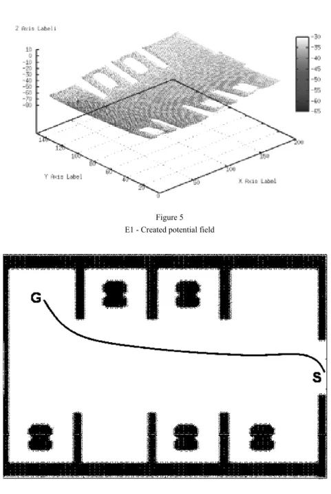
Using knowledge about the structure of a given car park and current occupation of individual parking boxes, see Fig. 4, (sensed by a type of appropriate sensors, e.g. cameras) a potential field is created, see Fig. 5. At this moment we suppose, the whole area is static (maybe it will also stay static). Then a vector field is computed. After determination of the starting point we will get the resulting path (the safest and shortest), see Fig. 6, and the robot will start its motion. In each sampling step it is controlled by the neural networks and also the situation in the car park is observed. There are controlled the turning angle and acceleration. If the environment stays static then control will continue by the neural network if no then the control will be switched to the fuzzy controller. It uses principles of sonar perception, detailed described in [7]. Its use is necessary if the obstacle intersects the computed path. The controller has two particular tasks, which are solved simultaneously: obstacle avoidance and searching for orientation marks. They issue to bringing the robot again to orientation marks. After that the control is again switched to the neural network. The whole process can be seen in the environment of a simulator, Figs. 7 and 11.

4 Experiments

Here two experiments will be described. The first one E1 can be seen in Figs. 4-7 and the simulation of the second one E2 in Fig. 11. Three basic characteristics were observed in dependence of sampling steps: control type, turning angle and acceleration.

Figure 4

E1 - Sensed situation of the car park

Figure 5 E1 - Created potential field

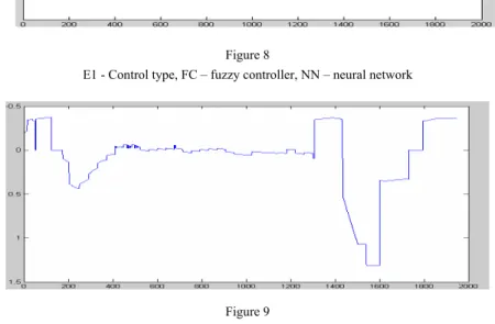
Figure 6

E1 - Computed path form the starting point S to the goal G

Figure 7

E1 - Simulated navigation in static environment

Figure 8

E1 - Control type, FC – fuzzy controller, NN – neural network

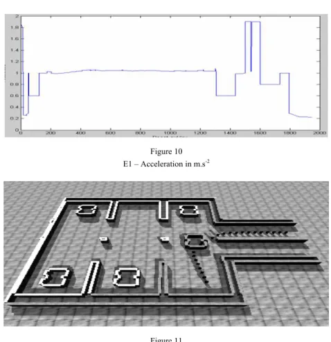
Figure 10 E1 – Acceleration in m.s-2

Figure 11

E2 - Simulated navigation in dynamic environment

Figure 12

E2 - Control type, FC – fuzzy controller, NN – neural network

Changes of the control type occur also in the experiment E1, i.e. not only during avoidance of a dynamic obstacle as mentioned in above. This state arises always when the robot approaches to an obstacle too close or robot sensors lose the contact with orientation marks for a while then the situation will be evaluated as a dynamic obstacle and the fuzzy controller will take over the control.

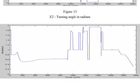
Figure 13 E2 - Turning angle in radians

Figure 14 E2 - Acceleration in m.s-2

Conclusions

The presented work had the aim to show the possibility of use harmonic potential fields together with systems of computational intelligence like fuzzy controllers and neural networks. All three approaches are based on numerical calculations and all three ones are derived from metaphors existing in the real world. The aim of this paper is also to contribute to discussions about using the so-called ‘dirty’ methods in artificial intelligence, whether yes or no. The answer in the opinion of the author is unambiguously ‘yes’.

• Design of methods for quicker constructing of potential fields.

• Modification of computation methods for handling only such area parts, which are necessary for trajectory design.

• Using previous two points in such a manner, which would reinforce the computational efficiency and thereby it would be possible directly to implement potential fields into environments with dynamic obstacles and to recalculate them in each time step [2].

• Design of functions for constructing potential fields, which could not cause rapid decrease of values in the vector field.

• More sophisticated switching between various controllers to eliminate the effect of chattering.

• Design of further approaches (also based on heuristics) being able to solve more complicated situations and various ‘traps’.

References

[1] Barrett, R. at al.: Templates for the Solution of Linear Systems: Building Blocks for Iterative Methods, 2nd ed., Philadelphia, PA: SIAM, 1994, (http://www.netlib.org/linalg/html_templates/Templates.html), ISBN 0-89871-328-5

[2] Bell, G., Weir, M. K.: Forward Chaining for Robot and Agent Navigation using Potential Fields, In: Proceedings of 27th Australasian Computer Science Conference (ACSC2004), Australian Computer Science Communications, Vol. 26, N. 1, Dunedin, New Zealand, pp. 265-274, ISBN 1-920682-05-8, ISSN 1445-1336, 2004

[3] Connolly, C. I.: Harmonic Functions and Collision Probabilities, In: Proceedings of the IEEE International Conference on Robotics & Automation (ICRA), pp. 3015-3019, 1994

[4] Dudek, G., Jenkin M.: Computational Principles of Mobile Robotics, Cambridge University Press, Cambridge, ISBN 0-521-56021-7, 2000

[5] Khatib, O.: Real-Time Obstacle Avoidance for Manipulators and Mobile Robots, In: Proceedings of IEEE International Conference onRobotics and Automation, Vol. 2, pp. 500-505, 1985

[6] Koditschek, D.: Exact Robot Navigation by Means of Potential Functions: Some Topological Considerations, In: Proceedings of the IEEE International Conference on Robotics and Automation, Vol. 4, pp. 1-6, 1987