A satellite data driven biophysical modeling approach for estimating northern peatland and tundra CO<sub>2</sub> and CH<sub>4</sub> fluxes

(1)

BGD

10, 16491–16549, 2013

A satellite data driven biophysical modeling

J. D. Watts et al.

Title Page

Abstract Introduction

Conclusions References

Tables Figures

◭ ◮

Back Close

Full Screen / Esc

Printer-friendly Version Interactive Discussion

Discussion

P

a

per

|

D

iscussion

P

a

per

|

Discussion

P

a

per

|

Discuss

ion

P

a

per

|

Biogeosciences Discuss., 10, 16491–16549, 2013 www.biogeosciences-discuss.net/10/16491/2013/ doi:10.5194/bgd-10-16491-2013

Open Access

Biogeosciences

Discussions

This discussion paper is/has been under review for the journal Biogeosciences (BG). Please refer to the corresponding final paper in BG if available.

A satellite data driven biophysical

modeling approach for estimating

northern peatland and tundra CO

₂

and

CH

4

fluxes

J. D. Watts1,2, J. S. Kimball1,2, F.-J. W. Parmentier3, T. Sachs4, J. Rinne5,

D. Zona6,7, W. Oechel7, T. Tagesson8, M. Jackowicz-Korczyński3, and M. Aurela9

1

Flathead Lake Biological Station, The University of Montana, 32125 Bio Station Lane, Polson, MT, USA

2

Numerical Terradynamic Simulation Group, CHCB 428, 32 Campus Drive, The University of Montana, Missoula, MT, USA

3

Department of Physical Geography and Ecosystem Science, Lund University, Sölvegatan 12, 223 62, Lund, Sweden

4

Helmholtz Centre Potsdam – GFZ German Research Centre for Geosciences, Telegrafenberg, 14473 Potsdam, Germany

5

Department of Physics, P.O. Box 48, 00014 University of Helsinki, Finland

6

Department of Animal and Plant Science, University of Sheﬃeld, Sheﬃeld, UK

7

(2)

BGD

10, 16491–16549, 2013

J. D. Watts et al.

Title Page

Tables Figures

◭ ◮

Back Close

Full Screen / Esc

Discussion

P

a

per

|

D

iscussion

P

a

per

|

Discussion

P

a

per

|

Discuss

ion

P

a

per

|

8

Department of Geography and Geology, University of Copenhagen, Øster Voldgade 10, 1350 København, Denmark

9

Finnish Meteorological Institute, Climate Change Research, P.O. Box 503, 00101, Helsinki, Finland

Received: 5 September 2013 – Accepted: 11 October 2013 – Published: 25 October 2013

Correspondence to: J. D. Watts (jennifer.watts@ntsg.umt.edu)

(3)

BGD

10, 16491–16549, 2013

J. D. Watts et al.

Title Page

Tables Figures

◭ ◮

Back Close

Full Screen / Esc

Discussion

P

a

per

|

D

iscussion

P

a

per

|

Discussion

P

a

per

|

Discuss

ion

P

a

per

|

Abstract

The northern terrestrial net ecosystem carbon balance (NECB) is contingent on in-puts from vegetation gross primary productivity (GPP) to oﬀset ecosystem respiration (R_eco) of carbon dioxide (CO₂) and methane (CH₄) emissions, but an e_ﬀective frame-work to monitor the regional Arctic NECB is lacking. We modified a terrestrial car-5

bon flux (TCF) model developed for satellite remote sensing applications to estimate peatland and tundra CO₂ and CH₄ fluxes over a pan-Arctic network of eddy covari-ance (EC) flux tower sites. The TCF model estimates GPP, CO2 and CH4 emissions

using either in-situ or remote sensing based climate data as input. TCF simulations driven using in-situ data explained>70 % of ther2variability in 8 day cumulative EC 10

measured fluxes. Model simulations using coarser satellite (MODIS) and reanalysis (MERRA) data as inputs also reproduced the variability in the EC measured fluxes rel-atively well for GPP (r2=0.75),R_eco (r2=0.71), net ecosystem CO₂ exchange (NEE,

r2=0.62) and CH4 emissions (r 2

=0.75). Although the estimated annual CH4

emis-sions were small (<18 g C m−2yr−1) relative toReco (>180 g C m

−2

yr−1), they reduced 15

the across-site NECB by 23 % and contributed to a global warming potential of ap-proximately 165±128 g CO₂eq m−2yr−1when considered over a 100 yr time span. This

model evaluation indicates a strong potential for using the TCF model approach to doc-ument landscape scale variability in CO2 and CH4 fluxes, and to estimate the NECB

for northern peatland and tundra ecosystems. 20

1 Introduction

Northern peatland and tundra ecosystems are important components of the terrestrial carbon cycle and store over half of the global soil organic carbon reservoir in seasonally frozen and permafrost soils (Hugelius et al., 2013). However, these systems are be-coming increasingly vulnerable to carbon losses as carbon dioxide (CO₂) and methane 25

(4)

BGD

10, 16491–16549, 2013

J. D. Watts et al.

Title Page

Tables Figures

◭ ◮

Back Close

Full Screen / Esc

Discussion

P

a

per

|

D

iscussion

P

a

per

|

Discussion

P

a

per

|

Discuss

ion

P

a

per

|

balance (Kane et al., 2012; Kim et al., 2012) that can increase soil carbon decompo-sition. Recent net CO2 exchange in northern tundra and peatland ecosystems varies

from a sink of 291 Tg C yr−1to a source of 80 Tg C yr−1, when considering the substan-tial uncertainty in regional estimates using scaled flux observations, atmospheric inver-sions, and ecosystem process models (McGuire et al., 2012). The magnitude of carbon 5

sink largely depends on the balance between carbon uptake by vegetation productivity and losses from soil mineralization and respiration processes. High latitude warming can increase ecosystem carbon uptake by reducing cold-temperature constraints on plant carbon assimilation and growth (Hudson et al., 2011; Elmendorf et al., 2012). Soil warming also accelerates carbon losses due to the exponential eﬀects of temper-10

ature on soil respiration, whereas wet and inundated conditions shift microbial activity towards anaerobic consumption pathways that are relatively slow but can result in sub-stantial CH4production (Moosavi and Crill, 1997; Merbold et al., 2009). Regional

wet-ting across the Arctic (Watts et al., 2012; Zhang et al., 2012a) may increase CH₄ emis-sions, which have a radiative warming potential at least 25 times more potent than CO2

15

per unit mass over a 100 yr time horizon (Boucher et al., 2009). The northern latitudes already contain over 50 % of global wetlands and recent increases in atmospheric CH₄ concentrations have been attributed to heightened gas emissions in these areas during periods of warming (Dlugokencky et al., 2009; Dolman et al., 2010). Northern peatland and tundra (≥50◦N) reportedly contribute between 8–79 Tg C in CH₄ emissions each

20

year, but these fluxes have been diﬃcult to constrain due to uncertainty in the param-eterization of biogeochemical models, the regional characterization of wetland extent and water table depth, and a scarcity of ecosystem scale CH₄ emission observations (Petrescu et al., 2010; Riley et al., 2011; Spahni et al., 2011; McGuire et al., 2012; Meng et al., 2012).

25

Ecosystem studies using chamber and eddy covariance (EC) methods continue to provide direct measurements of CO2 and CH4fluxes and add valuable insight into the

(5)

BGD

10, 16491–16549, 2013

J. D. Watts et al.

Title Page

Tables Figures

◭ ◮

Back Close

Full Screen / Esc

Discussion

P

a

per

|

D

iscussion

P

a

per

|

Discussion

P

a

per

|

Discuss

ion

P

a

per

|

extremely sparse in-situ monitoring network and the large spatial extent and hetero-geneity of peatland and tundra ecosystems. Recent approaches have used satellite-based land cover classifications, photosynthetic leaf area maps, or wetness indices to “up-scale” CO2 (Forbrich et al., 2011; Marushchak et al., 2013) and CH4 (Tagesson

et al., 2013; Sturtevant and Oechel, 2013) flux measurements. Remote sensing in-5

puts have also been used in conjunction with biophysical process modeling to estimate landscape-level changes in plant carbon assimilation and soil CO2 emissions (Yuan

et al., 2011; Tagesson et al., 2012a; Yi et al., 2013). Previous analyses of regional CH4

emissions have ranged from the relatively simple modification of CH₄ emission rate estimates for wetland fractions according to temperature and carbon substrate con-10

straints (Potter et al., 2006; Clark et al., 2011) or the use of more complex multi-layer wetland CH₄ models with integrated hydrological components (McGuire et al., 2012; Wania et al., 2013). Yet, most investigations have not examined the potential for si-multaneously assessing CO2 and CH4 fluxes, and the corresponding net ecosystem

carbon balance (NECB; Sitch et al., 2007; Olefeldt et al., 2012; McGuire et al., 2012) 15

for peatland and tundra using a satellite remote sensing based model approach. It is well recognized that sub-surface conditions influence the land-atmosphere ex-change of CO₂and CH₄production. However, near-surface soil temperature, moisture and carbon substrate availability play a crucial role in regulating ecosystem carbon emissions. Strong associations between surface soil temperature (≤10 cm depth) and 20

CO₂respiration have been observed in Arctic peatland and tundra permafrost systems (Kutzbach et al., 2007). Significant relationships between CH4emissions and

tempera-ture have also been reported (Hargreaves et al., 2001; Zona et al., 2009; Sachs et al., 2010). Although warming generally increases the decomposition of organic carbon, the magnitude of CO2production is constrained by wet soil conditions (Olivas et al., 2010)

25

which instead favor CH4emissions and decrease methantrophy in soil and litter layers

(Turetsky et al., 2008; Olefeldt et al., 2012). Oxidation by methanotrophic communities in surface soils can reduce CH4 emissions by over 90 % when gas transport occurs

(6)

BGD

10, 16491–16549, 2013

J. D. Watts et al.

Title Page

Tables Figures

◭ ◮

Back Close

Full Screen / Esc

Discussion

P

a

per

|

D

iscussion

P

a

per

|

Discussion

P

a

per

|

Discuss

ion

P

a

per

|

water content rises above 55–65 % (von Fischer and Hedin, 2007; Sjögersten and Wookey, 2009). Despite increases in the availability of organic carbon and accelerated CO2 release due to increased soil temperature and thickening of the active layer in

permafrost soils (Dorrepaal et al., 2009), anaerobic communities have shown a prefer-ence for light-carbon fractions (e.g. amines, carbonic acids) that are more abundant in 5

the upper soil horizons (Wagner et al., 2009). Similarly, labile carbon substrates from recent photosynthesis and root exudates have been observed to increase CH₄ pro-duction relative to heavier organic carbon fractions (Ström et al., 2003; Dijkstra et al., 2012; Olefeldt et al., 2013).

The objective of this study was to evaluate the feasibility of using a satellite remote 10

sensing data driven modeling approach to assess the daily and seasonal variability in CO2 and CH4 fluxes from northern peatland and tundra ecosystems, according to

near-surface environmental controls including soil temperature, moisture and available soil organic carbon. In this paper we incorporate a newly developed CH₄ emissions algorithm within an existing Terrestrial Carbon Flux (TCF) CO2model framework

(Kim-15

ball et al., 2012; Yi et al., 2013). The CH4emissions algorithm simulates gas production

using near-surface temperature, anaerobic soil fractions and labile organic carbon as inputs. Plant CH4transport is determined by vegetation growth characteristics derived

from gross primary production (GPP), plant functional traits and canopy/surface turbu-lence. Methane di_ﬀusion is determined based on temperature and moisture constraints 20

to gas movement through the soil column, and oxidation potential. Ebullition of CH4is

assessed using a simple gradient method (van Huissteden et al., 2006).

The integrated TCF model framework allows for satellite remote sensing information to be used as primary inputs and requires minimal parameterization relative to more complex ecosystem process models. It also provides an initial step towards the re-25

(7)

BGD

10, 16491–16549, 2013

J. D. Watts et al.

Title Page

Tables Figures

◭ ◮

Back Close

Full Screen / Esc

Discussion

P

a

per

|

D

iscussion

P

a

per

|

Discussion

P

a

per

|

Discuss

ion

P

a

per

|

other mechanisms of carbon transport, including dissolved and volatile organic carbon emissions and fire-based particulates, the NECB is limited in this study to terrestrial CO2 and CH4 fluxes, which often are primary contributors in high latitude tundra and

peatland ecosystems (McGuire et al., 2010).

To evaluate the combined CO2 and CH4 algorithm approach, we compared TCF

5

model simulations to tower EC records from six northern peatland and tundra sites within North America and Eurasia. For this study, baseline TCF simulations driven with tower EC based GPP and in-situ meteorology data were first used to assess the ca-pability of the TCF model approach to quantify temporal changes in landscape scale carbon (CH₄and CO₂) fluxes. Secondly, CO₂and CH₄simulations using internal TCF 10

model GPP estimates (Yi et al., 2013) and inputs from satellite and global model re-analysis records were used to evaluate the relative uncertainty introduced when driving the model using coarser scale information in place of in-situ data. These satellite and reanalysis driven TCF simulations were then used to evaluate annual CO₂ and CH₄ fluxes at the six tower sites, and the relative impact of CH4emissions on the NECB.

15

2 Methods

2.1 TCF model description

The combined TCF CO₂ and CH₄ flux model framework regulates carbon gas ex-change using soil surface temperature, moisture and soil organic carbon availability as inputs, and has the flexibility to run simulations at local and regional scales. TCF model 20

estimates of ecosystem respiration (R_eco) and net ecosystem CO₂exchange (NEE) at a daily time step have been evaluated against tower EC datasets from boreal and tun-dra systems using GPP, surface (≤10 cm depth) soil temperature (Ts) and volumetric

moisture content (θ) inputs available from global model reanalysis and satellite remote sensing records (Kimball et al., 2009; McGuire et al., 2012). A recent adjustment to 25

(8)

BGD

10, 16491–16549, 2013

J. D. Watts et al.

Title Page

Tables Figures

◭ ◮

Back Close

Full Screen / Esc

Discussion

P

a

per

|

D

iscussion

P

a

per

|

Discussion

P

a

per

|

Discuss

ion

P

a

per

|

(LUE) algorithm that provides internally derived GPP calculations to determineR_eco

and NEE fluxes. The adjusted TCF CO2model also allows for better user control over

parameter settings and surface meteorological inputs (Kimball et al., 2012). The TCF CO₂and newly added CH₄flux model components are described in the following sec-tions. A summary of the TCF model inputs, parameters, and the associated parameter 5

values used in this study is provided in the Supplement (Tables S1 and S2; Fig. S1).

2.1.1 CO2flux component

The internal TCF LUE algorithm estimates daily GPP fluxes according to a biome-dependent vegetation maximum LUE coeﬃcient (εmax; mg C MJ

−1

) which represents the optimal conversion of absorbed solar energy and CO₂ to plant organic carbon 10

through photosynthesis (Kimball et al., 2012). To account for environmental constraints on photosynthesis,εmaxis reduced (ε) using dimensionless linear rate scalars ranging

from 0 (total inhibition) to 1 (no inhibition) that are described elsewhere (i.e. Kimball et al., 2012; Yi et al., 2013). Following the approach of Running et al. (2004), daily min-imum air temperature (Tmin) and atmospheric vapor pressure deficit (VPD) are used

15

to define the environmental constraints on GPP. In this study we include a constraint based on θ to account for the sensitivity of bryophytes and shallow rooted species to surface drying (Wu et al., 2013), where θmin and θmax are specified minimum and

maximum parameter values: ε=εmax×f(VPD)×f(Tmin)×f(θ)

wheref(θ)=(θ−θ_min)/(θmax−θmin).

(1) 20

Simulated GPP (g C m−2d−1) is obtained as:

GPP =ε×0.45 SWrad× FPAR (2)

where SWrad(W m

−2

(9)

BGD

10, 16491–16549, 2013

J. D. Watts et al.

Title Page

Tables Figures

◭ ◮

Back Close

Full Screen / Esc

Discussion

P

a

per

|

D

iscussion

P

a

per

|

Discussion

P

a

per

|

Discuss

ion

P

a

per

|

2005). Remotely sensed normalized diﬀerence vegetation index (NDVI) records have been used to estimate vegetation productivity (Schubert et al., 2010a; Parmentier et al., 2013) and changes in growing season length (Beck and Goetz, 2011) across north-ern peatland and tundra environments. Daily FPAR is derived using the approach of Badawy et al. (2013) to mitigate potential biases in low biomass landscapes (Peng 5

et al., 2012):

FPAR =0.94(Index − Indexmin)

Indexrange

(3)

This approach uses NDVI or simple ratio (SR; i.e. (1+NDVI)/(1−NDVI)) indices as input Index values. The results are then averaged to obtain FPAR. Indexrange

corre-sponds to the diﬀerence between the 2nd and 98th percentiles in the NDVI and SR 10

distributions (Badawy et al., 2013).

Biome-specific autotrophic respiration (Ra) is estimated using a carbon use eﬃ

-ciency (CUE) approach that considers the ratio of net primary production (NPP) to GPP (Choudhury, 2000). Carbon loss from heterotrophic respiration (Rh) is determined

us-ing a 3-pool soil litter decomposition scheme consistus-ing of metabolic (Cmet), structural

15

(C_str) and recalcitrant (C_rec) organic carbon pools with variable decomposition rates. TheCmetpool represents easily decomposable plant residue and root exudates

includ-ing amino acids, sugars and simple polysaccharides, whereas theCstr pool consists

of more recalcitrant litter residue such as hemi-cellulose and lignin (Ise et al., 2008; Porter et al., 2010). TheCrecpool includes physically and chemically stabilized carbon

20

derived from theCmetandCstrpools and also corresponds to humified peat. A fraction

of daily NPP (F_met) is first allocated as readily decomposable litterfall toC_met and the remaining portion (1−Fmet) is transferred toCstr(Ise and Moorcroft, 2006; Kimball et al.,

2009). To account for reduced mineralization in tundra and peatland environments, ap-proximately 70 % ofCstr(Fstr) is reallocated toCrec(Ise and Moorcroft, 2006; Ise et al.,

(10)

BGD

10, 16491–16549, 2013

J. D. Watts et al.

Title Page

Tables Figures

◭ ◮

Back Close

Full Screen / Esc

Discussion

P

a

per

|

D

iscussion

P

a

per

|

Discussion

P

a

per

|

Discuss

ion

P

a

per

|

2008):

dCmet/dt= NPP ×Fmet−Rh, met (4)

dCstr/dt= NPP (1−Fmet)−(Fstr×Cstr)−Rh, str (5)

dC_rec/dt₌(F_str×C_str)−R_{h, rec} (6)

5

CO2loss fromCmet(Rh, met) is determined using an optimal decomposition rate

param-eter (K_p) that is attenuated (K_met) by dimensionless T_s and θbased multipliers (T_mult

andWmult, respectively) constrained between 0 and 1 to account for the reduced

de-composition of soil organic carbon due to environmental conditions:

K_met=K_p×T_mult×W_mult (7)

10

Tmult=exp

h

308.5666.02−1

−(Ts+Tref−66.17)

−1i

(8)

Wmult=1−2.2(θ−θopt)2 (9)

The cold temperature constraints are imposed using an Arrhenius-type function (Lloyd and Taylor, 1994; Kimball et al., 2009) where decomposition is no longer limited when 15

average dailyTsexceeds a user-specified reference temperature (Tref; in K) which can

vary with carbon substrate complexity, physical protection, oxygen availability and water stress (Davidson and Janssens, 2006). TheWmult modifier accounts for the inhibitory

eﬀect of dry and near-saturated soil moisture conditions on heterotrophic decomposi-tion (Oberbauer et al., 1996). For this study, θopt is set to 80 % of pore saturation to

20

account for ecosystem adaptations to wet soil conditions (Ise et al., 2008; Zona et al., 2012) and near-surface oxygen availability provided by plant root transport (Elberling et al., 2011). Decomposition rates forC_strandC_rec(K_str,K_rec) are determined as 40 % and 1 % ofKmet, respectively (Kimball et al., 2009), andRh is the total CO2loss from

the three soil organic carbon pools: 25

(11)

BGD

10, 16491–16549, 2013

J. D. Watts et al.

Title Page

Tables Figures

◭ ◮

Back Close

Full Screen / Esc

Discussion

P

a

per

|

D

iscussion

P

a

per

|

Discussion

P

a

per

|

Discuss

ion

P

a

per

|

Finally, the TCF model estimates NEE (g C m−2d−1) as the residual diﬀerence between

Reco, which includes Ra and Rh respiration components, and GPP. Negative (−) and

positive (₊) NEE fluxes denote respective terrestrial CO₂sink and source activity:

NEE =(R_a+R_h)−GPP (11)

2.1.2 CH4flux component 5

A CH4 emissions algorithm was incorporated within the TCF model to estimate CH4

fluxes for peatland and tundra landscapes. The modified TCF model estimates CH4

production according to T_s, θ, and labile carbon availability. Plant CH₄ transport is modified by vegetation growth and production, plant functional traits, and canopy aero-dynamic conductance which takes into account the influence of wind turbulence on 10

moisture/gas flux between vegetation and the atmosphere. The TCF-CH₄ structure is similar to other process models (e.g. Walter and Heimann, 2000; van Huissteden et al., 2006) but reduces to a one-dimensional near-surface soil profile following Tian et al. (2010) to simplify model parameterization amenable to remote sensing applica-tions. For the purposes of this study, the soil profile is defined for surface (≤10 cm 15

depth) soil layers as most temperature and moisture retrievals from satellite remote sensing and reanalysis records do not characterize deeper soil conditions. Although this approach may not account for variability in carbon fluxes associated with deeper soil constraints, field studies from high latitude ecosystems have reported strong as-sociations between CH₄ emissions and near-surface conditions including T_s and soil 20

moisture (Hargreaves et al., 2001; Sachs et al., 2010; von Fischer et al., 2010; Sturte-vant et al., 2012; Tagesson et al., 2012b).

CH4production

Soil moisture in the upper rhizosphere is a fundamental control on CH₄production and emissions to the atmosphere. Methanogenesis (RCH₄) within the saturated soil pore

(12)

BGD

10, 16491–16549, 2013

J. D. Watts et al.

Title Page

Tables Figures

◭ ◮

Back Close

Full Screen / Esc

Discussion

P

a

per

|

D

iscussion

P

a

per

|

Discussion

P

a

per

|

Discuss

ion

P

a

per

|

volume (φs; m

−3

; aerated pore volume is denoted as φa) is determined according to

an optimal CH₄production rate (R_o; µM CH₄d−1) and labile photosynthates:

RCH₄=(Ro×φs)×Cmet×Q

(T_s−T_p)/10

10p (12)

For this study, CH4production was driven using the less recalcitrantCmetpool to reflect

contributions by lower weight carbon substrates (Reiche et al., 2010; Corbett et al., 5

2012) in labile organic carbon-rich environments. Carbon contributions from theC_str

pathway may also be allocated for CH4 production in ecosystems with lower labile

organic carbon inputs and higher contributions by hydrogenotrophic methanogenesis (Alstad and Whiticar, 2011). TheQ₁₀_ptemperature modifier is used as an approxima-tion to the Arrhenius equaapproxima-tion and describes the temperature dependence of biological 10

processes (Gedney and Cox, 2003; van Huissteden et al., 2006). The reference tem-perature (Tp) typically reflects mean annual or non-frozen season climatology. Both

Q₁₀_pand T_p can be adjusted, in addition toR_o, to accommodate varying temperature sensitivities in response to ecosystem diﬀerences in substrate quality and other envi-ronmental conditions (van Hulzen et al., 1999; Inglett et al., 2012). Methane additions 15

fromR_CH

4are first allocated to a temporary soil CH4storage pool (CCH4) prior to

deter-mining the CH4emissions for each 24 h time step;Cmet is also updated to account for

carbon losses due to CH4production.

CH4emission

The magnitude of daily CH₄emissions (F_total) from the soil profile is determined through 20

plant transport (Fplant), soil diﬀusion (Fdiﬀ) and ebullition (Febull) pathways:

Ftotal=Fplant+Fdiﬀ+Febull (13)

(13)

BGD

10, 16491–16549, 2013

J. D. Watts et al.

Title Page

Tables Figures

◭ ◮

Back Close

Full Screen / Esc

Discussion

P

a

per

|

D

iscussion

P

a

per

|

Discussion

P

a

per

|

Discuss

ion

P

a

per

|

and often reducing the degree of CH₄ oxidation (Joabsson et al., 1999). DailyF_plantis determined using a rate constant (Cp) modified by vegetation growth and production

(fgrow), an aerodynamic term (λ) and a rate scalar (Ptrans) that account for diﬀerences

in CH₄transport ability according to plant functional type:

Fplant=(CCH₄×Cp×fgrow×λ×Ptrans)(1−Pox) (14)

5

A fraction ofFplant is oxidized (Pox) prior to reaching the atmosphere and can be

mod-ified according to plant functional characteristics (Frenzel and Rudolph, 1998; Ström et al., 2005; Kip et al., 2010). Plant transport is further reduced under frozen surface conditions to account for pathway obstruction by ice and snow or bending of the plant stem following senescence (Hargreaves et al., 2001; Sun et al., 2012). The magnitude 10

off_grow is determined as the ratio of daily GPP to its annual maximum and is used to account for seasonal diﬀerences in root and above-ground biomass (Chanton, 2005).

Aerodynamic conductance (ga) represents the influence of near-surface turbulence

on energy/moisture fluxes between vegetation and the atmosphere (Roberts, 2000; Yan et al., 2012) and gas transport within the plant body (Sachs et al., 2008; Wegner 15

et al., 2010; Sturtevant et al., 2012):

g_a₌ k

2

µm

ln[(zm−d)/zom] ln[(zm−d)/zov]

(15)

Values for z_m and d are the respective anemometer and zero plane displacement heights (m); zom and zov are the corresponding roughness lengths (m) for

momen-tum, heat and vapor transfer. The von Karman constant (k; 0.40) is a dimensionless 20

constant in the logarithmic wind velocity profile (Högström, 1988),µm is average daily

wind velocity (m s−1), d is calculated as 2/3 of the vegetation canopy height, z_om is roughly 1/8th of canopy height (Yang and Friedl, 2002), and zov is 0.1zom(Yan et al.,

2012). Estimatedga is scaled between 0 and 1 to obtainλusing a linear function for

(14)

BGD

10, 16491–16549, 2013

J. D. Watts et al.

Title Page

Tables Figures

◭ ◮

Back Close

Full Screen / Esc

Discussion

P

a

per

|

D

iscussion

P

a

per

|

Discussion

P

a

per

|

Discuss

ion

P

a

per

|

a higher sensitivity to surface turbulence, a quadratic approach is used whenµm

ex-ceeds 4 m s−1:

λ=0.0246+0.5091ga

λ=0.0885−(3.28g_a)+

44.51g_a2,µm>4 m s

−1 (16)

Although this approach focuses on the influence of wind turbulence on plant gas trans-port within vegetated wetlands, it is also applicable for inundated microsites where 5

increases in surface water mixing can stimulate CH4 degassing (Sachs et al., 2010).

In addition, Eq. (15) reflects near-neutral atmospheric stability and adjustments may be necessary to accommodate unstable or stable atmospheric conditions (Raupach, 1998).

The upward diﬀusion of CH4 within the soil profile is determined using a

one-10

layer approach similar to Tian et al. (2010). The rate of CH₄ transport (D_e; m−2d−1) is considered for both saturated (Dwater; 1.73×10

−4

µM CH4d

−1

) and aerated (Dair;

1.73 µM CH4d

−1

) soil fractions:

De=(Dwater×φs)(Dair×φa) (17)

Potential daily transport through di_ﬀusion (P_di_ﬀ) is estimated as the product ofD_e and 15

the gradient between CCH₄and the atmospheric CH4 concentration (AirCH₄). This is

further modified by soil tortuosity (τ; 0.66), which increases exponentially forTs<274 K

to account for slower gas movement at colder temperatures and barriers to di_ﬀusion resulting from near-surface ice formation (Walter and Heimann, 2000; Zhuang et al., 2004), and pathway constraints within the saturated pore fraction (1−θ):

20

Pdiﬀ=τ×De(CCH₄−AirCH₄)(1−θ)

Ts≥274, τ=0.66

Ts<274, τ=0.05+10

−238

×Ts97.2

(15)

BGD

10, 16491–16549, 2013

J. D. Watts et al.

Title Page

Tables Figures

◭ ◮

Back Close

Full Screen / Esc

Discussion

P

a

per

|

D

iscussion

P

a

per

|

Discussion

P

a

per

|

Discuss

ion

P

a

per

|

A portion of diﬀused CH₄ is oxidized (R_ox) before reaching the soil surface, using a Michaelis–Menten kinetics approach scaled byφa:

Rox=

(V_max×φ_a)P_di_ﬀ

(Km+φa)Pdi_ﬀ

×Q(Ts−Td)/10

10d (19)

where Vmax is the maximum reaction rate and Km is the substrate concentration at

0.5Vmax (van Huissteden et al., 2006). Oxidation during soil diﬀusion is modified by

5

soil temperatureQ₁₀ constraints (Q₁₀_d); T_d is the reference temperature and can be defined using site-specific mean annualTs(Le Mer and Roger, 2001). Total daily CH4

emission (Fdiﬀ) from the soil diﬀusion pathway is determined by substracting Rox from

P_di_ﬀ.

The TCF CH₄ algorithm uses a gradient-based approach to account for slow or 10

“steady-rate” ebullition from inundated micro-sites in the landscape (Rosenberry et al., 2006; Wania et al., 2010), whereas episodic events originating deeper within the soil re-quire more complex modeling techniques and input data rere-quirements (Kettridge et al., 2011) that are beyond the scope of this study. Emission contributions due to ebullition occur when CCH₄ exceeds a threshold value (ve) of 500 µM (van Huissteden et al.,

15

2006). The magnitude of gas release is determined by steady-rate bubbling (C_e) ap-plied within the saturated soil pore space (φs):

Febull=(Ce×φs) (CCH₄−υe),CCH₄ >ve (20)

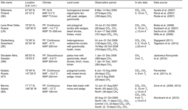
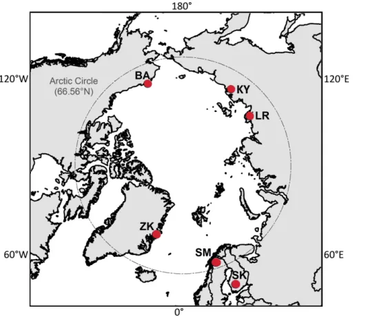
2.2 Study sites and in-situ data records

Tower EC records from six peatland and tundra sites in Finland, Sweden, Russia, 20

(16)

BGD

10, 16491–16549, 2013

J. D. Watts et al.

Title Page

Tables Figures

◭ ◮

Back Close

Full Screen / Esc

Discussion

P

a

per

|

D

iscussion

P

a

per

|

Discussion

P

a

per

|

Discuss

ion

P

a

per

|

collected near Chokurdakh in northeastern Siberia. The Zackenberg (ZK) flux tower is located within Northeast Greenland National Park, and tower data records for Alaska were obtained from a water table manipulation experiment (Zona et al., 2009, 2012; Sturtevant et al., 2012) located approximately 6 km east of Barrow (BA). With excep-tion of Siikaneva, the EC tower footprints represent wet permafrost ecosystems with 5

complex, heterogeneous terrain that includes moist depressions, drier, elevated hum-mocks and inundated microsites. Vegetation within the tower footprints (Rinne et al., 2007; Riutta et al., 2007; Sachs et al., 2008; Jackowicz-Korczyński et al., 2010; Par-mentier et al., 2011a; Zona et al., 2011; Tagesson et al., 2012b) consists of Carex

and other sedges, dwarf shrubs (e.g.DryasandSalix), grasses (e.g.Arctagrostis) and 10

Sphagnummoss (with exception of Zackenberg).

For Siikaneva,Ts records from 5 and 10 cm depths were obtained for this analysis,

but only water table depth information was available to describe soil wetness (Rinne et al., 2007). At the Lena River siteT_s (5, 10 cm) andθ (≤12 cm) observations were

obtained from the nearby Samoylov meteorological station and represent tundra poly-15

gon wet center, dry rim and slope conditions (Boike et al., 2008; Sachs et al., 2008). Althoughθwas also measured during summer 2006 the records are limited to the wet polygon center location (J. Boike, personal communication, 2012) and were not used in this study due to the potential for overestimating saturated site conditions and cor-responding CH₄ fluxes. For Zackenberg, in-situ T_s measurements were obtained for 20

the 2 cm depth (Tagesson et al., 2012a, b) within the tower footprint; near-surfaceθ (<20 cm) and 5 and 10 cmTsmeasurements were collected adjacent to the site

(Sigs-gaard et al., 2011). At Stordalen Mire, in-situ θ was not available at the time of this study andTs measurements were only for the 3 cm depth (Jackowicz-Korczyński et al.,

2010). In-situ θ was also not collected at Kytalyk but Ts was obtained for the 4 cm

25

(17)

BGD

10, 16491–16549, 2013

J. D. Watts et al.

Title Page

Tables Figures

◭ ◮

Back Close

Full Screen / Esc

Discussion

P

a

per

|

D

iscussion

P

a

per

|

Discussion

P

a

per

|

Discuss

ion

P

a

per

|

locations within the Barrow tower footprints, but in 2009 T_s was only available at the 5 cm depth. For Barrow (2007), only CO2 and CH4 EC measurements corresponding

to the north tower were used in the analysis, due to minimal EC data availability for the south and central tower sites following flux processing (Zona et al., 2009). Many of the Barrow CO2measurements were also rejected during data processing for the 2009

5

period; as a result NEE was not partitioned intoRecoand GPP (Sturtevant et al., 2012).

2.3 Remote sensing and reanalysis inputs

Daily input meteorology was obtained from the Goddard Earth Observing System Data Assimilation Version 5 (GEOS-5) MERRA archive (Rienecker et al., 2011) with 1/2×2/3◦spatial resolution. The MERRA records were recently verified for terrestrial 10

CO₂applications in high latitude systems (Yi et al., 2011, 2013; Yuan et al., 2011), and provide model enhancedTsand surface θinformation similar to the products planned

for the NASA SMAP mission (Kimball et al., 2012). In addition to near surface (≤10 cm)

T_sandθinformation from the MERRA-Land reanalysis (Reichle et al., 2011) required for theReco and CH4 simulations, daily MERRA SWrad, Tmin and VPD records were

15

used to drive the internal TCF LUE model GPP calculations. The MERRA near-surface (2 m) wind parameters were also used to obtain mean dailyµ_m for the CH₄simulation estimates. The MERRA-Land records for Greenland are spatially limited due to land cover/ice masking inherent in the reanalysis product, and MERRATs andθwere not

available for the Zackenberg tower site. As a proxy,Ts was derived from MERRA

sur-20

face skin temperatures by applying a simple Crank–Nicholson heat di_ﬀusion scheme which accounts for energy attenuation with increasing soil depth (Wania et al., 2010); forθ, records from a nearby grid cell were used to represent moisture conditions at Zackenberg.

For the daily TCF LUE-based GPP simulations, quality screened cloud-filtered 16 day 25

(18)

BGD

10, 16491–16549, 2013

J. D. Watts et al.

Title Page

Tables Figures

◭ ◮

Back Close

Full Screen / Esc

Discussion

P

a

per

|

D

iscussion

P

a

per

|

Discussion

P

a

per

|

Discuss

ion

P

a

per

|

MYD13Q1 retrievals were minimal at the tower locations, and the combination of Terra and Aqua MODIS records reduced the retrieval gaps to approximate 8 day intervals. Linear interpolation was then used to scale the 8 day NDVI records to daily observa-tions. The NDVI retrievals correspond to the center coordinate locations for each flux tower site. Coarser (500–1000 m resolution) NDVI records were not used in this study 5

due to the close proximity of water bodies at the tower sites, which can substantially reduce associated FPAR retrievals. In addition, 250 m MODIS vegetation indices have been reported to better capture the overall seasonal variability in tower EC flux records (Schubert et al., 2012).

2.4 TCF model parameterization 10

A summary of the site specific TCF model parameters is provided in the Supplement (Table S2). Parameter values associated with grassland biomes were selected for the LUE model VPD and Tmin modifiers used to estimate GPP (Yi et al., 2013), as more

specific values for tundra and moss-dominated wetlands were not available. Parameter values forθmax were obtained using growing-season maximum θ measurements for

15

each site andθmin was set to 0.15 for scaling purposes. Modelεmaxwas specified as

0.82 mg C MJ−1 for the duration of the growing season, although actual LUE can vary throughout the summer due to diﬀerences in vegetation growth phenology and nutrient availability (Connolly et al., 2009; King et al., 2011). Tundra CUE ranged from 0.45 to 0.55 (Choudhury, 2000); a lower CUE value of 0.35 was used for the moss-dominated 20

Siikaneva tower site due to a more moderate degree of carbon assimilation occurring in bryophytes, that has been observed in other sub-Arctic communities (Street et al., 2012). For the TCF modelFmet parameter, the percentage of NPP allocated to Cmet

varied between 70 and 72 % for tower tundra sites (Kimball et al., 2009) compared to 50 and 65 % for Siikaneva and Stordalen Mire where moss cover is more abundant. 25

The TCF CH4moduleRoparameter ranged from 4.5 and 22.4 µM CH4d

−1

(Walter and Heimann, 2000; van Huissteden et al., 2006). Values forQ10p varied between 3.5 and

(19)

BGD

10, 16491–16549, 2013

J. D. Watts et al.

Title Page

Tables Figures

◭ ◮

Back Close

Full Screen / Esc

Discussion

P

a

per

|

D

iscussion

P

a

per

|

Discussion

P

a

per

|

Discuss

ion

P

a

per

|

conditions (Gedney and Cox, 2003; Inglett et al., 2012). AQ₁₀_d of 2 was assigned for CH4oxidation (Zhuang et al., 2004; van Huissteden et al., 2006). Parameter values for

Ptrans, which indicates relative plant transport ability, ranged from 7 to 9

(dimension-less); lower values were assigned to tower locations with a higher proportion of shrub and moss cover, whereas higher Ptrans corresponds to sites where sedges are more

5

prevalent (Ström et al., 2005; Rinne et al., 2007). Forλ, the scaled conductance for lower site wind sensitivity was used for the CH₄ simulations, with exception of Lena River which showed a higher sensitivity to surface turbulence. Values for Pox ranged

from 0.7 in tundra to 0.8 inSphagnum-dominated systems to account for higher CH4

oxidation by peat mosses (Parmentier et al., 2011c). Due to a lack of detailed soil profile 10

descriptions and heterogeneous tower footprints, soil porosity was assigned at 75 % for sites with more abundant fibrous surface layer peat (i.e. Siikaneva and Stordalen Mire) and 70 % elsewhere to reflect more humified or mixed organic and mineral surface soils (Elberling et al., 2008; Verry et al., 2011).

2.5 TCF model simulations 15

The TCF model was first evaluated against the tower EC records using simulations driven with in-situ measurement data including EC-based GPP, T_s, θ and µ_m inputs. This step allowed for baseline TCF modelR_ecoand CH₄flux estimates to be assessed without introducing additional input uncertainties from the coarser reanalysis meteorol-ogy records and TCF LUE model-derived GPP calculations. Site mean dailyTs andθ

20

measurement records corresponding to near-surface (≤10 cm) soil depths were used

for the TCF site based model simulations when possible, to better coincide with the soil penetration depths anticipated for upcoming satellite-based microwave remote sens-ing missions (Kimball et al., 2012). In addition to the TCF model runs ussens-ing site in-situ information, changes in temporal agreement and model uncertainty were evaluated for 25

simulations where MERRA based θ, Ts,µm, or TCF LUE GPP inputs were used in

(20)

BGD

10, 16491–16549, 2013

J. D. Watts et al.

Title Page

Tables Figures

◭ ◮

Back Close

Full Screen / Esc

Discussion

P

a

per

|

D

iscussion

P

a

per

|

Discussion

P

a

per

|

Discuss

ion

P

a

per

|

budgets for each site. Baseline carbon pools were initialized for each site by continu-ously cycling (“spinning-up”) the TCF model for the tower years of record (described in Table 1) to reach a dynamic steady-state between estimated NPP and surface soil organic carbon stocks (Kimball et al., 2009). In-situ data records were used during the model spin-up to establish baseline organic carbon conditions for the first five TCF 5

simulations, although it was often necessary to supplement these data with MERRA based information to obtain continuous annual time series. For the final model run, only MODIS and MERRA inputs were used during the spin-up process.

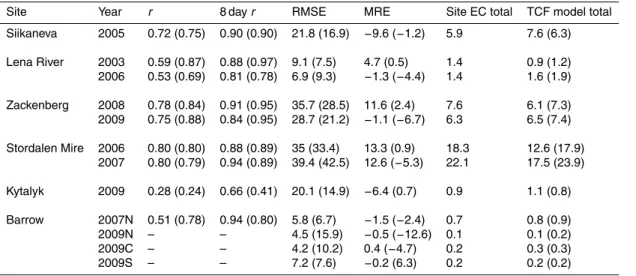
The temporal agreement between the tower EC records and TCF model simulations was assessed using Pearson correlation coeﬃcients (r;±one standard deviation) for

10

the daily, 8 day, and total-period (EC length of record) cumulative carbon fluxes and corresponding tests of significance at a 0.05 probability level. The 8 day and total-period cumulative fluxes were evaluated, in addition to the daily fluxes, to account for di_ﬀerences between the TCF model estimates and tower EC records stemming from temporal lags between changing environmental conditions and resulting carbon (CO2,

15

CH4) emissions (Lund et al., 2010; Levy et al., 2012). The mean residual error (MRE)

between the tower EC records and TCF modeled CO₂ and CH₄ fluxes was used to identify potential model biases; root-mean-square-error (RMSE) diﬀerences were used as a measure of model estimate uncertainty in relation to the tower EC records.

3 Results 20

3.1 Surface organic carbon pools

The TCF model-generated surface soil organic carbon pools represent steady-state conditions obtained through the continuous cycling of in-situ or MODIS and MERRA environmental inputs for the years of record associated with each tower site (described in Table 1). Approximately 600 and 1000 yr of spin-up by the TCF model were required 25

(21)

con-BGD

10, 16491–16549, 2013

J. D. Watts et al.

Title Page

Tables Figures

◭ ◮

Back Close

Full Screen / Esc

Discussion

P

a

per

|

D

iscussion

P

a

per

|

Discussion

P

a

per

|

Discuss

ion

P

a

per

|

ditions at the peatland and tundra sites, respectively, which is similar to previous sim-ulations conducted for northern EC tower locations (Kimball et al., 2009). The TCF model organic carbon pools are also comparable to northern soil carbon inventory records (Yi et al., 2013). Over 95 % of the resulting soil organic carbon pool was al-located to C_rec by the TCF model, with 2 to 3 % stored as C_met and the remainder 5

partitioned to Cstr. The estimated surface soil organic carbon pools from the in-situ

based TCF model spin-up ranged from ≃3.3 kg C m−2 for Zackenberg and Stordalen Mire and 1.1 to 1.5 kg C m−2for the other tower sites. The larger organic carbon stocks at Zackenberg reflect a combination of relatively high tower EC based GPP inputs, often exceeding 5 g C m−2d−1 during the peak growth season, and a relatively short 10

<50 day peak growing season (Tagesson et al., 2012a) that minimized TCF modeled

R_h losses. Although it was necessary to use internal LUE based GPP calculations for Stordalen Mire in the absence of available CO2records, the resulting TCF basedCmet

andCreccarbon stocks were similar in magnitude to plant litter measurements collected

at this site (Olsrud and Christensen, 2011). However, the TCF simulated soil organic 15

carbon stock for Lena River was less than the 2.9 kg C m−2 average determined from in-situ samples (≤10 cm depth) collected from nearby river terrace soils (Zubrzycki

et al., 2013), possibly due to spatial heterogeneity or the use of recent climate records for model spin-up that may not adequately reflect past site conditions. The influence of input GPP and temperature conditions on the TCF model soil organic carbon pools 20

was also observed in results from the MODIS and MERRA driven spin-up, where the total soil organic carbon estimates increased by 164 % on average for the Siikaneva, Lena River, Kytalyk and Barrow tower sites. This increase resulted primarily from sig-nificantly (p<0.05) cooler (0.1 to 4◦C) MERRAT_s conditions and higher LUE based GPP inputs (by approximately 13 %). In contrast, a decrease in surface soil organic car-25

(22)

BGD

10, 16491–16549, 2013

J. D. Watts et al.

Title Page

Tables Figures

◭ ◮

Back Close

Full Screen / Esc

Discussion

P

a

per

|

D

iscussion

P

a

per

|

Discussion

P

a

per

|

Discuss

ion

P

a

per

|

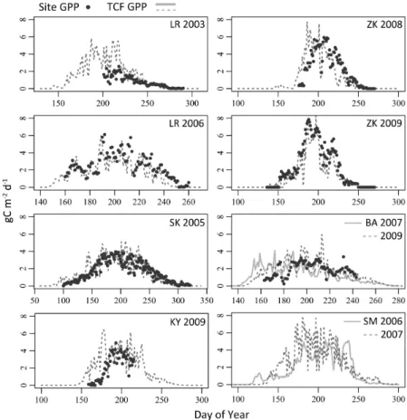
3.2 LUE based GPP

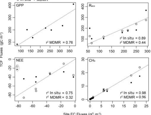
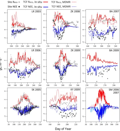
The TCF LUE model GPP simulations derived using MODIS and MERRA inputs cap-tured the overall seasonality observed in the tower EC records (Fig. 2) and explained 76 % (r2;p<0.05, N₌7) of variability in the total EC period-of-record fluxes (Fig. 3). While correspondence between the tower EC and TCF GPP estimates was also strong 5

(r2=75±16 %) for the 8 day cumulative fluxes, model-tower agreement decreased considerably for daily GPP (r2=57±22 %). The lower daily correspondence partially

reflects a delayed response in vegetation productivity and growth following changes in atmospheric and soil conditions (Lund et al., 2010) that was not adequately rep-resented in the LUE model. Temporal fluctuations in MERRA SW_rad also contributed 10

to short-term increases in TCF simulated GPP that were not always observed in the tower EC records. In addition, an insuﬃcient representation of seasonal phenology by the TCF LUE model may have contributed to diﬀerences between the tower and TCF GPP fluxes. This was most apparent for the Barrow and Kytalyk sites where the TCF re-sults overestimated the tower GPP fluxes towards the start of growing season (Fig. 2). 15

The large increase in TCF GPP at Kytalyk from 8–30 June (DOY 159–181) resulted from a short-term warming event observed in both the MERRA reanalysis and local tower temperature measurements that was not reflected in the EC GPP estimates. To examine the possibility that a shallow (<14 cm) early season thaw depth within the Ky-talyk tower footprint may have reduced the degree of vegetation response to short-term 20

warming, particularly for deeper rootingBetula nana and Salix pulchra, an additional simulation was conducted using the temperature driven bud break phenology model described in Parmentier et al. (2011a) to determine the start of LUE derived GPP ac-tivity. This step reduced the corresponding TCF and tower GPP RMSE diﬀerence for Kytalyk by 56 %, from 2.2 to approximately 1 g C m−2d−1with an associatedr2of 67 %. 25

(23)

BGD

10, 16491–16549, 2013

J. D. Watts et al.

Title Page

Tables Figures

◭ ◮

Back Close

Full Screen / Esc

Discussion

P

a

per

|

D

iscussion

P

a

per

|

Discussion

P

a

per

|

Discuss

ion

P

a

per

|

bryophyte sensitivity to surface drying (Wu et al., 2013). The additionalθconstraint re-duced the overall TCF and tower GPP RMSE (1.3 vs. 1.5 g C m−2d−1) and MRE (−0.1 vs. −0.8 g C m−2d−1) diﬀerences by approximately 14 and 92 %. However, the TCF simulations continued to overestimate the EC based GPP fluxes for Siikaneva, Lena River in 2003, and Kytalyk (MRE=−0.6±0.8 g C m−2d−1), and slightly underestimated 5

GPP elsewhere (MRE=0.3±0.3 g C m−2d−1). This variability in model GPP bias could be influenced by inconsistencies between the coarse scale MERRA inputs and local tower meteorology, which have also been reported elsewhere (i.e. Yi et al., 2013). For instance, periods of warmer (3 to 4◦C) MERRATmin inputs relative to local

measure-ments for the Lena River site in 2003 resulted in seasonally higher model GPP fluxes. 10

In contrast, mid-summer MERRAT_minfor the Barrow northern tower site in 2007 was 2 to 7◦C cooler than the local tower meteorology and led to significantly lower (p<0.05) model GPP estimates. Some of the observed biases between the TCF derived and site GPP estimates could also be due to site-specific di_ﬀerences in the light response curve and respiration model parameterizations (i.e. Aurela et al., 2007; Kutzbach et al., 15

2007; Parmentier et al., 2011a; Tagesson et al., 2012; Zona et al., 2012) used when partitioning the EC NEE fluxes into GPP andR_eco. However, it is di_ﬃcult to quantify the extent to which discrepancies between the TCF and EC derived GPP estimates can be directly attributed to the flux partitioning routines.

3.3 Recoand NEE 20

The TCF model R_eco simulations derived using local tower inputs accounted for 59±28 % and 76±24 % (r2) of variability in respective daily and 8 day cumulative tower EC fluxes (Fig. 4). As observed with GPP, the correspondence between the in-situ TCF modelR_eco results and tower EC records increased to 89 % (r2;p<0.05,N=6) when considering total-period cumulative fluxes (Fig. 3). The RMSE diﬀerences between the 25

in-situ TCFRecoand tower EC records varied considerably (0.3 to 1.3 g C m

−2

(24)

BGD

10, 16491–16549, 2013

J. D. Watts et al.

Title Page

Tables Figures

◭ ◮

Back Close

Full Screen / Esc

Discussion

P

a

per

|

D

iscussion

P

a

per

|

Discussion

P

a

per

|

Discuss

ion

P

a

per

|

for the Siikaneva, Lena River (2006) and Zackenberg sites and overestimated tower

Reco (−1≤MRE≤ −0.1 g C m

−2

d−1) elsewhere. Additional TCF simulations were con-ducted for selected tower sites having 10 cm depthTsrecords to examine the potential

influences of colder sub-surfaceT_s conditions on modelR_eco activity that were not ac-counted for by the shallow (≤5 cm in-situ depth) temperature inputs (Parmentier et al., 5

2011a). These simulations reduced overall RMSE diﬀerences between the in-situ TCF and towerR_eco estimates (reported in Table 2) by approximately 12 %. The TCF NEE estimates derived from local tower observations explained approximately 75±12 % and 81±11 % (r2) of respective daily and 8 day cumulative variability in the tower EC records (Table 2). Ther2correspondence between the in-situ TCF model NEE and total 10

period-of-record tower fluxes was also 75 % (p≤0.05) when excluding the Kytalyk site,

for which the TCF estimates were exceptionally low relative to the EC observed NEE sink (−16.3 vs. −81.8 g Cm−2). The overall RMSE and MRE diﬀerences between the

in-situ TCF and tower NEE records were 0.7±0.4 g C m−2d−1and 0.1±0.4 g C m−2d−1

respectively. 15

The TCFReco results derived using coarser MODIS and MERRA inputs accounted

for 51±29 % and 71±17 % (r2) of variability in respective daily and 8 day tower EC

records (Fig. 4; Table 2). However, only 44 % of the variability in the total period-of-recordReco fluxes was explained by the MODIS and MERRA based TCF simulations

(Fig. 3) due to higher (by approximately 170 %) modelR_eco predictions for Kytalyk and 20

Lena River (2003). The RMSE and MRE diﬀerences between the MODIS and MERRA driven TCF and tower Reco estimates were 0.9±0.4 and −0.2±0.9 g C m

−2

d−1, re-spectively. Using the internal TCF model GPP estimates increased the overall model and tower RMSE diﬀerences forReco by 23 % relative to the in-situ TCF results,

com-pared to a respective 3 and 14 % increase when incorporating MERRAθorTs inputs

25

(Fig. 5). Tower and TCF correspondence forR_ecoat the respective daily and 8 day time steps was also lower (r2=32 % and 56 %) for simulations using the internal TCF GPP estimates, relative to those derived using MERRAθorTsinputs (r

2

(25)

BGD

10, 16491–16549, 2013

J. D. Watts et al.

Title Page

Tables Figures

◭ ◮

Back Close

Full Screen / Esc

Discussion

P

a

per

|

D

iscussion

P

a

per

|

Discussion

P

a

per

|

Discuss

ion

P

a

per

|

The model and tower NEE correspondence derived using the MODIS and MERRA TCF inputs was strong at the 8 day time step (r2≥85 %) for Siikaneva, Lena River (2003) and Zackenberg (2009) compared to lower correspondence (r2≤45 %) for the other site records (Table 2). The relationship between the tower NEE records and MODIS and MERRA based TCF results was not significant for Kytalyk and the north-5

ern Barrow site in 2007 (r≤0.20;p≥0.16). Overall, the TCF NEE results derived using MERRAθandT_sinputs explained approximately 56 % and 72 % (r2) of the respective daily and 8 day cumulative variability in the tower EC fluxes (Fig. 5). This decreased to 32 % (daily) and 56 % (8 day cumulative), respectively, when substituting the internal TCF LUE estimates for the input tower GPP records. Similar decreases in temporal 10

correspondence between model derived carbon fluxes and wetland EC observations have been reported elsewhere (Zhang et al., 2012b) and are often influenced by tem-poral lags between fluctuating environmental conditions and carbon emissions (Levy et al., 2012). The RMSE di_ﬀerence between the MODIS and MERRA TCF based NEE simulations and the tower EC records averaged 1 (±0.5) g C m−2d−1, which is similar 15

to the results from previous TCF based studies using coarse resolution satellite remote sensing and reanalysis information (Yi et al., 2013). As observed with the in-situ based TCF model results, the largest diﬀerence in total record-period NEE occurred for Ky-talyk where the MODIS and MERRA based TCF simulations indicated only a small net carbon gain (−24.7 g C m−2) relative to the tower EC record (−82.4 g C m−2; Fig. 3). An

20

overall positive bias in the TCF model NEE fluxes (MRE=0.3±0.5 g C m−2d−1) was observed in the MODIS and MERRA TCF based simulation results (Table 2), but de-creased to 0.1±0.2 g C m−2d−1when excluding the less favorable Kytalyk and Barrow

northern record estimates (MRE≥0.9 g C m−2d−1).

3.4 CH4fluxes 25

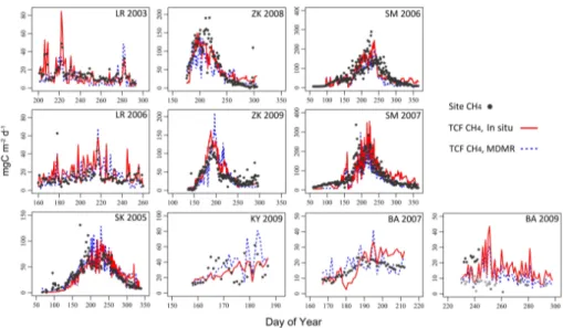
The TCF model CH4 simulations derived using local tower inputs accounted for

64±11 % (excluding Kytalyk;p=0.10) and 80±12 % (r2) of respective variability in the

(26)

es-BGD

10, 16491–16549, 2013

J. D. Watts et al.

Title Page

Tables Figures

◭ ◮

Back Close

Full Screen / Esc

Discussion

P

a

per

|

D

iscussion

P

a

per

|

Discussion

P

a

per

|

Discuss

ion

P

a

per

|

timates for these sites that were obtained using more complex biogeochemical models (e.g. Wania et al., 2010; Zhang et al., 2012b; Zürcher et al., 2013). Ther2 correspon-dence between the in-situ TCF simulations and tower CH4 fluxes increased to 98 %

when considering total period-of-record emissions across all sites (Fig. 3; p<0.05,

N=9). For the Kytalyk site, Parmentier et al. (2011b) reported large diﬀerences in EC 5

half-hourly CH4fluxes due to short term changes in wind direction. Larger CH4

emis-sions were often observed when the EC fluxes represented upwind portions of the tower footprint containing inundated microsites or plant communities such asCarexsp. andE. angustifolium. Although this short-term variability in CH4 fluxes may have

con-tributed to the observed discrepancy between the TCF and EC based emission esti-10

mates, attempts to systematically screen the EC observations based on wind direction, or to use daily EC medians instead of mean values, did not substantially improve the model results.

The RMSE di_ﬀerences between the local TCF CH₄ fluxes and tower records varied from 6.7 to 42.5 mg C m−2d−1. The local TCF simulations over predicted the EC tower 15

CH4 fluxes (−12.6≤MRE ≤ −1.2 mgC m

−2

d−1) for the Siikaneva, Lena River 2006, Zackenberg 2009, and Barrow 2009 north and central tower records, and underesti-mated tower CH4 fluxes (0.5≤MRE≤6.3 mg C m

−2

d−1) elsewhere. Incorporating µm

as an additional TCF CH4model constraint better elucidated the temporal variability in

CH₄emissions influenced by localized changes in gas flow between vegetation and the 20

atmosphere (Grosse et al., 1996; Joabsson et al., 1999). Without includingµm in the

model, the mean daily correspondence between the tower EC and TCF CH4fluxes

de-creased tor2<40 % and RMSE increased by>10 %. The most substantial diﬀerence in the TCF model results was observed for Lena River, where excluding theµmmodifier

reduced the daily and 8 day emissions correspondence by over 60 %. Theµmmodifier

25