Abstract
This article presents the results of numerical investigation on modeling buckling behavior and ultimate strength of corroded multi-planar tubular joints. Finite element method was used in order to simulate the behavior of DX multi-planar tubular joints under axial compressive loading.
Three different patterns were chosen for corrosion modeling. Also the effects of corrosion-related parameters such as age and depth of corrosion were evaluated. The first corrosion pattern is based on uniform reduction of wall thickness over a portion of tube length while the second pattern represents a sinusoidal reduction of thickness. The third pattern of corrosion uses average thickness and standard deviation as main parameters for defining a random corroded region. A linear criterion for predicting corrosion wastage has been used for the first and the second patterns, whereas pre-dictions of the third pattern are determined by a nonlinear meth-od.
The results indicate differences in the ultimate strength concluded from different patterns. It was found that conventional methods are conservative in evaluating the strength of corroded tubular joints of jacket platforms. Amongst 3 methods used for modeling corrosion, the third and the second pattern had similar results. It was also shown that corrosion is ineffective in braces and increas-ing the number of waves for the second pattern will result in in-crease of joint strength.
The optimum sizes of elements were defined by implementing an analysis of model sensitivity toward element size.
Keywords
Multi-planar tubular joints, DX joints, corrosion, Finite Element Method (FEM), ultimate strength, jacket platform.
Numerical Modeling of Corrosion Effectson
Ultimate Strength of DX Tubular Joints
Majid Rashidi a Masoud Nazari a
Mohammad Reza Khedmati a,* Akbar Esfandiari a
a Department of Maritime Engineering,
Amirkabir University of Technology, 424 Hafez Avenue, Tehran 15916-34311, Iran
*Author email: [email protected]
http://dx.doi.org/10.1590/1679-78253118
1 INTRODUCTION
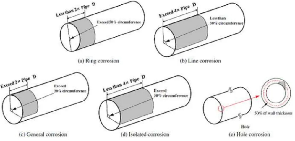
Introduction of modern methods for petroleum extraction and economic benefits of using old plat-forms result in utilizing platplat-forms beyond their design service lives. Therefore, for the purpose of safety and maintenance of a platform, it is necessary to investigate the remaining strength of cor-roded joints. Corrosion is a time-dependent electrochemical process and depends on the circum-stances surrounding the structure. It should be noted that corrosion is occurs in the form of galvanic type in the sea environment (Cosham et al. (2007)). Corrosion is usually divided into two main groups: general and localized corrosion. In case of tubular members, especially in the sea, the defini-tion is different. According to Hairil Mohd and Paik (2013), the corrosion definidefini-tion in terms of the extent of the corrode area is divided into 5 groups of ring, line, general, limited and hole corrosion. Each corrosion type affects a specific area of the tube. The dimensions of damaged area can be ex-pressed by multiples of tube diameter (D) in circumferential and longitudinal direction of the tube. Figure 1 shows corroded area dimensions for 5 corrosion types.
Figure 1: Different corrosion types and development of damaged area over the surface of tubular members (Hairil Mohd and Paik (2013)).
There are many factors affecting the speed of corrosion propagation, e.g. polarity of the metal, temperature, water flow rate, pH of sea water and the location of structure (Chamberlain (1988) and Wika (2012)).There is not a comprehensive research performed on ultimate strength of corroded joints and in general it is suggested that the designer should consider 10-12 mm (if no anti-corrosion coating is included) to compensate reduction of corrosion thickness for tubular members (UEG off-shore Research (1985).In jacket platform, tubular joints play an important role in load bearing and structural strength. As important structural elements, the study of static strength gives an overall prospect of entire structure.
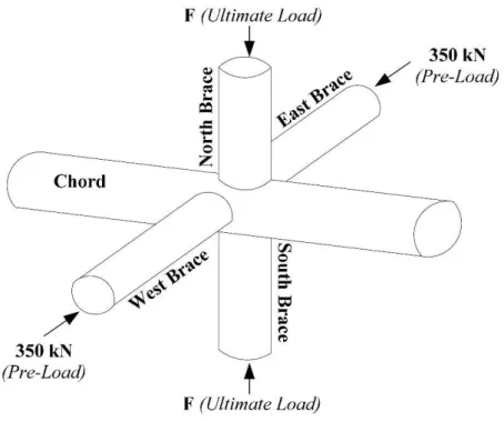
Numerical models and empirical formulas were used in these issues for different joints. Re-searches in the field of tubular joints can be categorized into three main groups, i.e. experimental, numerical and analytical studies. Empirical studies began in the 60s by Togo et al. (1967) and Washio et al.(1968-69). Among the most important researches, Chiew et al. (1997) performed a test on a DX joint to obtain its ultimate strength (Figure 2). The test conditions were similar to the real conditions and a full scale model was used. In this test the ultimate static strength of the joint was studied under compressive loading of bracing members, so that 350 kN was first applied to the out of plane braces and then 400 kN was applied to the in-plane braces. Afterwards the loading was only applied to in-plane braces and increased in controlled manner until the plastic deformation of the chord occurred.
Figure 2: 3 steps of loading for a DX joint (Chiew et al. (1997)).
shear are used to determine tubular joint strength. Marshall et al. (1974) investigated joint strength using punching shear model. Lan et al. (2016) studied on internally ring-stiffened tubular DT-joints to obtain static strength formula and comparing them with numerical models.
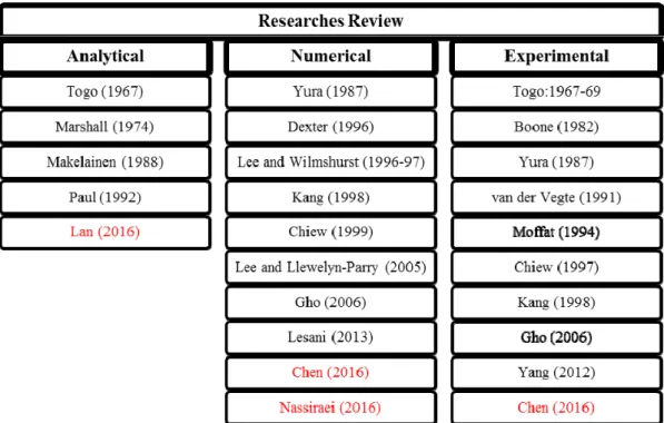
A summary of researches in three groups of experimental, analytical and numerical studies for a variety of joints is depicted in Figure 3. As mentioned earlier, there is no investigation performed on the ultimate strength of joints with corrosion. Extensive researches have been carried out on strengthening of intact tubular joints; but there is a lack of knowledge on prediction of strength for aged structures. The reason is difficulties of analyzing corroded joint, especially for large experi-mental scales. Furthermore, complexities and novelties of corrosion modeling make it to be an un-touched field of research.
In this paper a numerical method is used in order to determine the ultimate static strength of corrode DX joints. To do this, bracing member is loaded until the displacement-force curve reaches a maximum point (ultimate state).The validation of numerical model for non-corroded models is demonstrated for different kinds of loading conditions and boundary conditions.
The aims of this study can be listed as:
1.Modeling the thickness changes of the joint members using an efficient method that can effec-tively represent environmental conditions of the sea.
2.Obtaining the ultimate static strength of the corroded joint
3.Comparing the ultimate strength of the corroded joint with the intact joint. 4.Investigating the effects of basic parameters of corrosion patterns.
5.Predicting the ultimate strength of corroded joints as a function of time.
2 FINITE ELEMENT ANALYSIS
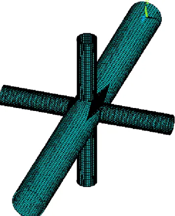
Due to complexities of stress distribution and load transmission mechanism for tubular joints, nu-merical methods are usually used to study behavior of tubular joints under different kinds of load-ing. In this study ANSYS 14 is used to conduct FE approach. The large deformation effects of nu-merical models involve nonlinearities of material and geometry. The material used has bilinear iso-tropic hardening properties. Accordingly, Von Mises yield criterion is introduced to Shell 181 ele-ments. Figure 4 shows an FE model of a DX joint used in this study.
Figure 4: An isometric view of a FE model for DX joint
2.1 Joint Model
are taken from Chiew et al. It should be noted that some joints with different geometrical proper-ties have been modeled but due to writing restrictions they were not mentioned in this paper. The total number of models was 75, and only 20 models are discussed in thisstudy.
2.2 Boundary Conditions and Principles of Modeling
The boundary conditions used for models were same as the experiments. For one-step and 3-step loadings, according to the different laboratory conditions and type of materials, two different meth-ods were used in applying boundary conditions.
2.2.1 One-Steploading
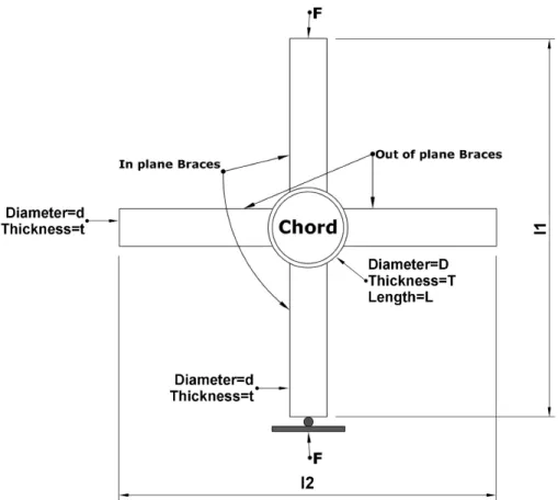
In this study the results of one step loading experiments performed by van der Vegte et al. (1991)are used. In other words, compression loading is applied to in-plane braces until the ultimate static strength is reached (Figure 5). According to Yura and Swenssen (1987), displacement control loading has been used.
Figure 5: Loading condition in one-step loading test (van der Vegte et al. (1991)).
L(mm) l1(mm)
l2(mm) D(mm)
d(mm) T(mm)
t(mm)
y
σ (N/mm^2)
2440 2856.4
2856.4 406.4
244.5 10
10 0.6 1 20 240
0.3
Table 1: Geometrical and mechanical properties of the DX-joint for one-step loading test (van der Vegte et al. (1991)).
Where:
d=The outer diameter of the brace member,
D=The outer diameter of the main member (chord) L=Length of the main member
t=Thickness of brace members T= Thickness of main member
l1=Length of in-plane braces including the outer diameter of the main member l2=Length of out of plane braces including the outer diameter of the main member
d =
D=Diameter ratio (indicating the density of the joint) t
T
= =Wall thickness ratio (indicating that the main member fails before the braces)
D 2T
= =Main member thickness parameter (indicating radial thickness and hardness of main
member)
y=Yield stress of steel
=Poisson's ratio
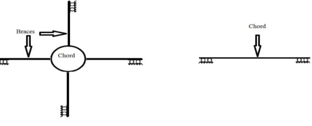
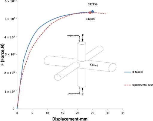
In this model, boundary conditions have been applied at the end of each member. In other words, 6 degrees of freedom for the elements at the end of members were constrained; only one axial translational degree of freedom is not fixed along of the member (Figure 6). The load-displacement curve for an experiment and the present FE model is shown in Figure 7.
Figure 7: Finite element modeling result for one-step loading test (ultímate strength) (van der Vegte et al. (1991)).
2.2.2 3-Step Loading
The 3-step loading was used for analyzing corroded models. According to researches conducted, loading on bracings, ≥12 coefficient(ratio of length multiplied by two to diameter of the main member) and support position of main member have no significant influence on the joint strength (Chiew et al. (1997)). This condition is the same as all corroded models. The procedure of loading is comprised of 3 different steps, i.e. at the first step, 350 kN compressive force is applied to the out of plane braces, then a force of 400 kN is applied to in-plane braces. Loading could change based on the joint capacity. Finally, a displacement controlled loading is applied on the joint until it fails (Chiew et al. (1997)). As previously mentioned, in these models bilinear isotopic hardening proper-ties have been used. As seen in Figure 8, the material reaches the yield strength with a fixed slope (Young's modulus E). After yielding, plastic behavior is expressed by another slope, say E1. Ac-cording to Khedmati research (2000), good value for E1 is E/65.
Figure 8: Stress-strain curve for 3-step loading.
L(mm) l1(mm)
l2(mm) D(mm)
d(mm) T(mm)
t(mm)
y
σ (N/mm2)
4997.2 2951.2
3079.2 457.2
273.05 9.3
9.1 0.6 0.98 24.5 361.8
0.3
Table 2: Geometrical and mechanical properties of DX-joint in 3-steps loading test (Chiew et al. (1997)).
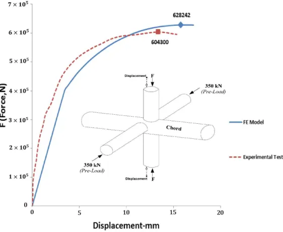
The boundary conditions are the same as one step loading models with the exception that from 6 degrees of freedom only 2 degrees of freedom for lateral translational is fixed (Figure 9). Figure 10 depicts the curves of load-displacement for an experiment and the present FE model. The ultimate strength obtained by numerical model differs from experimental results by about 3.9%. Also, the numerical force-displacement graph matches well with the experiment curve. The results of these two models (one-step and 3-step) indicate that the numerical models of DX tubular joints used in this study are reliable.
Figure 10: Finite element modeling result for 3-step loading test (ultímate strength) (Chiew et al. (1997)).
2.2.3 Corrosion modeling assumptions
As mentioned, there are different parameters for determining properties of a corroded region. In this study it is focused on two major parameters which are maximum depth of corrosion and corrosion distribution. The corrosion distribution is based on the average depth with standard deviation.
The data corresponding to these factors have been extracted and collected from sea filed. In or-der to study the effects of these two factors, three corrosion patterns have been used. The patterns are described in the following.
It should be noted that the starting time of corrosion is of important issue. It is assumed that corrosion begins in a range between 1.5 to 10 years after exposure to sea environment. According to research conducted by Guedes Soares and Garbatov (1999), corrosion starts a few years after the installation of structures in the environment and before that there is no significant corrosion (Emi et al. (1993), Loseth et al. (1994) and Guedes Soares and Garbatov (1999)). In this study, this time has not been considered wherever the age issue has been raised.
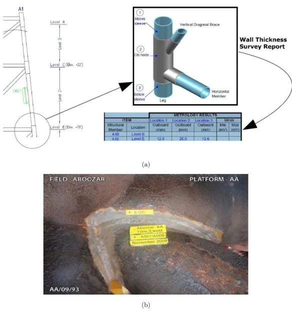
(a)
(b)
Figure 11: a) Routine inspection report of a platform in Persian Gulf b) A corroded member in Persian Gulf (Iranian Offshore Oil Company (2009)).
Time (Year) 5 25 50 75 100
max
Cr (mm) 0.55 1.90 3.75 5.60 7.50
Table 3: Maximum of corrosion depth (Crmax) (Houyoux and Alberts (2007)).
Where Crmaxis maximum corrosion depth andYearrepresents age of corrosion in years.
According to Melchers-South well nonlinear formula, based on the average depth with standard deviation (Qin and Cui (2003)), main parameters are as follows:
0.823 0.084
mean
Cr = Year (1)
0.823 0.056
SD
Cr = Year (2)
The average depth (Crmean) and standard deviation (CrSD) area function of structure age in
years.
2.2.4 Corrosion Applying
As mentioned above, corrosion can be categorized by its distribution on the surface of tubular members. In this study, two ways of applying general corrosion are used. Zone A and zone B repre-sents these two ways. Zone A is defined across the length of member, while zone B reprerepre-sents corro-sions with a length of more than twice the tube diameter and width of more than 30% of tube cir-cumference (Figure 1).
It should be noted that for some models, corrosion is only applied on the main member. On the other hand, in models with corrosion on braces, all of four braces have corrosion on their surfaces. Also in models with zone “B" which is assumed as locally corroded region, this area has been chosen on the main member at the vicinity of the joint. This is because of stress concentration in this re-gion and also the highest possibility of corrosion in the area. Figure 12 shows these two zones.
2.2.5 Corrosion Modeling Methods
In this study three methods of corrosion have been utilized. The characteristics of these models are based on maximum depth of corrosion and average corrosion depth with standard deviation.
2.2.5.1 First Corrosion Modeling Method
(a) (b)
Figure 12: a) Applied corrosion zone "A" b) Applied corrosion zone "B".
Figure 13: FE model of first corrosion modeling method applied on zone "B" forchord.
2.2.5.2 Second Corrosion Modeling Method
( )
11 0 , 1
max
Cr
t q t q p q p
p
= - - £ £ (3)
Figure 14: The cross section of a corroded tubular member with second corrosion pattern (one sided asymmetric external corrosión, Lutes et al. (2001)).
In this equation,t
( )
q1 is the thickness of the section of the member at angle 1q , and t0 is the initial thickness of the tube. Also, thickness changes in the longitudinal direction of the member. Figure 15 shows cross sections of tube at different locations. As Figure 15 shows, the ratio of thick-ness change shows a sinusoidal pattern both in circumferential and longitudinal direction. As shown in Figure 15, two equally sized waves are formed along the corrode region. Figure 16 shows how the number of waves changes in a fixed-length. Figures 17 and 18 show numerical models with this type of corrosion.
(a)
(b)
Figure 16: a) Schematic view of a corroded tubular member. b) FE model with four waves in zone "B" (Lutes et al. (2001)).
Figure 18: FE modelwithone wave in zone "A" forchord (second corrosion type).
2.2.5.3 Third Corrosion Modeling Method
This model is based on the average depth with standard deviation obtained from Melchers-South well formula by Melchers (1999) with a normal distribution (Wika (2012)). This model was only used for comparison with previous models. This model requires high density of meshing that in-creases the numbers of calculations. Therefore, only zone "B" in chord has finer mesh and corrosion applied in the same zone. Figure 19 shows a numerical mode of this type of corrosion.
Figure 19: FE model of corrosión for zone "B" onchord surface (third corrosion type).
2.2.6 Meshing
in the convergence of the finite element solution. The sensitivity of analysis toward the size of ele-ments was performed both for corroded and intact models. A numerical model for instance is com-prised of 17000 elements.
2.2.6.1 Appropriate Meshing Density for Corrosion Modeling
The sensitivity analyses led to choose a meshing with maximum element size of 4 cm. In order to precisely model a corroded plate, it is necessary to use much smaller elements, i.e. 1 mm (Rahbar-Ranji (2012)). Of course for plates, the plate dimensions are not as large as a tubular joint and the type of corrosion modeling usually differs from the tubes. For modeling corrosion of tubes, elements with 2 mm dimension have been used (Yamane (2006)). But Saad-Eldeen et al. (2013) used ele-ments of 5 cm dimension. Their study is close to this study in respect of structural aspects. Moreo-ver, a sensitivity analysis was performed on a joint with Chiew et al. (1997) geometry tests in the zone "B". Then in the same zone, second corrosion modeling method was applied and the same analysis was performed. In two models, at the zone "B" and for the main member, the element dimensions have been reduced from 40 mm to 9 mm. As dimensions of elements decrease, the vol-ume of nvol-umerical model and its processing time increase. The results of analyses are shown in figure 20.
In corroded model, the second type of corrosion was applied with one wave. Analysis was con-ducted with 40 mm elements and with the same corrosion at zone "B" with elements of 13 mm size.
Models with elements of 13 mm and 9 mm sizes showed no significant difference. As shown in Figure 20, these dimension changes have no clear change either with or without corrosion; therefore, 40 mm is a suitable dimension for elements.
3 RESULTS
In order to study the effects of geometry on strength of corroded joints, three different DX joints are modeled. The mechanical properties of these models are taken as same as joints of Chiew et al. (1997).Also the geometry of the models is equal to the experiments, e.g. the value of ratio is select-ed in such a way to minimize the effects of boundary conditions on joint behavior. Table 4 presents dimensions of DX joints.
Then based on the corrosion modeling methods discussed earlier, joints with corrosion were modeled. The characteristics of corrosion are presented in Table 5. As mentioned earlier, in order to study effects of different parameters 75 models were analyzed in this study. These parameters in-clude geometric, material properties and corrosion characteristics. Since the scope of this paper is to focus on effects of corrosion, the other models are not included. Also in order to emphasize the aims of the paper, the authors preferred to choose only 20 models. The ultimate strength of corroded models are compared with non-corroded models, i.e. Chiew et al. (1997) loading condition.
The ultimate strength of models are shown in tables 6. FCor indicates ultimate strength of the
joint with corrosion. If FCor=0 is right, it means that there is no corrosion on the joint and dFE
(a)
(b)
JointName D(mm) d(mm) L(mm) T(mm) t(mm) θ l2(mm) l1(mm)
DX6 500 300 5465 12 5 90 3122 2994 0.600 0.416 20.83 DX9 500 300 5465 12 10 90 3122 2994 0.600 0.833 20.83
DX10 500 300 5465 12 12 90 3122 2994 0.600 1 20.83
Table 4: Dimensions of joints DX6, DX9 and DX10.
De sc ri pti on Corrosion Properties (mm) Corrosion in Braces Corrosion in Chord
Age of Corrosion (Year)
Preloading (k N) Purpose Geometr ica l Pr operties Mode l N umbe r Mode l Zone Mode l Zone
With One Wave 1.9
2nd B 25
320
Wave Num. Ef
fect in 2
nd co
rr osión modeling meth od DX9 59 With Two Waves 1.9 2nd B 25 DX9 60 With Four Waves 1.9 2nd B 25 DX9 61
With One Wave 1.9 2nd A 2nd A 25 320
Effect of Co
rro
sion in Braces
DX6 21
With One Wave 1.9 2nd A 2nd A 25 DX10 25 1.9 1st A 1st A 25 DX6 36 1.9 1st A 1st A 25 DX10 40
With One Wave 1.9 2nd A 25 DX6 66
(continuation) De sc ri pti on Corrosion Properties (mm) Corrosion in Braces Corrosion in Chord
Age of Corrosion (Year)
Preloading (k N) Purpose Geometr ica l Pr operties Mode l N umbe r CrSD Crmean Crmax Mode l Zone Mode l Zone 1.9 1st A 25 320
Effect of Co
rro
sion in Braces
DX6 67 With One Wave 1.9 2nd A 25 DX10 68 1.9 1st A 25 DX10 69 1.9 1st B 25 320 Comparing 3 rd corros
ion modeling m
ethod with 1
st & 2
nd DX10 70 With One Wave 1.9 2nd B 25 DX10 71 0.792 1.188 3nd B 25 DX10 72 0.55 1st B 5 DX10 73 With One Wave 0.55 2nd B 5 DX10 74 0.211 0.3158 3nd B 5 DX10 75
Figure 21: Stress distribution and deformation of DX6 joint at the ultimate strength state. FE d (mm) 0 Cor F = Or Cor F (kN) Model Number FE d (mm) 0 Cor F = Or Cor F (kN) Model Number 17 817.8579 66 17 920.6976 6 17 710.4593 67 18 935.2138 9 17 800.5501 68 18 925.3163 10 18 712.7219 69 15 837.4587 59 16 755.7378 70 16 847.6352 60 15 832.8621 71 16 861.2652 61 16 828.3735 72 17 817.884 21 15 867.2978 73 16 799.9786 25 15 896.9807 74 18 691.4704 36 15 882.5071 75 17 711.1212 40
The models 6, 9 and 10 are intact joints and have no corrosion. The reduction of ultimate strength for the remaining 17 models can be obtained using table 6.
The first pattern is a common way of modeling corrosion defects. Joints with this kind of corro-sion demonstrate the lowest level of strength. e.g. the strength of models 36 and 40 is reduced by 25% and 23.2% respectively; while for the joints with the same conditions, but with the second cor-rosion pattern, i.e. models 21 and 25, reductions of 11.2% and 13.5% are observed.
The joints 59, 60 and 61 have corrosion defects based on the second pattern. As it is presented in table 6, an increase in the number of waves from 1 to 4, causes a reduction of about 2.5% in ul-timate strength.
Also, the strength of a corroded joint depends on location of damaged area. As it is shown in the table 6, one can say that tubular DX joints with the first and second patterns of corrosion show similar behaviors in relation to location of damaged area. According to models 68 to 71, it is found that for the first pattern, 6% of strength drop occurs for the joint with corrosion at zone A com-pared to the joint with corrosion at zone B. This difference is expected to be 4% for the second pattern corrosion. In the next sections, these strength reductions discussed.
3.1 Effect of Number of Corrosion Waves
Figure 22 shows effect of number of corrosion waves on ultimate strength of DX joints. One can say that for joints with second corrosion pattern, as the number of waves increases, the ultimate strength of joints increases.
Figure 22: Effect of wave number on ultímate strength of joints with second corrosión pattern.
3.2 Behavior of Joints with Corroded Braces
Diffrence of Non-Corroded brace Model With Corroded One Diffrenc with Non-Corrode Model (%) Cor F (kN) Corrosion Zone Corrosion Model Geometrical Properties Mod- el-Number 2.67 22.83 710.4593 A (Non-Corroded Braces) 1st DX6 67 24.9 691.4704
A (Corroded Braces) 1st 36 0.003 11.17 817.8579 A (Non-Corroded Braces) 2nd 66 11.17 817.884
A (Corroded Braces) 2nd 21 0.22 23.22 712.7219 A (Non-Corroded Braces) 1st DX10 69 25.27 711.1212
A (Corroded Braces) 1st 40 0.07 11.61 800.5501 A (Non-Corroded Braces) 2nd 68 11.61 799.9786
A (Corroded Braces) 2nd
25
Table 7: Effect of corrosion in braces.
3.3 Comparison of the Three Corrosion Patterns
Table 8 shows that the third corrosion pattern matches well with the second pattern. This corrosion model is more detailed and adapted to reality. It is also comprised of more elements that causes a time consuming process. Therefore, the second model is a suitable corrosion pattern to be studied in this paper.
Diffrence of 3rd Model
With 2nd Model
(%) Diffrence of
3rd Model with 1st Model
(%) Cor F (kN) Corrosion Age (Year) Corrosion Model Geometrical Proper-ties Model Num-ber 0.54 8.77 755.7378 5 1st DX10 70 832.8621 5 2nd 71 828.3735 5 3rd 72 1.64 1.75 867.2978 25 1st DX10 73 896.9807 25 2nd 74 882.5071 25 3rd 75
4 CONCLUSIONS
A numerical study on ultimate strength of 20DX tubular joints with corrosion defects was conduct-ed. Three different corrosion patterns were discussed, and reduction of ultimate strength in terms of corrosion characteristics was presented. The effects of these three corrosion patterns were also com-pared with each other.
A sensitivity analysis was performed in order to achieve a balance between mesh sizing and ac-curacy of the results. The optimum element sizes were selected regarding dimensions of joint and corroded area.
The first corrosion pattern was modeled as a uniform reduction of wall thickness in a confined region. This pattern was based on linear relation of corrosion depth and time. Empirical equations were used to predict material loss in terms of time. Then the ultimate strength of the joints was obtained as a function of structure age. Due to higher material loss, joints with the first corrosion pattern showed more reduction of ultimate strength than ones with the other two patterns. This implies that common ways of corrosion modeling are very conservative.
The non-uniform material loss of joints with the second pattern was modeled by sinusoidal forms over tubular surfaces. The relation between decrease in joint strength and number of sinusoi-dal waves of corrosion was studied. It was shown that an increase in the number of waves causes a reduction in effects of corrosion.
In order to predict corrosion characteristics of the third pattern, a nonlinear criterion was used. The average corrosion depth and standard deviation of thickness were chosen for random distribu-tion of thickness over the surfaces.
Also it was found that the effects of corrosion reduce in cases where corrosion occurs on brace surface. However, for joints with the first corrosion pattern, as the ratio of the maximum depth of corrosion to the initial thickness increases, braces become vulnerable to failure.
The importance of affected zone location was also investigated. The analyses demonstrated that thickness changes of the chord on the vicinity of joints play an important role on ultimate strength. In the other words, the surface of the chord member at the intersection of braces is of great signifi-cance and special attention should be paid for corrosion protection of this area.
References
ANSYS 14.0 reference manual (2012). ANSYS Inc.
Boone, T. J., Yura, J. A., Hoadley, P. W. (1982). Chord stress effects on the ultimate strength of tubular joints, P. M. Furguson Struct. Eng. Lab Rep. 82-1, Univ. of Texas at Austin, Austin, Tex., USA.
Chamberlain, J. (1988). Corrosion for students of science and engineering, Longman Scientific & Technical.
Chen, Y., Feng, R., Xiong, L. (2016). Experimental and numerical investigations on double-skin CHS tubular X-joints under axial compression. Thin-Walled Structures, 106: 268-283.
Chiew, S.P., Soh, C.K., Fung, T. C. (1997). Large Scale Testing of a Multiplanar Tubular DX-Joint. Proceedings of the Seventh International Offshore and Polar Engineering Conference Honolulu, USA.
Chiew, S.P., Soh, C.K., Fung, T.C., Soh, A.K. (1999). Numerical study of multiplanar tubular DX-joints subject to axial loads. Computers and Structures, 72: 749-61.
Dexter, E. M. (1996). Effects of overlap on behaviour and strength of steel circular hollow section joints, PhD thesis, University of Wales, Swansea, Wales.
Emi, H., Yuasa, M., Kumano, A., Arima, T., Yamamoto, N., Umino, M. (1993). A study on life assessment of ships and offshore structures (3rd report: corrosion control and condition evaluation for a long life service of the ship). J Soc Nav Archit Jpn, 174: 735-744.
Gho, W.M., Gao, F., Yang, Y. (2006). Strain and stress concentration of completely overlapped tubular CHS joints under basic loadings. Journal of Constructional Steel Research, 62: 656–674.
Gho, W.M., Yang, Y., Gao, F. (2006). Failure mechanisms of tubular CHS joints with complete overlap of braces. Thin-Walled Structures, 44: 655–666.
Guedes Soares, C., Garbatov, Y. (1999). Reliability of maintained, corrosion protected plates subjected to nonlinear corrosion and compressive loads. Marine Structures, 12: 425-445.
Hairil Mohd, M., Paik, J.K. (2013). Investigation of the corrosion progress characteristics of offshore subsea oil well tubes. Corrosion Science, 67: 130-141.
Houyoux, C., Alberts, D. (2007). Design method for steel structures in marine environment including the corrosion behavior (European Commission), Vol. 1, First Edition, RFCS publications.
Iranian Offshore Oil Company (2009). Final report jacket inspection (Aboozar Field), Report No: 09/11/245.
Kang, C. T., Moffat, D. G., Mistry, J. (1998). Strength of DT tubular joints with brace and chord compression. Journal of Structural Engineering, 124: 775-783.
Khedmati, M.R. (2000). Ultimate strength of ship structural members and systems considering local pressure loads, Dr Eng thesis, Graduate School of Engineering, Hiroshima University, Japan.
Lan, X., Wang, F., Ning, C., Xu, X., Pan, X., Luo, Z. (2016). Strength of internally ring-stiffened tubular DT-joints subjected to brace axial loading. Journal of Constructional Steel Research, 125: 88-94.
Lee, M. M. K., Llewelyn-Parry, A. (2005). Strength prediction for ring-stiffened DT-joints in offshore jacket struc-tures. Engineering Structures 27: 421–430.
Lee, M. M. K., Wilmshurst, S. R. (1996). A parametric study of strength of tubular multiplanar KK-joints. Journal of Structural Engineering, 122: 893–904.
Lee, M. M. K., Wilmshurst, S.R. (1997). Strength of multiplanar KK-joint under anti symmetrical loading. Journal of Structural Engineering, 123: 755–64.
Lesani, M., Bahaari, M. R., Shokrieh, M. M. (2013). Detail investigation on un-stiffened T/Y tubular joints behavior under axial compressive loads. Journal of Constructional Steel Research, 80: 91-99.
Loseth, R., Sekkeseter, G., Valsgard, S. (1994). Economics of high tensile steel in ship hulls. Marine Structures, 23: 31-50.
Lutes, L. D., Kohutek, T.L., Ellison, B.K., Konen, K.F. (2001). Assessing the compressive strength of corroded tubu-lar member. Applied Ocean Research, 23: 263-268.
Makelainen, P. K., Puthli, R. S. (1988). Semi-analytical models for the static behavior of T and DT Tubular joints. International Conference on Behaviour of Offshore Structures (BOSS), Trondheim, Norway, 1285-1300.
Marshall, P. W., Toprac, A. A. (1974). Basis for tubular joint design. Welding Journal, 53: 192-201.
Miki, C., Kobayashi, T., Oguchi, N., Uchida, T. (2000). Deformation and fracture properties of steel pipe bend with internal pressure subjected to in-plane bending, WCEE.
Moffat, D. G., Kruzelecki, J., Blachut, J. (1994). Static strength of T and DT tubular joints in offshore structures, Rep. No. A/169194, University of Liverpool, Liverpool, U.K.
Nassiraei, H., Lotfollahi-Yaghin, M. A., Ahmadi, H. (2016). Static strength of doubler plate reinforced tubular T/Y-joints subjected to brace compressive loading: Study of geometrical effects and parametric formulation. Thin-Walled Structures, 107: 231-247.
Paul, J. C. (1992). The ultimate behavior of multiplannar TT-and KK-Joints made of circular hollow sections, PhD thesis, Kumamoto University, Kumamoto, Japan.
Qin, S., Cui, W. (2003). Effect of corrosion models on the time-dependent reliability of steel plated elements. Marine Structures, 16:15-34.
Rahbar-Ranji, A. (2012). Ultimate strength of corroded steel plates with irregular surfaces under in-plane compres-sion. Ocean Eng., 54: 261-269.
Saad-Eldeen, S., Garbatov, Y., Guedes Soares, C. (2013). Ultimate strength assessment of corroded box girders. Ocean Eng, 58: 35-47.
Togo, T. (1967). Experimental study on mechanical behaviour of tubular joints, PhD dissertation, Osaka Univ., Osaka, Japan.
UEG offshore Research (1985). Design of tubular joints for offshore structures Vol.3, UEG offshore Research.
van der Vegte, G.J., de Koning, C.H.M., Puthli, R.S., Wardenier, J. (1991). The Static Strength and Stiffness of Multiplanar Tubular Steel X-Joint. International Journal of Offshore and Polar Engineering, 1: 42-52.
Washio, K., Togo, T., Matsui, Y. (1968). Experimental studies on local failure of chords in tubular truss joints: Part I, Technol. Rep., Osaka Univ., Osaka, Japan.
Washio, K., Togo, T., Matsui, Y. (1969). Experimental studies on local failure of chords in tubular truss joints: Part II., Technol. Rep., Osaka Univ., Osaka, Japan.
Wika, S.F. (2012). Pitting and Crevice Corrosion of Stainless Steel under Offshore Conditions, Msc Thesis, Norwe-gian University of Science and Technology, Trondheim, Norway.
Yamane, M. (2006). Residual Strength Evaluation of Corroded Steel Members in Marine Environments. Proceedings of the Sixteenth International Offshore and Polar Engineering Conference, 43-50.
Yang, J., Shao, Y., Chen, C. (2012). Static strength of chord reinforced tubular Y-joints under axial loading. Marine Structures, 29: 226-245.