Buckling Analysis of Laminated Anisotropic Kirchhoff’s Plates via The
Boundary Element Method
Abstract
A new fundamental solution for laminated anisotropic Kirchhoff’s plates with out-of-plane and in-plane compressive loads is derived here. The multicompressed solution for both isotropic and anisotropic cases is obtained via the Radon Transform. Some fundamental kernels of the integral equations are described in detail. BEM results of displacements and critical buckling loads of several plates with different boundary conditions and geometries are presented. Comparisons with available analytical solutions and some published numerical results confirm the reliability and accuracy of the proposed formulation.
Keywords
Fundamental solution, plates, anisotropy, laminated composites, buckling.
1 INTRODUCTION
Plates are important structural elements used in many engineering fields. For modern applications, such as in the aeronautical and automobile industries, there has been an increasing use of laminated anisotropic plates. Their usage in structural projects is highly advantageous since they are lighter and stronger than traditional materials like metals and metal alloys.
Many problems in anisotropic media cannot be solved analytically and so numerical methods are of paramount importance. The Boundary Element Method (BEM) is a well established alternative to the Finite Element Method (FEM). BEM discretizes the problem only on its boundary, which allows a reduction of the problem's dimension. When compared with FEM, BEM presents high precision on field variables.
Although BEM is highly efficient compared with FEM, it presents some difficulties such as the derivation of fundamental solutions and treatment of the domain integrals which appear e.g. when dealing with plate bending problems. On the other hand, unlike FEM, BEM does not suffer from numerical problems such as the shear locking when using the Shear Deformation Theory (SDT) of plates. Also BEM does not suffer from locking phenomenon due to high stiffness in preferred directions in anisotropic elasticity like FEM.
The bending problem of thin plates can be modelled by the Classical Plate Theory (CPT) (or Kirchhoff-Love theory) when the out-of-plane displacement is small and shear deformations are negligible. The first works using BEM to analyze the bending of thin plates with Kirchhoff-love's theory were presented in the 1970s. Some of those works can be found in Bézine (1978), Altiero and Sikarskie (1978), and Stern (1979). More recently, Dirgantara and Aliabadi (1999, 2006) investigated the bending and the large deflection of shells. Albuquerque et al. (2006) studied the bending of laminated composite Kirchhoff plates. Katsikadelis and Babouskos (2009) used BEM with the analog equation method to study bending and vibration of thick plates.
When there are compressive forces acting on the plate's midplane, an instability known as buckling may take place. Buckling may cause catastrophic failures to structures like plates. It is a highly non-linear phenomenon which is assessed with non-linear theories like the well known von Karman theory of plates. However, linearized theories
José I. L. Monteiroa* C. H. Darosb
aDepartamento de Mecânica Computacional, Faculdade de Engenharia Mecânica,
Universidade Estadual de Campinas - UNICAMP, Campinas, SP, Brasil. E-mail:
bDepartamento de Mecânica Computacional, Faculdade de Engenharia Mecânica,
Universidade Estadual de Campinas - UNICAMP, Campinas, SP, Brasil. E-mail:
* Corresponding author
http://dx.doi.org/10.1590/1679-78254341
are often used as means of obtaining critical loads for the pre-buckling stage. Such critical loads are extremely important as failure criteria for engineering applications. One of the first works applying BEM to plate buckling is Shi and Bézine (1990). Shi (1990) also studied the vibrational and buckling problem of thin plates with the direct boundary element method. Other works treating the buckling of plates and shells via the BEM can be seen in Syngellakis and Elzein (1994), and Baiz and Aliabadi (2007). Other numerical methods have been employed in the past for obtaining critical loads for plates within the realm of the linearized theory. For multi-compressed isotropic and/or anisotropic polygonal plates we may cite Liew and Wang (1995), Ferreira et al. (2011), and Shojaee et al.
(2012).
In this work we present numerical results for the problem of anisotropic Kirchhoff plates with the action of compressive and shear in-plane forces combined with an out-of-plane perturbation. The critical loads for several isotropic/anisotropic plates are obtained using a concentrated out-of-plane force. Hence, we avoid the use of domain integrals using a pure Boundary Element Method. For multi-compressed isotropic and anisotropic plates, new fundamental solutions are derived here via the Radon Transform. The results are compared with existing analytical or FEM results, showing an excellent agreement.
2 Governing equations
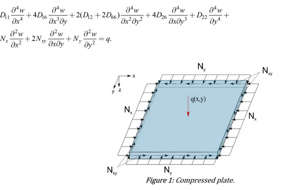
According to Kirchhoff's theory the transverse displacement w of multicompressed thin plates (Figure 1) can
be described by the following differential equation (see Lekhnitskii (1968) and Timoshenko and Woinowsky-Krieger (1959))
4 4 4 4 4
11 4 16 3 12 66 2 2 26 3 22 4
2 2 2
2 2
4 2( 2 ) 4
2 .
x xy y
w w w w w
D D D D D D
x x y x y x y y
w w w
N N N q
x y
x y
(1)
Figure 1: Compressed plate.
With Dij denoting the flexural rigidities. Since we shall focus on symmetric laminated anisotropic plates, the
final flexural rigidities can be obtained by adding the sequence of flexural rigidities of each rotated orthotropic ply.
3 3
1 1
1 ( ) (z z ). 3
l
ij ij k k k k
D Q
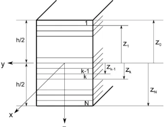
(2)With
z
k representing the distance from the middle plane to the ply's surfaces, k and k-1 (see Figure 2). (Qij k)is the reduced rotated matrix in the plane stress state with the elastic constants of each ply (Eq. (3)). In Eq. (2)
, 1,2,6
Figure 2: A symmetric laminated composite with N plies.
2 11 2 2 2 2 2 12 2 21 3 3 2 4 1
8 1
cos 2 cos 4
2 4 1 ,
2 1 8 1
1 6 4 1
8 1 cos 4
2 4
8 1
k k k k k k k
l t t lt lt lt
k lt
k k
k k k k k k k k
l t l t t lt lt lt
k k
lt lt
k k k k k k k
l t t lt lt lt
k lt k
k k k k
l t t lt
k lt
Q E E E G
E E E E E G
Q E E E G
E E E
2 216 2 2
2
22 2
2 2
1 ,
sin 2 sin 4
2 4 1 ,
4 1 8 1
1 3 3 2 4 1
8 1
cos 2 cos 4
2 4
2 1 8 1
k k
lt lt
k k
k k k k k k k k k
l t l t t lt lt lt
k k
lt lt
k k k k k k k
l t t lt lt lt
k lt
k k
k k k k k k k
l t l t t lt lt
k k
lt lt
G
Q E E E E E G
Q E E E G
E E E E E G
2 226 2 2
2
66 2
2 2
1 ,
sin 2 sin 4
2 4 1 ,
4 1 8 1
1 2 4 1
8 1 cos 4
2 4 1 .
8 1
k lt
k k
k k k k k k k k k
l t l t t lt lt lt
k k
lt lt
k k k k k k k
l t t lt lt lt
k lt k
k k k k k k
l t t lt lt lt
k lt
Q E E E E E G
Q E E E G
E E E G
(3)
3 Boundary Integral Equation
Using the weighted residual method in Eq. (1), we obtain the singular Boundary Integral Equation (BIE) for compressed anisotropic Kirchhoff's plates (see Albuquerque et al. (2006)),
* * * * 1 * * * 1 ( ) ( ) ( , ) ( ) ( , ) ( , ) ( ) ( ) ( , ) ( , ) ( ) ( ) ( , ) ( ) ( , ) . c j j c j j N
i i n i n i c i c n i
j N
i
n c c i i
j
w
c w V w d M d R w V w d
w
M d R w q w d
xx x x x x x n x x x x x x
x x
x n x x x x x x
(4)
With Γ and Ω representing the plate's boundary and domain, respectively; x x, i represent the field and source point, respectively; ci is a free term depending on the smoothness of the plate’s boundary; Mn represents the resultant moment (see Eq. (5)). Rcj is the corner reaction, described as
R
cjM
nsM
ns
; M n s are the twistingmoments after (+) and before (-) the corner (see Eq. (6)); wcjis the corner displacement and Nc is the total number
of corners. Vn represents here the resultant shear force for polygonal plates, which considers the effect of the out-of-plane and in-plane forces (see Eq. (8)). The starred terms are the known fundamental Kernels, which are obtained deriving the fundamental solution. *
n M , *
n s M , *
n Q , *
n
V are concisely expressed as
* 2 *
2
* 2 *.
n x x x y xy y y
M n M
n n M
n M
(5)
* * * 2 2 *
.
ns x y y x x y xy
M
n n M
M
n n M
(6)With
2 * 2 * 2 *
*
11 2 16 12 2
2 * 2 * 2 *
*
16 2 66 26 2
2 * 2 * 2 *
*
12 2 26 22 2
2 , 2 , 2 . x xy y
w w w
M D D x y D
x y
w w w
M D D x y D
x y
w w w
M D D x y D
x y (7)
With nx and ny denoting the direction cosines.
* * *
* * ns ,
n n M n w ns w
V Q s N n N s
(8)
3 * 3 * 3 * 3 *
*
11 3 16 2 12 66 2 16 3
3 * 3 * 3 * 3 *
16 3 12 66 2 26 2 22 3
3 2
2 3 ,
n x
y
w w w w
Q D D D D D n
x x y x y y
w w w w
D D D D D n
x x y x y y
(9)
2
2
2,
2 2.
n x x xy x y y y ns x y y x xy x y
N
N n
N n n N n
N
n n N
N
N n n
(10)∂/∂n and ∂/∂s are the derivatives in the normal and tangential directions, respectively, given by
nx n ,y ny n .x
x y x y
n s (11)
It is well known that due to the number of variables (Mn, Vn, w , w n/ ) a second equation is needed to fully
which present (1/r2) singularities. The latter require special analytical or numerical treatment since they are hypersingular in the sense of Hadamard.
*
* *
1 *
* 2 * *
1 ( , ) ( ) ( , ) ( ) ( , ) ( ) ( ) ( , ) ( , ) ( , ) ( , ) ( ) ( ) ( ) ( ) . c j j c j j N c i
i n i n i
i c
i i i j i
N c i
i i i
n n c
i i j i i
R
w V M w
c w d d w
w
w w w
V d M d R q d
x xx x x x x x x x
n n n n n
x x
x x x x x x
x n x n n x n x n
(12)
We used Eq. (12) for the isotropic case and hence we will present on following the detailed derivation of each Kernel for the singular and hypersingular BIEs. For the anisotropic case, due to the high complexity of the numerical integrations, we used the strategy of outside points of the boundary plate as in Paiva and Venturini (1992), hence using only the singular BIE. Moreover, for a concentrated out of plane load (Dirac's Delta load) the domain integrations disappear. It is then only necessary to evaluate the fundamental solution at the point of application as
*( ,i i)
w x x x .
4 Fundamental solution
4.1 Isotropic media
In this work, two fundamental solutions for isotropic plates are considered. One for the case with compressive forces only in one direction (unidirectionally compressed) and another for the case with the combined action of compressive forces in both direction with shear in-plane forces (multidirectionally compressed).
4.1.1 Unidirectionally compressed plates For this case, the governing equation is
2 4
2 . x w
D w N q
x
(13)
Jahanshahi and Dundurs (1964) constructed a solution for the problem of plates compressed in one direction and a moving out-of-plane load. Adapting their solution to the case of a fixed out-of-plane load, we have
| - | | - |
* 2 2
0 0
0 0
1 sin( )Y ( ) 1 (| - | )Y ( ) ,
8 8
i i
x x y y
i i
w D y y d D y y d
(14)Where ( , )x y and ( , )x yi i are the coordinates of the field and source points, respectively.
D
is the flexural rigidity, given by D Eh3/ (12(12)); Nx/ (4 )D ; Y0 and Y1 are the Bessel functions of the second kind of order0 and 1, respectively. Notice that w* and w*/n are not explicit, requiring further numerical integration. However, all other kernels are explicit. Deriving Eq. (14), we find
* 0 | - | * 0 0 | - | 2 2 1 2 2 0 2 *0 , 1
2 2 *
, 1
2 *
1 sin( ( ))Y ,
8
1 sign( ) Y ( )
8
1 ( ) sin( ) Y ( ( ) ) ,
8 ( )
1 cos( ( ))Y sin( ( ))Y ,
8
1 sin( ( ))Y ,
8 i i i y y i x x i i i
i x i
y i
w x x r
x D
w y y d
y D
y y y y d
D y y
w x x r r x x r
D x
w r x x r
x y D
w
0 , 1
2 81 cos( (D x xi))Y r rxsin( (x xi)) Y r .
y
With
r
(
x x
i) (
2
y y
i)
2, r,x (x x i) /r and r,y (y y i) /r. Using the following useful identity1 1
0
Y ( )r Y ( )r Y ( )r ,
r r
(16)
we may express the third order derivatives as
3 * 2, 0 , 1
3 2 ,
1 3 *
, , 0 , 1
2 , , 1 3 * 2 , 2
1 ( 2) sin( ( )) Y 2 cos( ( ))Y
8 1 2
sin( ( ))Y ,
1 sin( ( ))Y cos( ( ))Y
8 2
sin( ( )) Y ,
1 sin(
8
y i x i
y
i
x y i y i
x y
i
y
w r x x r r x x r
D x
r
x x r
r
w r r x x r r x x r
D x y
r r
x x r
r w r D x y
2 , 0 1 3 *, , 0 , 1
3
, ,
1
1 2
( ))Y sin( ( ))Y ,
1 sin( ( ))Y cos( ( ))Y
8 2
sin( ( ))Y .
y
i i
x y i y i
x y
i
r
x x r r x x r
w r r x x r r x x r
D y
r r
x x r
r (17)
Substituting the derivatives of Eq. (15) and Eq. (17) in Eqs. (5)-(11) we obtain the fundamental kernels of Eq. (4) and Eq. (12). For the sake of brevity we shall present here only one of the kernels, * /
n i
V
n which has been
derived, to the author's best knowledge, here for the first time.
* 2
1 0 2 1 3 0
2
4 1 5 2 1
cos (x x ) Y cos (x x ) Y sin (x x ) Y
1
sin (x x ) Y sin (x x ) Y .
n
i i i
i
i i
V D r D r D r
r r
D r D r
r
n (18)
Expressions for D1 to D5 can be found in Appendix A. The other kernels are presented in Monteiro Jr. and Daros (2017) and Monteiro Jr. (2017). For the sake of conciseness, we will only show here results for multidirectionally compressed plates.
4.1.2 Multidirectionally compressed plates The governing equation in this case is
2 2 2
4
2 2 2 .
x w xy w y w
D w N N x y N q
x y
(19)
We shall present here a new fundamental solution for this equation via the Radon Transform. The latter has been successfully used for several partial differential equations. For a complete review of the Radon Transform the reader is referred to Ludwig (1966) and Helgason (1980) where a thorough description of the Transform properties are given. The Radon Transform is defined as
ˆ
( ) ( , ) ( ) ( ) ( ) .
s
f f s
f dS
f s d x mm x x x m x
(20)
Where s x m is the transform hyperplane and m is the unit radius of the circle (Figure 3). Using the Radon
( , )
( ), ˆ ( ( ) ( )) ( ) kk ( , ).s
f f s
s
x ξ m ξ
x x m m
(21)Figure 3: Radon circle.
With ξ denoting the source point and ℒ represents here a linear partial differential operator. Applying the Radon Transform to Eq. (19), we find
2 ( 2 ) w (s, )* 1 (s ),
d s d s
D
m m ξ (22)
With
2 2
1 1 2 2
m 2 xym m ym .
x N N
N
D D D
(23)
With m1cos( ) and m2 sin( ) . Based on Manolis et al. (2003), we propose, for 0, Eq. (24) as a solution for Eq. (22),
* 1 i i |s |
w (s, ) 2D | s | e .
m ξ
m m ξ (24)
The inverse Radon transform is defined via the equation 1
2 | | 1
1 ( , )
ˆ
( ) ( ( , )) .
4 s
f p
f f s s d d
m m x
m
x m m (25)
Applying the Inverse Radon Transform in Eq. (24), we find
1
2 | | 1 i |s |
1
2 | | 1
1
(| s |) 2log(| s |) ,
4
ie 1 1 i cos | s |
2 4 2
2 ci | s | cos | s | si | s | sin | s | s ,
s
k
d
k k
k k k k d
m x
m x m
m ξ
m
m ξ m ξ m
m ξ
m ξ m ξ m ξ m ξ m
(26)
With k , si is the sine integral function and ci is the cosine integral function, defined in Eqs. (27.1) and (27.2).
0 0
cos 1 sin
ci x log x
x tt dt, si x
x t t dt. (27)
2 * 2 2 01 1 1
( , ) log(z) 2 i cos 2 ci cos si sin ,
4
w kz kz kz kz kz d
D k
x ξ (28)
With z |s m ξ |. However, fundamental solutions of elliptic operators are not unique and we may try other solutions. As in Rangelov et al. (2005), we try a solution with only the real part of Eq. (28). Removing the complex term of Eq. (28), thus
2 * 2 2 0 1 1( , ) log(z) ci cos si sin .
4
w x kz kz kz kz d
D k
(29)Substituting Eq. (29) in Eq. (19), we find
2 2 2
4
2 2 2 2
1
1 1
2 .
4
x w xy w y w
D w N N x y N d
x y
m
m(x - ) m (30)Which is the integral representation of Dirac's Delta generalized function (see Rangelov et al. (2005)). A great advantage of using the Radon Transform is that the derivatives are straightforward. We present on following some of the kernels obtained for the singular and hypersingular BIEs.
2 *
1 , 2 , 1 2
2 0
1 1 ci sin si cos sign .
4 x y x y
w kz kz kz kz m r m r m n m n d
k D
n
(31)
2 * 2 01 ci cos si sin ,
4
n
M a kz kz kz kz d
(32)
2 2 2 2 2 2
1 2
2
1
1 2 2 1.
x x y y
a n m
m
n n
m m n m
m
(33)The resultant moment is a singular kernel in z, so it must be divided in two parts: one regular and other singular. Using the singularity subtraction method, the regular part is given by
2 * 2 01 log ci cos si sin .
4
R n
M a z kz kz kz kz d
(34)Since log( ) log( ) log(|z r m r1 ,xm r2 ,y |), the singular part can be rewritten as
1 2
2 2
*
1 , 2 ,
2 2
0 0
log 1 log ,
4 4
S
n x y
I I
r
M ad a m r m r d
(35)The integral I1 can be analytically evaluated and is given by I1 (1 ) log( ) / (4 )r . Integral I2 can also be obtained in a closed form as
2
2 81 1 2 1 1 log 4 .
I
r n (36)
So after treating the singularity, the resultant moment can be expressed as
2 * 2 0 21 log ci cos si sin
4
1
1 1 2 1 1 log 4 log .
8 4
n
M a z kz kz kz kz d
r
r n (37)
2 * 1 2 2 0 21
ci( )sin( ) si( )cos( ) sign(
)
4
1
2 1
2
1 .
4
n
d
x yV
kz
kz
kz
kz
m r m r d
k
r
r n
r n
(38)
With d c k b 2 and
2 3 2 2 2
1 1 2
2 2 2 2 3
1 2 2
1 1 1 2 1 1
1 2 1 1 1 1 ,
x y y x y
x y x y x
b n n m n n n m m
n n n m m n n m
(39)
3 2
2 3
3 2
2 3
1 2.
xy xy
x x
x x y x y y x x y x y y
N N
N N
c n n n n n n m n n n n n n m
D D D D
(40)
The kernel representing the corner forces are given as
2 * 2 01 ci cos si sin ,
4 j c
R f kz kz kz kz d
(41)With
2 2 2 2 2 2
2 1 1 2
(1 )
x y x y x y x y.
f
n n n n m m
n
n
n
n
mm
(42)Doing a similar approach to the resultant moment, we obtain
2 * 2 02 2 2 2 2 2
, , , ,
1 log ci cos si sin
4
1 .
4 j c
x y x y x y x y x y y x
R f z kz kz kz kz d
n n n n r r n n n n r r
(43)The other Kernels for the hypersingular BIE can be concisely expressed as
2 2 * 2 0 2 , , , ,1 log ci cos si sin
4
1 2 1 log(4) 2 2 1 log 4
8
log , 4
i i i
i
x x y y x y y y i y y
i
w g z kz kz kz kz d
D
n n r n r r n r n n
D r D
n n r n n n (44) With
2 21 1 2 2.
i i i i
x x y x x y y y
g n n m n n n n m m n n m (45)
2 *1 , 2 , 1 2
2 0
2
1 ci sin si cos sign
4
1 1 2 1 .
4
n
x y xi yi
i
i i i
M ak kz kz kz kz m r m r m n m n d
r
nr n r n r n r n n n
2 * 1 2 2 0 2 2 2 2 2 21
ci
cos
si
sin
4
4 2 1
1 4 1
4
2 1
1 4 1
.
4
n xi yi i i iV
d
kz
kz
kz
kz
m n
m n
r
r
n
r n
r n
r n
r n
n n
r n
r n
(47)
2 *1 , 2 , 1 2
2 0
2 2 2 2 2 3 2 3
, , , , , ,
2 2
, , , ,
1 ci sin si cos sign
4 1 4 4 . j i i i i c
x y xi yi
i
x y x y x y y x y x x y
x y x y x y x x y y
R
fk kz kz kz kz m r m r m n m n d
n n n n r r r n r r r n
r
n n n n r r n r r n
n (48)Notice that Eq. (47) is hypersingular in r for straight boundary elements and must be treated in the sense of Hadamard.
4.2 Anisotropic media
Using a similar approach as in the isotropic case, we obtain Eq. (49) as a fundamental solution for the problem of multidirectionally compressed anisotropic plates
2 * 2 2 11 0 1 1( , ) log(z) 2 ci cos si sin .
4
w x kz kz kz kz d
D k
(49)Where
k=
/
and 12 66
16 26 22
4 3 2 2 3 4
1 1 2 1 2 1 2 2
11 11 11 11
2 2
4D D D 4D D .
m D m m D m m D m m D m
(50)
2 2
1 1 2 2
11 2 11 11
xy y
x N N
N m m m m
D D D
(51)
Some of the other kernels associated with the fundamental solution are given on following,
2 * 2 01 log(z) ci cos si sin ,
4
n a
M kz kz kz kz d
(52)16 12 16 66 26
2 2 2 2 2
1 1 2 2 1 1 2 2
11 11 11 11 11
16 26 22
2 2 2
1 1 2 2
11 11 11
2 2 2
2 ,
x x y
y
D D D D D
a n m m m m n n m m m m
D D D D D
D D D
n D m D m m D m
(53)
2 *
1 , 2 ,
2 0 2 2
1 , 2 ,
0
1 ci sin si cos sign
4
1 1 .
4
n x y
x y
d
V k kz kz kz kz m r m r d
b d
16 12 22 26 12
2 3 2 3 2 3 2 3
1 2
11 11 11 11 11
16 12 2 66 3 2 26 2 2
1 2
11 11 11 11
26 12 2 66 3 22 2
11 11 11 11
1 2 1 2
4 1 4 2
4 1 4
x y y x y y x x x y
x y x y x y x y
y x y x x y
D D D D D
b n n n n n m n n n n n m
D D D D D
D n D n n D n n n D n n m m
D D D D
D n D n n D n D n n
D D D D
16 2 2
1 2 11
2D n n m mD x y ,
(55)
3 2
2 3
3 2
2 3
1 2
11 11 11 11 .
xy xy
x x
x x y N x y y N x x y x y y
N N
c n n n n n n m n n n n n n m
D D D D
(56)
The other kernels can be found in Monteiro Jr. (2017).
5 Numerical Implementation
We used here quadratic isoparametric discontinuous elements with additional nodes on the corners. The matrix system is formed by the discretization of the plate's boundary in NE elements, given by
,
Hu = Gq + p (57)
with H representing the influence functions of the plate's forces, *
n V , *
n
M ,
R
*cj, Vn* /ni, Mn*/ni, and
R
c*j/
n
i; G represents the influence functions of the plate's displacements, w*, w*/n, *j c
w
, w* /ni, 2w* / n ni and*
/
j c i
w
n
; u is the vector representing the nodes’ displacements (w ,w/n, wcj) along the boundary; q is the vector representing the nodes’ forces (Vn, Mn, Rcj,) along the boundary and p is the vector with the domain integrals terms of Eqs. (4) and (12).The integral influence functions have been numerically integrated using a simple Gauss quadrature formula. Some of the influence functions associated with the fundamental solution present singularities. We have all types of singularities in the BIEs, weak (log(r)), strong (1/r) and hypersingular (1/r2). For the case of unidirectionally and multicompressed isotropic plates we were able to obtain analytical expression for the singular boundary elements. For the anisotropic case, singular boundary elements have been treated using special logarithmic Gauss quadrature and strong singular Gaussian quadrature formulae described in Kutt (1975a) and Kutt (1975b). The equations were implemented in a Matlab© code.
6 Numerical Results
In this section, some examples of polygonal plates with different boundary conditions and dimensions are presented. The validation of the proposed formulation was carried out with available analytical solutions and numerical results found in the literature.
The displacements and load factors have been defined as dimensionless quantities as wnd w D/ (qa2) and 2 / (4 )
nd
N N a D . The boundary conditions are arranged as Figure 4. For example, a SCFC plate means that edge 1 is simply supported, edges 2 and 4 are clamped, and edge 3 is free.
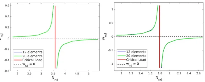
Two types of meshes used within this work are illustrated in Figure 5. The first one has 12 elements (3 elements per side), Figure 5a and the second has 20 elements (5 elements per side), Figure 5b.
Figure 5: Boundary Element Mesh
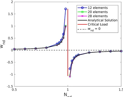
6.1 Isotropic simply supported multicompressed plate
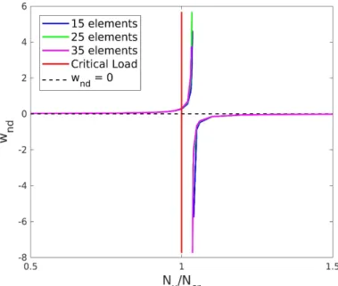
The first problem analyzed was a simply supported square plate of side a = 1m and thickness h = 0.01m. The material properties are E = 200GPa and ν = 0.3. In order to verify the precision of the solution, the displacement of the plate’s center point has been compared with the analytical solution given by Timoshenko and Woinowsky-Krieger (1959). Applying
N
y
N
cr andN
x
0.9
N
cr, the displacement using a 20 elements mesh is5
1.1488797 10
w
m, while the analytical isw
1.1295666 10
5 m which represents an error of 1.71%. If a 28 elements mesh is used, the displacement isw
1.1365988 10
5m with an error of 0.62%. It can be seen that a good agreement is obtained with a 20 elements mesh and the error is reduced as the number of elements increase. Figure 6 shows the displacement of the same plate with two meshes and a variableN
x. The asymptoptic behaviour of the plate’s displacement at the critical load can be clearly seen in Figure 6. Near the critical load the proposed solution has a poor performance with only 3 elements per side (12 elements mesh), but is in good agreement with the series solution of Timoshenko and Woinowsky-Krieger (1959) with the 20 elements mesh.6.2 Isotropic multicompressed plate – other boundary conditions
Liew and Wang (1995) used the Rayleigh-Ritz method to analyze the buckling of some multicompressed plates. They presented results for several cases of polygonal plates with constant linear distributed load perpendicular to the plate’s edges (see Figure 7). For the case of square plates, Nx Ny N .
Figure 7: Square plate compressed in x and y direction.
Table 1 presents the load factors obtained with the proposed solution with different boundary conditions. The following material properties are E = 200GPa, and ν = 0.3. The results are compared with the load factors of Liew and Wang (1995). With the 12 elements mesh most cases present a difference lower than 1%. The critical load in the formulation presented is calculated using the displacement. The case with only one edge clamped is the one that presents the most difficult convergence, but refining the mesh the difference decreases. Applying a 20 elements mesh the difference is approximately 2.29% and with a 28 elements mesh the difference is around 1.66%.
Table 1: Comparisons of buckling load factor Boundary
Condition
BEM Solution 12
elements Difference [%]
CCCC 13.088 0.10
CCSS 8.0106 0.2
FFFC 0.6089 3
FFCC 1.4368 0.65
6.3 Geometry influence on the critical buckling load on isotropic plates
A simply supported square plate has been bevelled to assess the influence of the geometry on the critical buckling load. The cases analyzed are illustrated in Figure 8.
To analyze these cases we assume, Ny Nxy 0 and
N
x varying from 50% to 150% of the critical buckling load. The material properties are the same as in the previous examples and a mesh with 3 elements per edge was used herein.The effect of the bevels in the critical buckling load can be seen in Figure 9. As expected, the critical buckling load is increasing with the reduction of the square plate’s area when compared with the analytical solution of a simply supported square plate.
Figure 9: Critical buckling loads of the beveled isotropic plates
The critical load increase for case I is around 3.8%, which is less than the reduction of the area that is of 4.5%. Whilst cases II and III have the same area, both present different critical loads. Case II rises the critical load in approximately 6.4% and case III has an increase of approximately 8%, which is almost the reduced area for both cases, 9%. This difference is probably due to the symmetries present in case III. Case IV, similar to case I, presents an increase of approximately 12.6%, less than the area reduction (13.5%). The increase in the critical buckling load for case V (approximately 17.6%) is close to the area reduction (18%).
Refining the mesh, the critical load presents values of approximately 3.4% for case I (Figure 10) and 8% for case III (Figure 11), with a 7 elements mesh per side for both cases.
Figure 11: Convergence Study Case III
6.4 Compressive in-plane forces combined with shear in-plane forces for isotropic plates
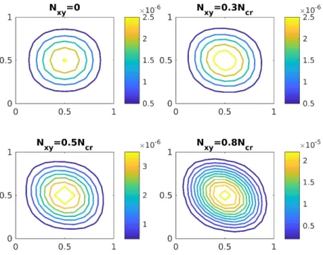
In order to assess the effect of the shear in-plane forces applied together with compressive forces a clamped square plate has been analyzed. In this case Ny Ncr , Nxy Ncr and Nx variable, with Ncr representing the critical buckling load of the bicompressed case. The plate’s dimension are a = b = 1 m, h = 0.01m and the material properties are E = 200GPa and
0.3
.Figure 12 and Figure 13 show the effects of the shear in-plane force on the plate’s displacement field with
0,0.3,0.5,0.8
and a 12 elements mesh. The plate’s deflection is increased with the presence of
N
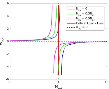
xy and thedisplacement field is distorted (a rotated ellipsis). Figure 14 shows the effect in the critical buckling load. As expected, the critical load is reduced with the increase of Nxy. With 0.3, the reduction was approximately 3%
and with 0.5 the critical load was reduced by approximately 8%.
Figure 13: Displacement fields of a clamped square plate.
Figure 14: Critical buckling load of a clamped square plate with combined compressive and shear in-plane forces.
6.5 Orthotropic plates
Displacement curves for the case where there are in-plane forces and out-plane forces acting on the plate are not available in the literature. Lekhnitskii (1968) developed a series solution for the case of orthotropic plates with a constant distributed out-of-plane force.
A simply supported square orthotropic plate of 1m dimension, thickness, h = 0.01m, material properties
200
l
Lekhnitskii (1968) also developed solutions for the critical buckling load of some unidirectionally and bidirectionally compressed plates. Parameters for the three problems are the following: SSSS unidirectionally compressed and bicompressed. Figure 15 illustrates numerical BEM results for the buckling loads for three problems that have been analytically studied by Lekhnitskii. Using the 12 elements mesh for a square plate with 1m dimension, h = 0.01m,
E
l
20
GPa,E
t
100
GPa,G
lt
38,46
GPa,
lt
0.3
and a perturbation in the form of a concentrated force ofq
1
N.Figure 15: Critical buckling loads for orthotropic plates
6.6 Symmetric laminated plates
Shojaee et al. (2012) applied the FEM to analyze several symmetric laminates compressed in the x direction. The material properties and geometry are: a = b =10m, h = 0.06m, El/Et = 2.45, Glt/Et = 0.48,
lt
0.23
. The buckling load factor is defined as
Nb
2/ (
2D
0,1)
, with D0 ,1 defined as the flexural rigidity along the fiber direction of a plate with a 0° angle ply. Table 2 shows the buckling load factors with a 12 BEM elements mesh for different configurations of ply orientation angles. The BEM proposed solution shows good agreement with FEM results.Table 2: Buckling load factor of laminates
Laminated Method SSSS CCCC Boundary Conditions CSCS SCCS [0°,0°,0°] Shojaee et al. (2012) 2.36 6.71 4.27 3.93
BEM 2.36 6.727 4.27 3.93
[15°,-15°,15°]
Shojaee et al.
(2012) 2.43 6.57 4.41 3.96
BEM 2.426 6.57 4.399 3.94
[30°,-30°,30°]
Shojaee et al.
(2012) 2.59 6.29 4.79 4.00
BEM 2.577 6.258 4.742 3.98
[45°,-45°,45°]
Shojaee et al.
(2012) 2.66 6.10 4.78 4.01
BEM 2.646 6.10 4.828 3.989
[90°,0°,90°] Shojaee et al. (2012) 2.36 6.70 4.36 3.93
6.7 Influence of the angle ply on the critical load of an orthotropic plate
Figure 16 illustrates the critical load of a simply supported square plate with 1x1m, h = 0.01m, El = 200GPa, Et = 100GPa, Glt = 20GPa, νlt = 0.25 for different angle plies. The greatest increase in the critical load has been found for a 45° angle ply in the present example, around 35% increase. We see that the fibers' angle ply has an important effect on the critical load. This effect is highlighted in Figure 17, which illustrates the displacement behavior of the plate with a 0° ply-orientation angle compared to the plates with 30° and 60° ply-orientation angles. The here developed fundamental solution can be used as a tool for optimizing the stability project of laminated polygonal plates.
Figure 16: Critical buckling load of a simply supported square plate with different angle plies.
6.8 Geometry influence on the critical buckling load of orthotropic plates
The same geometries of the isotropic case were studied for an orthotropic plate. The properties for this case are
E
l
200
. GPa,E
t
20
GPa,G
lt
7.69
GPa
lt
0.3
. Figure 18 illustrates the plate’s displacement. The same effect of the isotropic case is observed in the orthotropic case. However, the increase in the critical buckling load for the orthotropic plate are greater than for the isotropic case. The orthotropic critical buckling loads have been increased approximately by 5%, 15%, 16%, 20%, and 31% for each case respectively with 3 elements per edge. This difference is probably due to the differences between the elastic modulus along the fiber and the elastic modulus transversal to the fiber. Refining the mesh, case I tends to decrease the critical load by approximately 3.5% (Figure 19) whilst case III decrease to approximately 15% (Figure 20).Figure 18: Critical buckling load for beveled orthotropic plates
Figure 20: Case III convergence
7 Conclusions
We have developed new fundamental solutions using the Radon transform to solve the buckling problem for isotropic and anisotropic plates under the combined action of in-plane compressive forces/shear forces and out-of-plane loads. Several numerical examples were shown for isotropic, orthotropic, symmetric laminated and monoclinic materials with different boundary conditions and geometries. The results obtained were compared with available analytical solutions and numerical results in the literature. The present formulation can be used without domain integrals for the case of concentrated loads. As long as 0, this BEM solution can be used with the
Appendix A – D Expressions.
2
1 ,
2 3 2 2 2 3 3
, , , , , , 2
1
2 2 1 1
8
1 2 (1 ) (2 3 ) 3
8
y y y ì
x
x y x x y y x y x y x y y x xi
D n r n
N
n r n n n r r r n n r r n n n
D
r n r n
(A1)
2 22 , , , , ,
2 2 3 2 2 2
, , , ,
2 2 2
, , , ,
2
, 1
2 2 1 1
8
1 1 3 2 3
8
1 2 2 1 1
8 1
2 2 1 1
8
y x x y y y x y y xi
x y x x y x y y x y xi
x y x y x y x y yi
y y y ì
D r n r r n n r r n n
r r n n n r r n n n n
r n r r n n r n n
n r n
r n r n
(A2)
2 2 2 2 3 2
3 , , , ,
2 2 2 3 2 2 2
, , , , ,
2 2 2 3 2 2 2
, , , , ,
(1 )
3 2 1 2 3 1 2
8
2 3 3
2 3 3
x y y x y y x y x y ì
y x x x y y x y x y y xi
x y x x y x y x x y y yi
D n n r r r n n n n r
r r n n n r r r n n n n r r n n n r r r n n n n
r n (A3)
2 4 ,2 3 2 2 2 3 3
, , , , , , 2
1 2 2 1 1
8 1
2 (1 ) (2 3 ) 3
8
y y y xi
x
x y x x y y x y x y x y y x ì
D n r n n
N n r n n n r r r n n r r n n
D r n
r n (A4)
2 2 2 2 3 2
5 , , , ,
2 2 2 3 2 2 2
, , , , ,
2 2 2 3 2 2 2
, , , , ,
(1 )
2 3 2 1 2 3 1 2
8
12 4 2 3
12 4 2 3
x y y x y y x y x y ì
y x x y x y x y x y y xi
x y x y x x y x x y y yi
D n n r r r n n n n r
r r n n n r r r n n n n
r r n n n r r r n n n n
References
Albuquerque, E. L., Sollero, P., Venturini, W. S., Aliabadi, M. H. (2006). Boundary element analysis of anisotropic Kirchhoff plates. International Journal of Solids and Structures. 43:4029-4046.
Altiero, N. J., Sikarskie, D. L. (1978). A boundary integral method applied to plates of arbitrary plan form. Comp. & Struct. 9:163-168.
Baiz, P. M., Aliabadi, M. H. (2007). Buckling analysis of shear deformable shallows shells by the boundary element method. Engineering Analysis with Boundary Elements. 31:361-372.
Bézine, G. P. (1978). Boundary integral formulation for plate flexure with arbitrary boundary conditions. Mech. Res. Comm. 5:197-206.
Christensen, R. M. (1979). Mechanics of Composite Materials. Dover Publications, Inc.
Dirgantara, T., Aliabadi, M. H. (1999). A new boundary element formulation for shear deformable shells analysis. International Journal for Numerical Methods in Engineering. 45:1257-1275.
Dirgantara, T., Aliabadi, M. H. (2006). A boundary element formulation for geometrically nonlinear analysis of shear deformable shells. Computer Methods in Applied Mechanics and Engineering. 195:4635-4654.
Ferreira, A. J. M., Castro, L. M. Roque, C. M. C., Reddy, J. N., Bertoluzza, S. (2011). Buckling Analysis of laminated plates by wavelets. Computers and Structures. 89:626-630.
Helgason, S. (1980). The Radon Transform. Birkhäuser.
Herakovich, C. T. (1998). Mechanics of Fibrous Composites. John Wiley & Sons, Inc.
Jahanshahi, A., Dundurs, J. (1964). Concentrated forces on compressed plates and related problems for moving loads. Journal of Applied Mechanics. 31:83-87.
Katsikadelis, J. T., Babouskos, N. G. (2009). Nonlinear Flutter Instability of Thin Damped Plates. Journal of Mechanics Materials and Structures. 4 (7-8):1395-1414.
Kutt, H. R. (1975a). Quadrature Formulae for Finite Part Integrals. The National Research Institute for Mathematical Sciences. Report WISK 178.
Kutt, H. R. (1975b). On the Numerical Evaluation of Finite Part Integrals Involving an Algebraic Singularity. The National Research Institute for Mathematical Sciences. Report WISK 179.
Lekhnitskii, S. G. (1968). Anisotropic Plates. Gordon Breach Science Publishers.
Liew, K. M., Wang, C. M. (1995). Elastic buckling of regular polygonal plates. Thin-Walled Structures. 21:163-173. Ludwig, D. (1966). The Radon transform on Euclidian space*. Communications on Pure and Applied Mathematics. 19:49-81.
Manolis, G. D., Rangelov, T. V., Shaw, R. P. (2003). The non-homogeneous biharmonic plate equation: Fundamental solutions. International Journal of Solids and Structures. 40:5753-5767.
Monteiro Jr., J., Daros, C. H. (2017). Buckling Analysis of Thin Kirchhoff Plates Unidirectionally Compressed via the Boundary Element Method. In: Proceedings of International Symposium on Solids Mechanics – MecSol, 6., Joinville – Brazil: ABCM.
Paiva, J. B., Venturini, W. S. (1992). Alternative Technique for the Solution of Plate Bending Problems Using the Boundary Element Method. Advances in Engineering Software. 14:265-271.
Rangelov, T. V., Manolis, G. D., Dineva, P. S. (2005). Elastodynamic Fundamental Solutions for Certain Families of 2d Inhonogeneous Anisotropic Doamians: Basic Derivations. European Journal of Mechanics A/Solids. 24:820-836. Shi, G (1990). Flexural vibration and buckling analysis of orthotropic plates by the boundary element method. International Journal of Solids Structures. 26:1351-1370.
Shi, G., Bézine, G. P. (1990). Buckling analysis of orthotropic plates by boundary element method. Mechanics Research Communications. 17:1-8.
Shojaee, S., Valizadeh, N., Izadpanah, E., Bui, T., Vu, T. V. (2012). Free vibration and buckling analysis of laminated composite plates using NURBS-based isogeometric finit element method. Composite Strucutres. 94:1677-1693. Stern, M. A. (1979). A general boundary integral formulation for the numerical solution of plate bending problems. Int. J. Solids Struct. 15:769-782.
Syngellakis, S., Elzein, A. (1994). Plate Buckling Loads by The Boundary Element Method. International Journal for Numerical Methods in Engineering. 37:1763-1778.


![Table 1: Comparisons of buckling load factor Boundary Condition BEM Solution elements 12 Difference [%] CCCC 13.088 0.10 CCSS 8.0106 0.2 FFFC 0.6089 3 FFCC 1.4368 0.65](https://thumb-eu.123doks.com/thumbv2/123dok_br/16310743.718340/13.892.207.676.777.1138/table-comparisons-buckling-boundary-condition-solution-elements-difference.webp)