Abstract
This work reviews the developments of Boundary Element Method formulations to solve several types of plate bending problems, including non-linear bending. The formulation is developed and solved using the standard BEM procedure, and different integration approaches were discussed and tested. Object oriented implementa-tion issues are commented. Results were obtained for linear and non-linear elastic bending as well as buckling of selected cases of thick plates, including cases of step variation in thickness under large displacements regime.
Keywords
Boundary element method, thick plate, nonlinear plate bending, plate buckling, object oriented programming.
Revisiting Some Developments of Boundary
Elements for Thick Plates in Brazil
1
1 INTRODUCTION
Traced back to early 1980’s, the development of general boundary element approaches for thick
plate bending analysis took almost fifteen years to be fully established. This was partly due to the numerical and mathematical difficulties that have been preventing a more general use of the boundary element method (BEM) to complex problems like dynamical and non-linear problems, but also intrinsically related to the complex nature of plate/shell equations, arguably some of the most challenging among the usual structural theories. The first work on the application of the BEM to moderately thick plates was published in 1982 (van der Weeën, 1982). In spite of several other published works on the matter during the last decades, there are still few works dealing with non-linear bending (Vilmann, 1990) (Xiao-Yan et al., 1990)(Marczak, 2004)(Supriyono, 2006), contact problems, anisotropic material, and variable thickness problems (di Pisa, 2005), to name a few
1Much of the work presented here was developed or started its development during the 1990s during the
collabo-ration of the author with Prof. Clóvis S. de Barcellos, and has been under continuous improvement since then. The present review not only summarizes an important research branch of boundary element methods, but also recognizes the pioneering vision of Prof. Barcellos in encouraging a whole generation of then young researchers to pursuit challenging problems, and solve them under well posed formulations.
Rogério José Marczak
Mechanical Engineering Dept. - UFRGS Rua Sarmento Leite 425, Porto Alegre, Brazil – 90050-170
http://dx.doi.org/10.1590/1679-78251441
Latin A m erican Journal of Solids and Structures 12 (2015) 948-979 shear deformable plate research topics solved by the BEM. Characteristics of the BEM in plate bending analysis like the absence of locking and the high accuracy moments and shear forces are among the advantages that justify further works on the subject.
This work collects the relevant boundary element equations for linear and non-linear bending as well as buckling analysis of moderately thick plates. The plate models account for the shear influ-ence by using the Mindlin and the Reissner first order plate theories. A unified integral formulation for the plate models is extended to the differential operators found in von Kármán equations in order to consider geometrically non-linear effects. The integral formulation for membrane-bending coupling is also developed, leading to an integral equation system that describes large displacement bending problems. The linearization of these equations leads to an eigenproblem which can be used for the linear elastic stability analysis. Yet another special case of these equations leads to a linear system corresponding to the boundary value problem of static bending of plates. The direct bound-ary element method was used to obtain an approximate solution of the integral equation system. The proposed formulation was tested using constant, linear and quadratic elements for non-linear benchmark cases, and up to quartic elements for linear tests.
Most of the present work started back in 1990 in a research group at Federal University of San-ta CaSan-tarina, Brazil. At t—e time, improvements on van der Wëeen’s work (1992) on Reissner’s plate were done and extended to linear bendin– of Mindlin’s plate model (de Barcellos & Monken e Sil-va1, 1989)(de Barcellos & Westphal Jr., 1992) (Westphal Jr. & de Barcellos, 1990), buckling (Marczak, 1995b, 1995c), higher order elements (Marczak, 1995a). Later non-linear bending was also explored at Federal University of Rio Grande do Sul ((Marczak, 1996) (Marczak & Creus, 2002). Meanw—ile, plastic bendin– of Reissner’s plate were solved at Federal University of Rio de Janeiro (Karam & Telles, 1988), while other groups kept developing the method for thin plates (Costa Jr. & Brebbia, 1985) (Chaves et al., 1999)
The integral formulation presented herein is condensed to account for a general boundary inte-gral equation framework of elastic analysis of moderately thick plates. The numerical examples presents novel figures for a selection of benchmarks, and compare the h convergence rates for boundary elements ranging from constant up to quartic degree with several progenitors of now re-nowned finite elements. Results comparing three singular integration schemes also provide a useful set of reference results to assess other numerical formulations. BEM results for thick plate buckling and non-linear bending of plates with varying thickness seem to be original in the BEM context as well.
2 NAVIER EQUATIONS FOR FOSD PLATE THEORIES
The displacement field usually employed in the first order shear deformation (FOSD) theories, like the Mindlin (1951) plate theory, in conjunction with the 2D elasticity (membrane) equations, is based in the following expansions for the displacements 2:
2Index notation is used throughout this work. Greek indexes range from 1 to 2 while the Latin ones range from 1
Latin A m erican Journal of Solids and Structures 12 (2012) 948-979
1 2 3 3
3 1 2 3 3
,
,
,
,
U
x x x
v
x u
U
x x x
u
(1)Where v and u are the membrane and plate displacements, respectively (i.e.
v
andu
3 are the in plane and out of plane translations, respectively, whileu
are the plate rotations). All variables arereferred to the plates's middle surface. The Reissner's plate model (Reissner, 1944, 1945) also leads to eqs.(1) when the mean value of the displacements is taken across the thickness. Substituting eqs.(1) in the finite deformations strain tensor and neglecting the thickness extensibility, the strain-displacement relations are obtained. When these are used in the generalized Hooke's law and inte-grated through the thickness leads to the constitutive equations of the problem:
3, 3,, , 3, 3, ,
, , , 2 3,
1
2
2
1
2
2
1
1
,
2
u u
N
C
v
v
u u
C
v
M
D
u
u
u
Q
D
u
u
(2)where
C
Eh
/ (1
2)
,D
Eh
3/12(1
2)
, 2 2 212
/
h
andh
is the plate thickness, while
2is the shear correction factor used to weight the values of the transverse shear stress
3. The equilibrium equations are obtained from the Principle of Virtual Work and written in terms of re-sultant stress:
,
3, , , 3
,
0
0
0
N
f
N u
Q
q
M
Q
m
(3)where
N
are the in-plane (membrane) forces,Q
are the shear forces andM
are the bendingmoments. The symbols
f
andq
3 stand for the in-plane and transverse loadings, respectively, whilem
are the distributed moments. The boundary conditions associated to eqs.(3) are of three types, namely, in-plane (l
), out of plane (t
3) and binaries (t
), given by:3 3,
3 3,
at
, or
at
at
, or
at
,
at
, or
at
,
u t
u
t
u t
l
N n
l
N n
t
N u n
Q n
t
N u n
Q n
t
M n
t
M n
Latin A m erican Journal of Solids and Structures 12 (2015) 948-979
where
u is the portion of the boundary where the Dirichlet boundary conditions are imposed, whereas
t is the portion where the Neumann boundary conditions are specified, and n is the out-ward vector normal to the boundary. Aiming an unified numerical implementation for both plate models the expression for the moments is rewritten with an additional term (Westphal Jr. et al., 1998):, , , 3
1
2
.
2
1
fM
D
u
u
m q
(5)where 2
/ (1
)
f
m
for the Reissner's plate model andm
f
0
for the Mindlin's model. It is convenient to distinguish the linear and the non-linear parts:l n
l n
N
N
N
Q
Q
Q
(6)so that
, , ,
3, 3, 3, 3,
2 3, 3,
1
2
2
1
1
2
1
1
2
,
l n l nN
C
v
v
v
N
C
u u
u u
Q
D
u
u
Q
N
u
(7)The Navier equations are found by substituting the above equations for N , M , and Q in eqs.(3), and transferring all the non-linear terms to the loading terms, leading to the following general form:
m
m m
f f f
q
L
0
u
0
L
u
q
(8)Where m
L
is the differential operator of the linear membrane equilibrium problem, fL
is the line-ar bending operator, mu
{
v v
1 2}
T are the in-plane displacements and fu
{
u u u
1 2 3}
T are the plate displacements. The membrane-bending coupling is implicit in the corresponding pseudo-loadings mˆ
q
and fˆ
q
, because mq
n needs the derivatives of the transverse displacement in itsevalua-tion, and f
q
n uses the membrane stresses (see definitions for the non-linear parts):(
)
( )
( )
(
)
( )
( )
m m m l m n
Q
f f f l f n
ij Q j i i
q
F
q Q
q Q
q
F
q Q
q Q
Latin A m erican Journal of Solids and Structures 12 (2012) 948-979
The complete expressions of the terms used in Eqs.(8) and (9) are given by:
2 2
2
1 1 2
2 2
2
1 2 2
2 2
2 2
2
1 1 2 1
2 2
2 2
2
1 2 2 2
2 2 2
1 2
1
(
)
2
1
(
)
2
m Q f Qx
x x
C
x x
x
x
x x
x
D
x x
x
x
x
x
L
L
1 21
0
(
)
0 1
1
0
(
)
0 1
0
0 1
m Q f f Q f
m
x
m
x
F
F
1 1 2 2 1 23, 3, , 3, 3, ,
3, 3, , 3, 3, ,
( )
(
)
(
)
1
1
( )
2
(
)
(
)
1
T m l m nQ
f
f
u u
u u
Q
C
u u
u u
q
q
1 2 3
3, ,
( )
1
( )
0
0
(
)
2
T f l
T f n
Q
q
q
q
Q
D
N u
q
Latin A m erican Journal of Solids and Structures 12 (2015) 948-979
where
1
/ 1
and
2/ (
x x
)
. Equations (8) describe an in-plane elastic prob-lem coupled to a moderately thick plate elastic bending probprob-lem due to the consideration of large displacement terms.3 NUMERICAL IMPLEMENTATION
By means of the weighted residual method, the following Somigliana identities are obtained for eqs.(8), using the steps detailed in Marczak (1998, 2004):
,
( ) ( )
( , ) ( )
( , ) ( )
( , )
( )
( , )
( )
( ) ,
m m m
q q
m
Q
m n m
Q
C
p v p
T
q p v q d
U
q p l q d
V
Q p f Q d
U
Q p N
Q d
v
p
(10) and 3, 3,( )
( )
( , )
( )
( , ) ( )
( , )
( )
( , )
( )
( )
( ) ,
f f f
ij j ij j q ij j q
f
ij j Q
f f
i Q i
C
p u p
T q p u q d
U q p t q d
V Q p q Q d
U
Q p N
Q u
Q d
v p
(11)for the membrane and the bending problem, respectively. The non-integral terms m
v
and fv
iwere included to account for concentrated loads inside the domain (Kamiya & Sawaki, 1985). The symbols p and q denote source (collocation) and field points, respectively (lower case indicates boundary points and upper case indicates domain points). The corresponding displacement ( m
ij
U
and f ij
U
) and traction ( m ijT
and f ijT
) fundamental solutions can be found elsewhere (de Barcellos & Westphal Jr., 1992)(Westphal et al., 2001). Eqs.(10) and (11) can be particularized for internal points by making mC
and fC
ij
ij. They require the evaluation of the deriva-tives of the transverse displacement which are present in the nonlinear membrane forces of the last integrals of both. These terms are partially resposible for the membrane-bending coupling. In that non-linear form, eqs.(10-11) were first derived by the author (Marczak, 1998), while its linear form unifying both the Mindlin and the Reissner plate models were first published earlier (de Barcellos & Westphal Jr., 1992). This form uses a factor that specifies which thick plate model is being used, and has been adopted by many researches since then.Latin A m erican Journal of Solids and Structures 12 (2012) 948-979
The use of the derivative boundary integral equations associated to eqs.(10-11) is far more accu-rate than to assume an a priori interpolatory form for the displacements derivatives. Hence a more rigorous solution can be obtained by differentiation of these integral equations with respect to the coordinates
x P
( )
. The procedure leads to six additional integral equations forv
, andu
3,.Assuming that the derivatives fields are required only at internal points, the differentiation of the boundary integrals in eqs.(10-11) under the integration sign is straightforward as their kernels be-come all regular. However, the differentiation of the domain integrals must be treated by means of the Leibnitz formula (Bui, 1978). The formal derivation of such derivative integral equations pro-duce the so called convective terms which must be added to the final expressions for
v
,( )
P
and3,
( )
u
P
, resulting:, , , , , ,
( )
( , ) ( )
( , ) ( )
( , )
( )
( , )
( )
( )
( )
m m q qm m n
Q Q
m N m
v
P
T
q P v q d
U
q P l q d
V
Q P f Q d
U
Q P N
Q d
c
P
v
P
(12)3, 3 , 3 ,
3 , 33, 3,
3, 3,
( )
( , ) ( )
( , ) ( )
( , ) ( )
( , )
( )
( )
( )
( )
( )
f f
i i q i i q
f
i i Q Q
N f
u
P
T
q P u q d
U
q P t q d
V
Q P q Q d
U
Q P N
Q u
Q d
c
P u
P
v
P
(13)where a negative sign was added to all the integrals as the derivatives are taken with respect to
( )
x P
and (Marczak, 2004)
2
1
( )
3 4
8 (1
)
1
1 2
( ) ,
4
( )
( )
(1
)
m N n f Nc
P
G
N
P
c
P
N
P
D
(14)are the aforementioned convective terms. Eqs. (12-13) are truly hypersingular derivative integral equations and, as such, one can expect the same convergence properties of any equilibrium equa-tions written in its strong form.
Latin A m erican Journal of Solids and Structures 12 (2015) 948-979
• Membrane (2D elasticity) problem:
m m
m m
m mH u
G t
B
f
(14)• Bending problem:
3
f f
f f
f
fH u
G t
Bu
f
(15)• In-plane displacements derivatives:
m m
u
H u
G t
B
f
(16)• Transverse displacement derivatives:
3 3 3 3
3 3
.
f f
u
H u
G t
Bu
f
(17)where
1 2
, ,
T
v
v
u
and
1 2
3 3, 3,
T
u
u
u
.3.1 Non-linear Bending
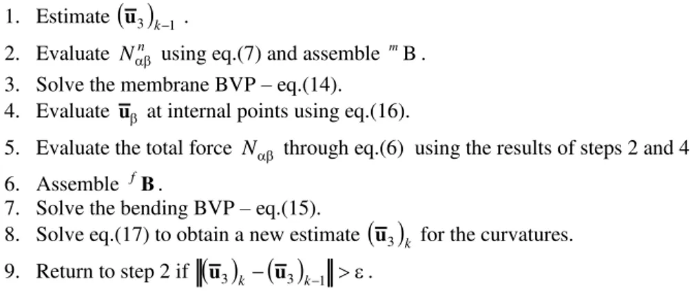
All types of B matrices refer to the membrane-bending coupling, given by the last integral in eqs.(10-13). Equations (14-17) must be solved by an iterative procedure. Figure 1 exemplifies a ge-neric k-th iteration. The convergence was verified against the norm of the curvature error, i.e.
3, 3, 1k k
u u
, since it showed to be dominant in numerical experiments.
The steps 4 and 8 in Fig.1 assume the application of eqs.(16) e (17). Nevertheless, they are very difficult to extend to other applications. For instance, the inclusion of material non-linearities or thermal effects would imply in new integral terms and possibly new convective terms, resulting in a very cumbersome, application specific numerical implementation.
Anticipating the use of discontinuous domain cells - whose physical nodes never rest on the boundary - eqs.(16-17) will be quasi-singular at most, and a finite difference scheme can be used instead of the true derivatives of the displacements. Finally, it is worth to mention that a full up-date of the displacement derivatives enables convergence only for mild nonlinearities, so that a re-laxation factor must be employed at the end of each iteration to stabilize the process:
,
,
,1
1
1i i i
k k k
u
u
u
Latin A m erican Journal of Solids and Structures 12 (2012) 948-979 1. Estimate
u3 k1 .2. Evaluate Nn using eq.(7) and assemble Bm . 3. Solve the membrane BVP – eq.(14).
4. Evaluate u at internal points using eq.(16).
5. Evaluate the total force N through eq.(6) using the results of steps 2 and 4.
6. Assemble fB.
7. Solve the bending BVP – eq.(15).
8. Solve eq.(17) to obtain a new estimate
u3 k for the curvatures.9. Return to step 2 if
u3 k u3 k1 .Figure 1: General algorithm to solve non-linear problems described by eqs. (14-17).
The resulting systems of equations for each class of problem (membrane, bending and displacement derivatives) are summarized below.
3.2 Linear Bending
The equations here are obviously decoupled, and eq.(15) becomes:
.
f f
f f
fH u
G t
f
Collecting plate displacements and tractions in a vector x results: f f
fA x
f
3.3 Linearized Stability
In this case, although there is a coupling between the bending and the plane problems, the latter is parameterized by an in-plane load factor
N
N
, so that the only remaining unknown of the membrane problem is . Therefore the system of equations for buckling problems are derived as particularization of the equations for non-linear bending. Since there is no other loadings, eqs.(15) and (17) are rewritten and regrouped as3
3 3
3
f f f
f
A x
B u
u
A x
B u
When combined, the above equations result the eigenproblem:
3 1 3
3 3
1
f f
A A
B
B u
u
Latin A m erican Journal of Solids and Structures 12 (2015) 948-979
buckling load. Of note is the fact that in BEM, stability problems does not result in a generalized eigenproblem like in FEM, but a classical one encompassing one single matrix. The corresponding displacements for internal points are obtained through the bending Somigliana identity particular-ized for null transverse loading.
3.4 Numerical Integration
Concerning numerical integration of the singular and quasi-singular kernels found in the present formulation, during the early stages of this work in the 1990s, most of the results obtained by the present formulation used to rely on the integration of singular kernels by rigid body movement (RBM) imposition or Kutt's quadrature (Kutt, 1975), while weakly singular kernels were integrated with Telles' cubic transformation (Telles, 1987). Even considering the limitations of both, the re-sults were very good. However, the RBM method always depend on the quality of the integration over the adjunct part of the boundary (although it always guarantees the fulfillment of equilibrium) while Kutt's quadrature is very difficult to be used with curved elements. During early 2000, the authors greatly improved the quality and the extentensibility of the formulation by deriving the asymptotic expansions of the relevant kernels for 2D elasticity and thick plates and implemented the direct method (Guiggiani et al. 1992) (Guiggiani, 1998) to evaluate all strongly singular inte-grals. The efficiency of this approach in regularizing the singular integrals is demonstrated in Marczak & Creus (2002).
4 IMPLEMENTATION ISSUES
The continued development of BEM codes has naturally lead to a demand for extensibility and reusability of the codes (or part of them) without demanding the costs associated to the develop-ment of new software or due to unwanted changes in source codes successfully tested and used. The present work was developed under an object-oriented architecture used as a general numerical framework for the development of computer programs based on boundary integral equation meth-ods. A number of classes were developed to automatize ordinary tasks like collocation procedures, numerical integration, degrees of freedom mapping, among several others. The framework is also capable of handling an arbitrary number of subregions. The design was able to successfully unlink the so-called domain classes (those containing elements, nodes, loads, etc.) from the analysis classes (linear, non-linear, static, transient etc.).
meth-Latin A m erican Journal of Solids and Structures 12 (2012) 948-979
od, including non-linear applications. The underlying idea in its design is that different applications share a common mathematical and numerical structure, and more importantly, storage (model) classes do not perform any solution step. The library provides a complete set of auxiliary and model classes, as well as a basic set of analysis classes. To create an application, the analyst assembles the code by collecting the objects necessary to perform the solution. The programming work is limited to implement the new analysis classes deriving them from any of the existing ones, in case they are not provided. In the presently proposed OO architecture, a tentative organization was advised for the analysis classes (and their descendents) in such a way that the most important analysis tasks are logically grouped regarding the differential equation point of view. In this way, the analyst is able to assemble a code according to the problem to be solved: linear or nonlinear, static or dynam-ic, type of resulting system of equations, solution strategy and so forth. A brief description of some important auxiliary, model and analysis classes used to generate the results of the present work is given below.
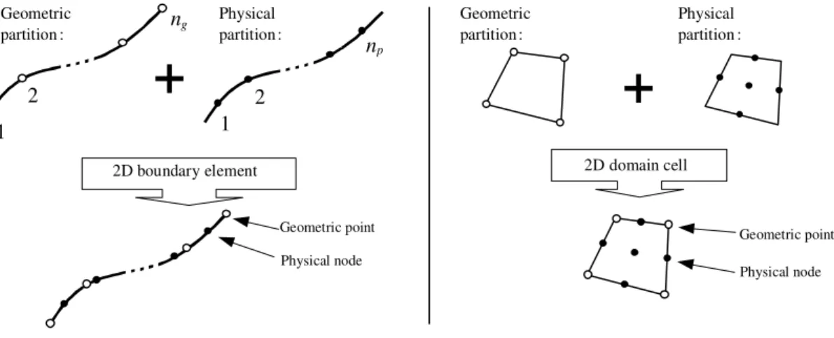
Class mcGeometricPartition: The construction of any domain partition (boundary elements or do-main cells) is based in a composition of geometric and physical partitions (see fig.2). The mcGeometricPartition class implements the topology of the partition. It is composed basically by a list of points and the associated shape functions. This approach enables the implementation of less conventional geometric mappings, like cubic splines and Bézier curves. Methods for evaluation of Jacobians, dimension of the normalized space, mapping to or from the normalized space, etc. are provided. From this superclass other classes used to define lines, areas and volumes descend. For example, mc1DGeometricPartition and mc2DGeometricPartition are used to define lines and areas, respectively.
Class mcPhysicalPartition: Similar to mcGeometricPartition, but in this case the object has the connectivity composed by a list of physical nodes. Examples of its descendents are the mc1DPhysicalPartition and mc2DPhysicalPartition classes, used to implement physical interpola-tions on lines and areas respectively.
Other classes like mcDOF and mcDOFSet encapsulate data for a single degree of freedom and for a list of mcDOF objects. The user can assemble a particular set of variables according to the problem to be solved. For use with the BEM, this class generally encapsulates properties for primal and dual variables, and their derivatives as well.
Latin A m erican Journal of Solids and Structures 12 (2015) 948-979
• Matrix Tensor(char* id, mcCoord& q, Vector& n): Evaluates a fundamental tensor (T,U , etc.) using the current load point.
• Matrix Limit(int ns, char* id, Vector& N, Vector& T, Matrix& Shape, Matrix& dShape): Eval-uates the asymptotic expansions of a tensor to be used in singular integrations.
• Matrix Jump(Vector& ang, char* id): Evaluates the free terms of a tensor. The most common case are the geometric factors. Other types of jump terms can be considered as well.
• mcArray getSingType(char* id): Returns an array of codes corresponding to the type and severi-ty of the singulariseveri-ty of each component of a tensor.
1 2
g
n
Geometric partition :
+
1 2
p
n
Physical partition :
Geometric point
Physical node
+
Geometric partition :
Physical partition :
2D domain cell
Geometric point
Physical node
2D boundary element
Figure 2: Illustration of the composition of two-dimensional domain partitions using geometric and physical partitions.
The analysis of the problem itself is performed by a set of five superclasses aggregated by the ana-lyst, depending on the type of the problem and solution desired. Many of the ideas adopted here were adapted from a previous work on finite elements (McKeena, 1997). This approach is quite flexible as it enables the user to group each of these five major classes according to the specific needs of an application. If necessary, one can implement a new class by deriving it from any of the superclasses and limiting the coding task to those analysis steps not provided by the library.
Latin A m erican Journal of Solids and Structures 12 (2012) 948-979
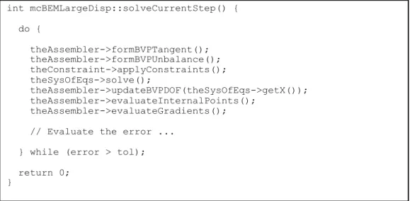
• int solveCurrentStep():Controls the assembly of left and right hand sides of the system of equa-tions for the current time and load steps. In the BEM subclasses, this is generally related to the solution of the associated boundary value problem (BVP). Figure 3 shows a typical implementation of the solveCurrentStep member for linear problems. Its counterpart for nonlinear cases is illustrat-ed in fig.4.
• int postProcessCurrentStep():Performs the post-processing of the current step. For example, in BEM applications the evaluation of the remaining variables at internal points is carried out using this method.
int mcBEMLinear::solveCurrentStep() {
theAssembler->formBVPTangent(); theAssembler->formBVPUnbalance(); theConstraint->applyConstraints(); theSysOfEqs->solve();
theAssembler->updateBVPDOF(theSysOfEqs->getX());
return 0;
}
Figure 3: Code fragment of the solveCurrentStep member for linear applications.
int mcBEMLargeDisp::solveCurrentStep() {
do {
theAssembler->formBVPTangent(); theAssembler->formBVPUnbalance(); theConstraint->applyConstraints(); theSysOfEqs->solve();
theAssembler->updateBVPDOF(theSysOfEqs->getX()); theAssembler->evaluateInternalPoints();
theAssembler->evaluateGradients();
// Evaluate the error ...
} while (error > tol);
return 0; }
Figure 4: Code fragment of the solveCurrentStep member for non-linear applications.
Latin A m erican Journal of Solids and Structures 12 (2015) 948-979
Similar classes can be easily implemented for finite elements. In the current framework, all BEM applications are based on the solution of the boundary value problem and possibly a corresponding domain value problem. It is assumed that even in nonlinear problems, the nonlinear contributions can be included in the right hand side of the system of equations. As a consequence, the relevant methods are those responsible for the assembly of the final solution system of equations. Some of the relevant methods currently implemented are described below.
• int formBVPTangent():Responsible for the assembly of the left hand side of the BVP system of equations. In the BEM, this is generally accomplished by imposing the boundary conditions and grouping the contributions of the matrices H and G during the collocation process. It is worth to note that, unlike most FEM formulations, part of the right hand side is evaluated during this phase.
• int formBVPUnbalance():Here the assembly of the right hand side of the system is finished by adding the domain contributions, such as domain loadings and nonlinear terms. This method is not used in pure boundary value problems.
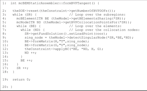
As an example, the basic code of the method formBVPTangent is listed in figs.5. It is worth to point out that, besides their simplicity, these members remain the same for linear and nonlinear applications, provided the nonlinear terms are handled by a member formBVPUnbalance.
Figure 5: Code fragment of the formBVPTangent member for linear static applications.
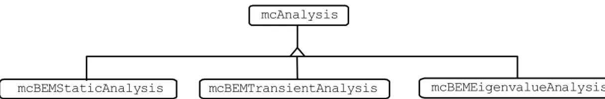
Class mcAnalysis: This is the analysis superclass of the present OO design. A mcAnalysis object is actually an aggregation of the analysis objects described above. In spite of the fact that it does not perform any explicit calculation, the mcAnalysis class defines which type of problem will be solved
1: int mcBEMStaticAssembler::formBVPTangent() {
2: theSOE->reset(theConstraint->getNumberOfBVPDOFs()); 3: while (SR) { // Loop over the subregions: 4: mcBElementITR BE (theModel->getBElementsSharing(*SR)); 5: mcNodeITR ND (theModel->getBVPCollocationPointsFor(*SR)); 6: while (BE) { // Loop over the elements:
7: while (ND) { // Loop over the collocation nodes: 8: SR->getFundSolution().setLoadPoint(coor);
9: sing_node = theModel->detectSingularNode(*SR,*BE,*ND); 10: BE->formMatrix(H,"T",sing_node);
11: BE->formMatrix(G,"U",sing_node);
12: theConstraint->applyBC(*BE, *ND, H, G); 13: ND ++;
14: } 15: BE ++; 16: }
17: SR ++; 18: }
19: return 0;
Latin A m erican Journal of Solids and Structures 12 (2012) 948-979
and how. It is also responsible for checking the validity of the objects in the aggregation so that it makes sense. A single virtual method called analyze() triggers the analysis execution. The computa-tional model is constantly checked to verify if another analysis is necessary. Figure 6 shows some examples of analysis subclasses derived in the present work.
mcAnalysis
mcBEMStaticAnalysis mcBEMTransientAnalysis mcBEMEigenvalueAnalysis
Figure 6: The two major hierarchy levels of the mcAnalysis class.
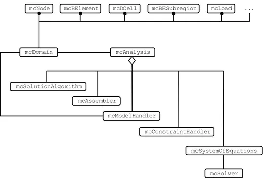
The classes introduced in this work can be used in an stand-alone fashion as tools incorporated to other computer codes. But the advantages of the suggested approach become more evident when all the major classes are connected to generate a given application. Figure 7 depicts a diagram of a complete application, showing the relationship between the major classes. Although other variations are possible, this basic framework has been proving to be sufficiently general for most cases.
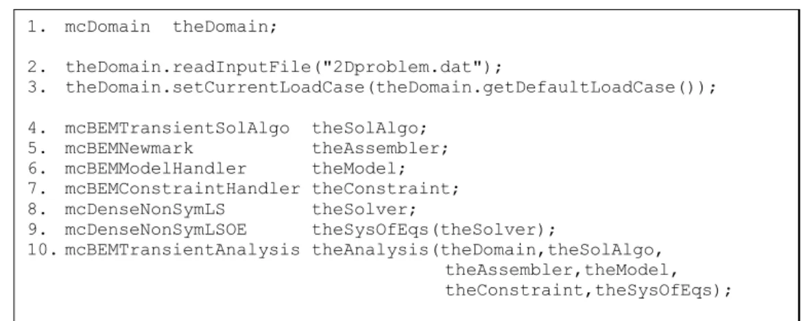
One of the main goals of the OO design proposed in this work is to enable the analyst to write a few programming lines to built a basic BEM code, and yet be able to customize the code for other applications with little additional programming effort. Thus, even more complex analysis would be straightforward reusing the relevant objects. For example, if the analyst were interested in a linear elastic analysis, then the code fragment shown in fig.19 would suffice. Note that the solution of, say, a linear static plate bending or a steady state heat conduction problem would use the same code (the inherent differences are hidden in the subregion objects). But if the interest is to solve the same problem using a dynamic transient analysis, it is necessary to change only lines 4, 5 and 10 in the original code of fig.19 according to fig.20.
Latin A m erican Journal of Solids and Structures 12 (2015) 948-979 mcAnalysis
mcDomain
mcSolutionAlgorithm
mcAssembler
mcModelHandler
mcConstraintHandler
mcSystemOfEquations
mcSolver mcNode mcBElement mcDCell mcBESubregion mcLoad ...
Figure 7: Minimal class diagram of a complete application code.
1. mcDomain theDomain;
2. theDomain.readInputFile("2Dproblem.dat");
3. theDomain.setCurrentLoadCase(theDomain.getDefaultLoadCase());
4. mcBEMLinear theSolAlgo; 5. mcBEMStaticAssembler theAssembler; 6. mcBEMModelHandler theModel; 7. mcBEMConstraintHandler theConstraint; 8. mcDenseNonSymLS theSolver;
9. mcDenseNonSymLSOE theSysOfEqs(theSolver);
10.mcBEMStaticAnalysis theAnalysis(theDomain,theSolAlgo, theAssembler,theModel, theConstraint,theSysOfEqs);
11.theAnalysis.analyse();
Latin A m erican Journal of Solids and Structures 12 (2012) 948-979
1. mcDomain theDomain;
2. theDomain.readInputFile("2Dproblem.dat");
3. theDomain.setCurrentLoadCase(theDomain.getDefaultLoadCase());
4. mcBEMTransientSolAlgo theSolAlgo; 5. mcBEMNewmark theAssembler; 6. mcBEMModelHandler theModel; 7. mcBEMConstraintHandler theConstraint; 8. mcDenseNonSymLS theSolver;
9. mcDenseNonSymLSOE theSysOfEqs(theSolver);
10.mcBEMTransientAnalysis theAnalysis(theDomain,theSolAlgo, theAssembler,theModel, theConstraint,theSysOfEqs);
11.theAnalysis.analyse();
Figure 9: Code for a BEM transient dynamic analysis.
Finally, another interesting feature of the present class library is the ability to integrate any alge-braic type of integrand and handle singular integrals. The former can be accomplished by using fully template-based definitions. This leads to the concept of numerical integration of objects, which would allow a member function of an arbitrary object to be integrated (provided it overloads the basic algebraic operations) as a Riemann sum:
K
i
i i w
d
1 1
1Object( ) Object( ) Result
Latin A m erican Journal of Solids and Structures 12 (2015) 948-979
(”T” for t—e traction fundamental solution T etc.). The member applyBC invoked in line 10 enforc-es the boundary conditions to generate the final system of equations.
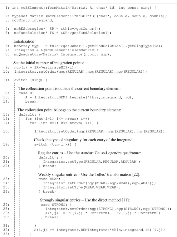
Unfortunately, not all fundamental solution tensors behave with the same degree of singularity for all its components. For instance, in the traction fundamental solution of the Mindlin plate mod-el all the components are either regular or weakly singular except for
T
12 andT
21 which are strongly singular. In such cases, a single call to the NIntegrate member function in order to inte-grate the whole (matrix) kernel at once would not work properly.1: be = BEMModel->getBElements();
2: nd = BEMModel->getBVPCollocationPoints();
3: while (be) { // Loop over the elements:
4: while (nd) { // Loop over the collocation nodes: 5: fundamental_solution = be.current->getFundSol();
6: fundamental_solution.setLoadPoint(nd.coor()); 7: sing_node = BEMModel->detectSingularNode(*be,*nd); 8: be->formMatrix(H,"T",sing_node);
9: be->formMatrix(G,"U",sing_node);
10: theConstraint->applyBC(*be, *nd, H, G); 11: nd ++;
12: } 13: be ++; 14: }
Figure 10: Code excerpt showing the integration and assembly of typical BEM matrices.
Latin A m erican Journal of Solids and Structures 12 (2012) 948-979
1: int mcBElement::formMatrix(Matrix& A, char* id, int const sing) {
2: typedef Matrix (mcBElement::*mcBEInt3)(char*, double, double, double); 3: mcBEInt3 integrand;
4: mcBESubregion* SR = &this->getOwner(); 5: mcFundSolution* FS = &SR->getFundSolution();
Initialization:
6: mcArray typ = this->getOwner().getFundSolution().getSingType(id); 7: integrand = &(mcBElement::elemMatrix);
8: mcQuadrature<Matrix> Integrator(ncoor, nip);
Set the initial number of integration points:
9: ngp(i) = SR->estimateNIP(i);
10: Integrator.setOrder(ngp(REGULAR),ngp(REGULAR),ngp(REGULAR));
11: switch (sing) {
The collocation point is outside the current boundary element:
12: case 0:
13: A = Integrator.BEMIntegrate(*this,integrand, id); 14: break;
The collocation point belongs to the current boundary element:
15: default: {
16: for (int i=1; i<= nrows; i++) 17: for (int k=1; k<= nrows; k++) {
18: Integrator.setOrder(ngp(REGULAR),ngp(REGULAR),ngp(REGULAR));
Check the type of singularity for each entry of the integrand:
19: switch (typ(i,k)) {
Regular entries – Use the standart Gauss-Legendre quadrature:
20: default : {
21: Integrator.setType(REGULAR,REGULAR,REGULAR); 22: } break;
Weakly singular entries – Use the Telles’ transformation [22]:
23: case WEAK: {
24: Integrator.setOrder(ngp(WEAK),ngp(WEAK),ngp(WEAK)); 25: Integrator.setType(WEAK,WEAK,WEAK);
26: } break;
Strongly singular entries – Use the direct method [11]:
27: case STRONG: {
28: Integrator.setOrder(ngp(STRONG),ngp(STRONG),ngp(STRONG)); 29: A(i,j) += F1(i,j) * CorrTerm1 + F2(i,j) * CorrTerm2; 30: } break;
31: }
32: A(i,j) += Integrator.BEMIntegrate(*this,integrand,id)(i,j); 33: }
34: } 35: break; 36: }
Add the Cij terms for the singular elements:
37: if (sing) this->addJumpTerm(A, id, sing, angle);
38: return 0; 39: }
Latin A m erican Journal of Solids and Structures 12 (2015) 948-979
5 RESULTS
The numerical examples presented in this section represent a selection of benchmarks typically used to show the quality of the results in several plate formulations. Results are presented for three groups of problems: linear bending, buckling, and non-linear bending. They not only allow a verifi-cation of the accuracy of the BEM scheme described in section 3, but also compare the h conver-gence rates for boundary elements ranging from constant up to quartic degree with several progeni-tors of now renowned finite elements. To t—e aut—ors’ knowled–e, t—is —as never been publis—ed for plate problems in the open literature. Another important class of results shown herein compares all three singular integration schemes developed, and they provide a useful set of reference results for comparison with other numerical formulations, therefore extensive use of tabular results was also made. BEM results for thick plate buckling is another kind of result seldom presented in the litera-ture. The results for non-linear bending of plates with varying thickness seem to be original in the BEM context as well.
Unless specified otherwise, the results presented herein employ the Mindlin's model with the following non-dimensional data: Young modulus
E
3.0 10 ,
6 Poisson coefficient
0.30
, shear correction factor 2 2/12
, lateral loading (when applicable)
q
3
1000
, lateral dimension of square plates or radius of circular platesa
1.0
. It is well known that the FOSD plate theories enable the imposition of two types of boundary conditions: hard support (which prescribes the transverse displacement, the normal rotation and the tangential moment) and soft support (which prescribes the transverse displacement, and both the normal and tangential moments). Each set of boundary conditions leads to different results, and this difference becomes more significant as the plate thickness is increased (Arnold & Falk, 1989). The soft and the hard boundary conditions are herein indicated by SS1 and SS2, respectively (if not indicated, SS1 b.c. is assumed).5.1 Results for Linear Bending Problems
This section show numerical results for thin and thick square plates. Square thin plate cases have the results normalized with the Navier solution (Timoshenko & Woinowski-Krieger, 1970):
max
/
Navierw
w
w
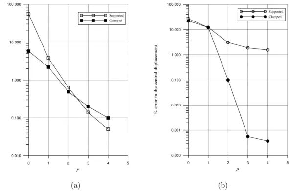
wherew
max is the centre deflection of the plate. Tests were performed using 2boundary elements per side of square plates and per quadrant of circular plates in order to assess the p-convergence rate of the constant up to quartic elements, seldom found in the literature. These plots are shown in fig.12, all obtained with the RBM technique to integrate the singular kernels. Clamped plates result in a system of equations where the contributions of the H matrix are can-celled by the null displacement boundary conditions, while supported plates have the G matrix made null by the zero traction boundary conditions. Because the weakly singular integrals in the G matrix are more easily integrated than the strongly singular ones present in the H matrix, it is common to find slightly better results for clamped plates (for the same mesh).
Latin A m erican Journal of Solids and Structures 12 (2012) 948-979
small when compared to the Reissner model. Furthermore, some confusion about the inherent dif-ferences of these plate models still persist among many researchers, making the selection of reliable results for normalization even more difficult (Wang et al., 2001). In the present case, the values of central displacement are normalized in the following form: 4 3
max
/
w
w
qa
Eh
, where q is the dis-tributed load.0 1 2 3 4 5
p 0.010 0.100 1.000 10.000 100.000 % e rr o r in t h e ce n tr al d is p la ce m en t Supported Clamped
0 1 2 3 4 5
p 0.000 0.001 0.010 0.100 1.000 10.000 100.000 % e rr o r in t h e ce n tr al d is p la ce m en t Supported Clamped
(a) (b)
Figure 12: p-convergence rates for plates under uniform loading. (a) square plate. (b) circular plate.
Figure 13 compares linear, quadratic, cubic and quartic elements of the present implementation with several precursor finite elements now found in commercial software for the maximum normal-ized displacement of a clampled thin square plate obatined with RBM. It is clear why the addtional mathematical complexity of integral equation methods pays off when it comes to accuracy of the results. Similar curves were obtained for boundary forces and moments.
Latin A m erican Journal of Solids and Structures 12 (2015) 948-979
1 2 3 4 5 6 7 8 9 10 11 12
# BE per side
0.900 0.950 1.000 1.050 1.100 1.150 1.200 1.250
w
nLinear BE Quadratic BE Cubic BE Quartic BE
4 noded FE (Hughes et al. [1977]) DKT FE (Batoz et al. [1980]) LR FE (Pugh et al. [1978]) QUAD4* FE (Hinton e Huang [1986]) QUAD9* FE (Hinton e Huang [1986]) 8 noded FE (Voyiadjs e Pecquet [1987]) 4 noded FE (Briassoulis [1992]) Green function (Barbieri [1992])
Figure 13: Comparison of convergence curves for several numerical formulations. Clamped square plate under uniform loading. Solid symbols refer to the present results.
Latin A m erican Journal of Solids and Structures 12 (2012) 948-979
2 3 4 5 6 7 8
0.900 1.000 1.100 1.200 1.300 1.400 1.500 1.600
Rigid body movement
Kutt
Present work
2 3 4 5 6 7 8
0.950 0.975 1.000 1.025 1.050 1.075
Rigid body movement
Kutt
Present work
1 2 3 4 5 6
0.975 1.000 1.025 1.050 1.075
Rigid body movement
Present work
n
w wn
n
w
Number of elements per side
Number of elements per side Number of elements per side
(a) (b)
(c)
w
w
w
Figure 14: Convergence curves for thin square plates under uniform loading using RBM technique, Kutt’s quadrature or the direct method to integrate singular kernels. (a) Constant BE. (b) Linear BE. (c) Quadratic BE.
The present results for SS2-supported square plates under uniform distributed load were normalized against the results of Lee et al. (2002). Figure 15 presents the convergence curves for
h a
/
0.1
Latin A m erican Journal of Solids and Structures 12 (2015) 948-979
h/a
0.05 0.10 0.15 0.20 0.25
Yuan & Miller[yuan88] 0.01417 0.01618 0.01939 0.02371 0.02913 Deshmukh & Archer[des73] 0.01451 0.01643 - 0.02366 - Present Linear (66 mesh) 0.01453 0.01648 0.01957 0.02378 0.02009 Present Quadratic (33 mesh) 0.01451 0.01645 0.01953 0.02373 0.02904
Table 1: Numerical results for clamped square plates under uniform loading.
h/a
0.05 0.10 0.15 0.20 0.25
Yuan & Miller[yuan88] 0.04650 0.05019 0.05480 0.06018 0.06683 Deshmukh & Archer[des73] 0.04677 0.05009 - 0.05900 - Present Linear (66 mesh) 0.04535 0.04882 0.05367 0.05954 0.06631 Present Quadratic (33 mesh) 0.04578 0.04942 0.05432 0.06014 0.06684
Table 2: Numerical results for SS-1 supported square plates under uniform loading.
h/a
0.05 0.10 0.15 0.20
Salerno & Goldberg [1960] (Mindlin) 0.04486 0.04632 0.04676 0.05360 Wang et al. [wang01] (Reissner) 0.04488 0.04630 0.04870 0.05220 Lee et al. [lee01] (Mindlin) 0.04488 0.04663 0.04958 0.05355 Kant & Hinton [kant80] (Higher order model) -- 0.04663 -- 0.05351 Craig [craig87] (Reissner) 0.04492 0.04683 0.05183 0.05353 Katsikadelis & Yotis [kats93] (Reissner) 0.04487 0.04634 -- 0.05221 Long et al.[long88] (Reissner) 0.04458 0.04612 -- 0.05220 Present Linear (66 mesh) 0.04493 0.04668 0.04959 0.05366 Present Quadratic (33 mesh) 0.04497 0.04672 0.04961 0.05368
Table 3: Numerical results for SS2-supported square plates under uniform loading.
The results presented in Tables 1-3 were obtained using RBM technique to integrate the singular kernels. Similar results were obtained for very thick plates using the direct method, presented in Fig.15, and normalized against the analytical results of Lee et al. (2002) for t—e Reissner’s plate model. Therefore we used a shear correction factor 2
5 / 6
, due to the lack of a modern analytical solution for thick Mindlin plates, and a 66 mesh.
Latin A m erican Journal of Solids and Structures 12 (2012) 948-979
Figure 16 shows the shear force along the side of clamped square plate under uniform load, using quadratic elements. It is interesting to note how well the effect is captured in spite of the coarse mesh used.
1 2 3 4 5 6 7 8
0.998 1.000 1.002 1.004 1.006 1.008 1.010
Lee et al. [14] Linear element Quadratic element
1 2 3 4 5 6 7 8
0.990 0.995 1.000 1.005 1.010 1.015 1.020
Lee et al. [14] Linear element Quadratic element
n
w
w
nNumber of elements per side Number of elements per side
(a) (b)
(2002) (2002)
Figure 15. Convergence curves for thick square plates under uniform loading using the direct method to integrate singular kernels. (a) h/a = 0.15. (b) h/a = 0.20.
5.2 Results for Elastic Stability Problems
The performance of the proposed formulation for buckling of supported square plates are presented in Tables 4 (axial compression) and 5 (biaxial compression) and compared with some other refer-ences. These results are presented in the form of buckling coefficient 2
cr
/
N a
D
, where Ncr is the critical compression load. The mesh chosen is 66 constant boundary elements and domain cells. In spite of using only constant elements the results are good.Latin A m erican Journal of Solids and Structures 12 (2015) 948-979
Position along the side of the plate
n
Q
0.00 0.10 0.20 0.30 0.40 0.50
-0.500 -0.400 -0.300 -0.200 -0.100 0.000 0.100
Ratio h/a = 0.05
Figure 16. Shear force along the side of a clamped, uniformly loaded square plate. The continuous line refers do the analytical solution and the symbols to the present results.
h/a
0.001 0.01 0.05 0.1
3D elasticity (Dawe & Roufaeil, 1982) 4.000 - 3.911 3.741 Rayleigh-Ritz (Dawe & Roufaeil, 1982) 4.000 - 3.929 3.731 FE - 9LE (Cheung et al., 1986) - 88 mesh - 4.100 - 3.758 FE - 36LE (Cheung et al., 1986) - 22 mesh - 3.998 - 3.732 BE Present work (66 mesh) 3.9671 3.9646 3.8977 3.7694
Table 4: Numerical results for critical load factor of supported square plates under axial compression. Constant boundary elements and domain cells.
h/a
0.01 0.1
FE - 8LE (Cheung et al., 1986) - 88 mesh 2.030 1.880 FE - 17LE (Cheung et al., 1986) - 33 mesh 2.000 1.870 BE Present work (66 mesh) 1.9841 1.8818
Latin A m erican Journal of Solids and Structures 12 (2012) 948-979
Figure 17. First buckling mode of a clamped square plate under pure shear. Result generated using 66 constant domain cells inside the domain, and 26 constant boundary elements.
5.3 Results for Non-linear Bending Problems
In the results presented in this section, the load and the maximum displacement are normalized with the plate thickness: 4 4
/
R
qa
Eh
andr
u
max/
h
, where a is the lateral dimension of the plate. Most results refer to linear boundary elements (BE1), whereas both constant (DC0) and line-ar (DC1) domain cells were used to discretize the domain.Table 6 compares the present results with some other numerical solutions. Worth to note is the results of Xiao-Yan et al. (1990), a rare BEM large displacement solution for thick plates. The re-sults of the proposed formulation are presented bor both types of supports for completeness sake. Table 7 analyzes the same case with two opposite sides supported and the two others clamped. A load displacement curve obtained for supported square plates is shown in fig.18.
R
0.9158 4.579 6.868 9.158 Rayleigh-Ritz (Azizian & Dawe, 1985) 0.04053 0.1929 0.2750 0.3467 FSM (Azizian & Dawe, 1985) 0.04205 0.1950 0.2776 0.3494 BEM (Xiao-Yan et al., 1990) 0.04090 0.1942 0.2767 0.3489 Present work (SS2) BE1/DC0 0.04200 0.1969 0.2775 0.3464 Present work (SS2) BE1/DC1 0.04199 0.1958 0.2753 0.3425 Present work (SS1) BE1/DC0 0.04428 0.2056 0.2878 0.3573 Present work (SS1) BE1/DC1 0.04426 0.2041 0.2849 0.3534
Latin A m erican Journal of Solids and Structures 12 (2015) 948-979
R
0.9158 4.579 6.868 9.158 Rayleigh-Ritz (Azizian & Dawe, 1985) 0.01915 0.09513 0.1416 0.1867 FSM (Xiao-Yan et al., 1990) 0.01991 0.09883 0.1469 0.1936
BEM [xiao90] 0.01991 0.09840 0.1455 0.1904
Present work BE1/DC0 0.02020 0.1002 0.1488 0.1957 Present work BE1/DC1 0.02020 0.1001 0.1485 0.1952
Table 7: Numerical results for non-linear bending of SS2 square plates under uniform load.
Finally, in order to show results for a subregion case, the plate with step variation in thickness de-picted in Fig.18 was analyzed with 16 quadratic elements and one single domain cell for each subre-gion. The results are compared against a quadratic FE solution (mesh 2020 elements) obtained with a commercial software for the rotations in Fig.19. The agreement is good even considering the use of constant cells.
) (constante 02
0,
h
02 0,
h h0,015
Figure 18. Two subregion non-linear plate bending example under uniform load.
x
0.00 0.50 1.00 1.50 2.00
Position along the longer axis
-50.00 -40.00 -30.00 -20.00 -10.00 0.00 10.00 20.00 30.00 40.00 50.00
Numeric solution - 20 x 20 FE Present work - linear BE / constant DC
h1
h2
h1
h2
Latin A m erican Journal of Solids and Structures 12 (2012) 948-979
6 CONCLUSIONS
The present work presented a compilation of the relevant integral equations for linear and geomet-rically non-linear bending, as well as elastic stability of moderately thick plates. The hypersingular derivative integral equations for the displacement field were presented, including the corresponding convective terms. The equations were solved using the standard BEM procedure, and different inte-gration approaches were discussed and tested. Object oriented implementation issues are comment-ed aiming a simple, extensible, and reusable research platform architecture. Results were obtaincomment-ed for linear and non-linear elastic bending of selected cases of thick plates under transverse loading. From the results presented it is clear that the application of the BEM for linear bending problems leads to exceptionally good results, even for very coarse meshes. The results shown herein cast an interesting set of benchmarks for comparison with similar methods.
This works summarizes more than 15 years of development and application of the boundary element method for the analysis of thick plates. A work which started shy in early 1990s and result-ed in a solid research line for several years. This work later derivresult-ed to other branches of computa-tional mechanics like structural optimization and Green Functions, but most of this achievements would not be reached without the vision and bold scientific talent of Prof. Clóvis S. de Barcellos.
References
Arnold, D.N. & Falk, R.S., (1989). Edge Effects in the Reissner-Mindlin Plate Theory, in: Noor AK, Belytschko T, Simo JC, editors, Analytical and Computational Models of Shells - The Winter Annual Meeting of the ASME, San Francisco, California, December 10--15, pp.71--89.
Azizian, Z. G. & Dawe, D. J., (1985). Geometrically nonlinear analysis of rectangular mindlin plates using the finite strip method, Computers & Structures 21, pp.423--436.
Barbieri, R. & Barcellos, C.S., (1992). A Modified Local Green's Function Technique for the Mindlin's Plate Prob-lem, In: Brebbia, C.A. & Gipson, G.S. (edss), Boundary Elements XIII - Proc. 13th Int. Conf., Tulsa, Comp. Mech. Publ./Elsevier Appl. Science.
de Barcellos, C.S. & Westphal Jr., T., (1992). Reissner/Mindlin's Plate Models and the Boundary Element Method, in: Brebbia CA, Ingber MS, editors, Proc. 7th Conf. on Boundary Element Technology, pp.589--604, Computational Mechanics Publ.
de Barcellos, C.S., Monken e Silva, L.H., (1989). A Boundary Element Formulation for the Mindlin's Plate Model, in: Brebbia CA, Venturini WC, editors, Proc. of the III Int. Conf. On Boundary Element Technology, pp.123--130, Computational Mechanics Publ.
Batoz, J.L., Bathe, K.J. and Ho, L.W., (1980). A Study of Three-Node Triangular Plate Bending Elements, Int. J. Numer. Methods Eng. 15, pp.1771--1812.
Bui, H.D., (1978). Some Remarks about the Formulation of Three-Dimensional Thermoelastoplastic Problems by Integral Equations, Int. J. Solids & Structures 14, pp.935--939.
Chaves, E.W.V., Fernandes, G.R. & Venturini, W.S. (1999), Plate bending boundary element formulation consi-dering variable thickness’, En–ineerin– Analysis wit— Boundary Elements 25, 405 418.