Two efficient hybrid-Trefftz elements for plate bending analysis
Abstract
This study is devoted to the analysis of the Reissner-Mindlin plate bending. In this paper, the hybrid-Trefftz strategy will be utilized. Two novel and efficient elements are formulated in details. They are a Triangular element (THT) and a quadrilateral element (QHT), which have 9 and 12 degrees of freedom, respectively. In this approach, two independent displacement fields are defined; one within the element and the other on the edges of the element. The internal field is selected in such a manner that the governing equation of thick plates could be satisfied. Boundary field is related to the nodal degree of freedoms by the boundary interpolation functions. To calculate these functions, the edges of the ele-ment are assumed to behave like a Timoshenko beam. The high accuracy and efficiency of the proposed elements and absence of the shear locking in these formulations are all proven, using various numerical tests.
Keywords
finite element, hybrid-Trefftz, thick plate, triangular ele-ment, quadrilateral element.
Mohammad Rezaiee-Pajand∗
and Mohammad Karkon
Civil Engineering Department, Ferdowsi Uni-versity of Mashhad – Iran
Received 22 May 2011; In revised form 23 Jul 2011
∗Author email: [email protected]
1 INTRODUCTION
Since the early days of the finite element method era, many elements have been proposed for the analysis of thick plates bending. Some of these elements have been formulated based on Rayleigh-Ritz method, i.e. the orthodox scheme. Routinely, polynomial functions have been used for displacement field in this technique, which do not satisfy the related governing differential equation. In this version of formulation, efficiency of the finite element is increased by enlarging the element’s degrees of freedom [8, 28]. As a result, extending the degrees of freedom leads to more complex elements. It is obvious that not only the analysts would dislike this complexity, but it also adds to the costs of calculation. Between years 1965 to 1975, researchers’ main concern was to achieve high accuracy by complex elements. On this base, numerous elements with various specifications have been developed to analyze thin and thick plates bending. Through these years, the ideas of the multi-field methods, such as the hybrid approach and mixed scheme, emerged and flourished considerably [11, 23].
were developed. Like the Ritz’s process, the hybrid-Trefftz technique is suitable to solve solid mechanic problems. However, dissimilar to the Ritz’s method, the assumed polynomial for the internal field establishes the governing equation of the structure. In other words, homogeneous and particular solution of the governing equation is used to set up the finite element formulation.
The hybrid-Trefftz method was first applied in examining distorted meshes by Jirousek and Leon in 1970s [15]. Because of high accuracy and efficiency, this technique soon caught the attention of other researchers as well. The mentioned approach has been successfully uti-lized in solving plane elasticity problems [9, 32], thin plates [14, 19], Reissner-Mindlin plates [7, 13, 22], shells [24], Helmholtz problem [33], heat conduction [10], contact problems [26], and three-dimensional structures [21]. In 1995, Jirousek and his colleagues presented a fam-ily of quadrilateral hybrid-Trefftz (HT) p-elements for moderately thick plates [16]. These researchers utilized the modified Bessel function of the first kind, and took advantage of the edge shear equilibrium for their derivation.
In hybrid-Trefftz method, weak form of compatibility between elements is achieved by applying independent boundary displacement field and using variational principles. The Main advantage of this formulation is that it allows for the integration on the boundary, which is not only easier than integration on the surface, but also makes it possible to create polygon elements. Advantages of this technique over conventional ways of the finite element procedures are as follows [14, 25]:
1. There is continuity between elements in the hybrid method, and there is no need to establish continuity as an additional condition.
2. It is possible to define numerous degrees of freedom on the boundary for the element, without involving further new and complex formulation.
3. Because of using polynomials, which establish the governing equation, it enjoys high levels of accuracy.
In this study, the edges of the suggested element are designed according to Timoshenko beam, and its deflection and torsion fields are determined. In fact, the boundary interpolation function is considered as a beam component. Interpolation functions for displacement and rotation fields are cubic and quadratic functions, respectively. The boundary field is depended on the nodal displacements by shape functions. By depicting these fields in the general co-ordinates, x-y, the interpolation functions could be acquired. With the use of this boundary field, two new triangular and quadrangular elements are proposed. Accuracy and efficiency of these formulations are proven by utilizing several numerical tests.
2 HYBRID-TREFFTZ FORMULATION
of (u) and boundary displacement of (˜u) are employed independently. The following equation is the hybrid functional of total energy [7, 13]:
Π(u,u˜)=U−W = ∫
πW(u)dΩ
−∫
ΩbiuidΩ
−∫
ΓT
¯
Tiu˜idΓt−∫
ΓTi(ui
−u˜i)dΓ (1)
In this relation, W,bi,Ti, and ˜Tiare strain energy density function, body force, tractions,
and prescribed traction along ΓT, respectively. The strain-energy density function W(u) is
written by W(u)=1/2σijεij. In functional (1), (u) is so selected that the governing equation
would be satisfied. Besides, ˜u provides the continuity and the compatibility between the ele-ments in the weak form. In order to achieve a useful formulation for finite eleele-ments, functional (1) must be stationary in terms of the independent fields, u and ˜u. The process of functional (1) stationary will lead to the following formulas:
δΠ(u,u˜)∣δu=−∫
ΓδTi(ui
−u˜i)dΓ=0 (2)
δΠ(u,u˜)∣δu˜= ∫ Γ
Tiδu˜idΓ−∫
ΓT
¯
Tiδu˜idΓ=0 (3)
It should be added that for utilizing these formulas, ui, ˜ui, and Ti must be specified. In
addition, ui and Ti could be written as the total of two homogeneous and particular parts.
Boundary field of ˜ui could be also associated with nodal displacements by interpolation
func-tions:
{u}={up}+ m ∑ j=1
{φj}cj ={up}+[Φ] {c} (4)
{u˜}=[N˜] {d˜} (5)
{T}={Tp}+[Θ] {c} (6)
In these formulas, {up} is the particular solution of the governing equation, and [Φ] {c}
is its homogeneous solution. Moreover, {d˜} is the nodal displacement and [N˜] is boundary interpolation function. Also, {Tp} represents tractions resulted from {up} and [Θ] {c}
repre-sents tractions resulted from homogeneous solution of the governing equation. By inserting functions (4), (5), and (6) into formulas (2) and (3), the following equations will be available:
δ{c}T[∫
Γ[Θ]
T{
up}dΓ+∫
Γ[Θ]
T[
φ]dΓ{c}−∫
Γ[Θ]
T[˜
N]dΓ {d}]=0 (7)
δ{d}T[∫
Γ[ ˜
N]T{Tp}dΓ+∫
Γ[ ˜
N]T[Θ]dΓ{c}−∫
ΓT
[N˜] {T¯}dΓ]=0 (8)
By finding {c} from the formula (7), and putting it in the equality (8), the succeeding result can be achieved:
In this equation, {h},{g},[H]and [G] are defined in the below form:
{h}= ∫
Γ[Θ]
T{
up}dΓ (10)
{g}= ∫
Γ[ ˜
N]T{Tp}dΓ −∫
ΓT
[N˜]T{T¯} dΓ (11)
[H]= ∫
Γ[Θ]
T
[φ]dΓ (12)
[G]= ∫
Γ[Θ]
T[˜
N]dΓ (13)
Kd=f (14)
Eventually, the stiffness matrix [K] and the nodal forces {f} are obtained, as follows:
[K]=[G]T[H]−1[G] (15)
{f}=[G]T[H]−1{h}−{g} (16)
These formulas are applicable to plane stress, bending plates, and shell problems. In the subsequent sections, the plates bending structures, based on the Reissner-Mindlin theory, will be analyzed.
3 THICK PLATE PROBLEM
One of the most widely-used theories in analyzing thick plates is Reissner-Mindlin hypothesis. This theory utilizes first order shear deformation for analysis. Furthermore, because of using independent displacement and rotation fields, it is only needed to establish compatibility ofC○
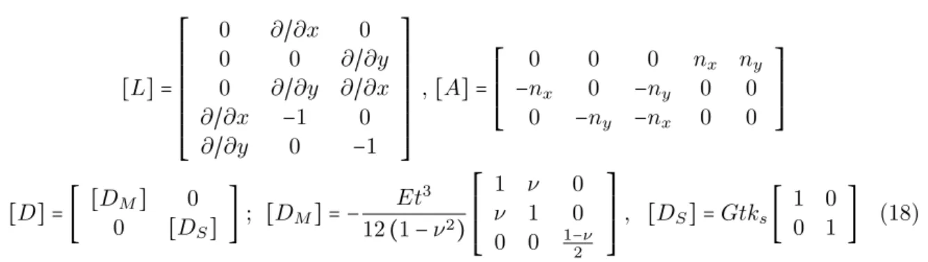
among the elements. Finite element users are aware that establishment of such a connection is by far easier than fulfilling compatibility of C1, which is necessary in Kirchhoff’s theory. Equations of displacement, stress, strain, and the relationship between them, and also tractions in thick plate could be expressed as in the next formulas:
{u}={ w θx θy } T
{ε}={ κx κy κxy γx γy } T
=[L] {u}
{σ}={ Mx My Mxy Qx Qy }
T
=[D] {ε}
{T}={ Qn −Mnx −Mny } T
=[A] {σ} (17)
[L]=
⎡⎢ ⎢⎢ ⎢⎢ ⎢⎢ ⎢⎢ ⎢⎣
0 ∂/∂x 0
0 0 ∂/∂y
0 ∂/∂y ∂/∂x ∂/∂x −1 0
∂/∂y 0 −1
⎤⎥ ⎥⎥ ⎥⎥ ⎥⎥ ⎥⎥ ⎥⎦
,[A]=⎡⎢⎢⎢
⎢⎢ ⎣
0 0 0 nx ny
−nx 0 −ny 0 0
0 −ny −nx 0 0
⎤⎥ ⎥⎥ ⎥⎥ ⎦
[D]=[ [DM] 0
0 [DS] ]
; [DM]=−
Et3
12(1−ν2) ⎡⎢ ⎢⎢ ⎢⎢ ⎣
1 ν 0
ν 1 0 0 0 1−ν
2 ⎤⎥ ⎥⎥ ⎥⎥ ⎦
, [DS]=Gtks[
1 0
0 1 ] (18)
In these equations, ks is shear correction factor, which is usually, assumed 5/6. The
direction cosines of the element’s side, in thex and y directions, arenx and ny, respectively:
{ nx=cosα= y2 −y1 l21 =
y21
l21
ny=sinα=−x2 −x1 l21 =
x21
l21
(19)
Figure 1 Boundary forces on an arbitrary direction.
The static equilibrium equation for plates is given below:
[L]T{σ}=[L]T[D] [L] {u}=−{P} (20)
The vector{P} in the present formula, is actually the vector of external loads entering the plate, and is defined as follows:
{P}={ p 0 0 }T (21)
By inserting the formula (21) into the equation (20) and simplifying it, the governing equations of thick plate are obtained in the following appearance [22]:
∇4w= p D−
1
ksGt
( t2
12ks∇ 2
−1) (∂p
∂x−D∇
4
θx)=0
( t2
12ks∇ 2
−1) (∂p
∂y−D∇
4
θy)=0
Present formulas are based on the Reissner-Mindlin theory. The solution of the homoge-neous part of the differential equation (22), which is independent of loading, could be found by solving the bi-harmonic one,∇4wc=0. After solving the last equation in polar coordinates,
the homogeneous solution is obtained in the below shape [12]:
wc= ∞ ∑ n=0
[anrncosnθ+bnrnsinnθ+cnrn +1
cos(n−1)θ+dnrn +1
sin(n−1)θ] (23)
It is suitable to utilize the following complex variables:
z=reiθ=r[cos(θ)+isin(θ)]
zn=(reiθ)n=rn[cos(nθ)+isin(nθ)]
(24)
Substituting these equations into (23) leads to the below solution [25]:
wc= ∞ ∑ n=0
{Re[(an+r
2
bn)zn]+Im[(cn+r
2
dn)zn]}
r2=x2+y2, z=x+iy
(25)
Therefore, the values ofwj are accessible by applying the equations below. These formulas
were first introduced by Herrera [12].
⎧⎪⎪⎪⎪ ⎪⎪ ⎨⎪⎪⎪ ⎪⎪⎪⎩
w4k=r 2
Re(zk) w4k+1=r
2
Im(zk) w4k+2=Re(zk
+2 )
w4k+3=Im(zk
+2 )
k=0,1,2, . . . (26)
The first eleven terms of the expression can be found by using k=0,1,2. As a result, the succeeding solutions are obtained:
k=0⎧⎪⎪⎪⎪⎪⎪⎨⎪⎪⎪ ⎪⎪⎪⎩
w0=0
w1=x 2
+y2 w2=2xy
w3=x 2
−y2
; k=1 ⎧⎪⎪⎪⎪⎪⎪⎨⎪⎪⎪ ⎪⎪⎪⎩
w4=x 3
+xy2 w5=x
2
y+y3 w6=3x
2
y−y3 w7=x
3
+3xy2
; k=2⎧⎪⎪⎪⎪⎪⎪⎨⎪⎪⎪ ⎪⎪⎪⎩
w8=x 4
+y4 w9=2x
3
y+2xy3 w10=x
4
−6x2y2+y4 w11=4x
3
y−4xy3
(27)
wp= pr2
64D(r
2
− 16D
Gtks)
(28)
To find the homogeneous solution for the equation (3), Petrolito supposed θx and θyin the
following manner [22]:
θx= ∂w ∂y +
D Gtks
f1(x, y)
θy=− ∂w ∂x −
D Gtks
f2(x, y)
(29)
The unknown functions, f1 and f2, are obtained by inserting the present relationships in the governing equation (3). Therefore, the homogeneous solution of equation (3) could be expressed as in below:
θx= ∂w ∂y + D Gtks ∂ ∂y∇ 2 w
θy=−∂w
∂x − D Gtks ∂ ∂x∇ 2 w (30)
It is obvious that the internal rotation functions, θx and θy, are dependent on the
deflec-tion w. Consequently, the field function of particular solution is accessible in the following appearance:
{up}=⎧⎪⎪⎪⎨⎪⎪⎪
⎩ wp θxp θyp ⎫⎪⎪⎪ ⎬⎪⎪⎪ ⎭ =⎧⎪⎪⎪⎪⎪⎨ ⎪⎪⎪⎪⎪ ⎩ pr2
64D(r 2
− 16D
Gtks) yr2p
16D
−xr2p
16D ⎫⎪⎪⎪⎪ ⎪⎬ ⎪⎪⎪⎪⎪ ⎭ (31)
In the particular and homogeneous solution, there is no advantage over x and y, and therefore, the element will be rotational invariant.
The minimum of terms which are selected from homogeneous solution depends on the element’s degrees of freedom. Number of necessary terms (and not adequate) to prevent numerical instability and deficiency of the rank of the stiffness matrix is acquired through the next condition [14, 25]:
m≥n−r (32)
direction of the x-axis andy-axis. Taking these points in consideration, the formula (32) for the plate changes to the following form:
m≥N DOF−3 (33)
It was stated that use of the minimum number (m=n-r) of the Trefftz functions in Eq. (4) does not always guarantee a stiffness matrix with full rank. Moreover, the full rank may always be achieved by suitably augmenting m. The optimal value of m for a given type of element should be found by numerical experimentation [25].
4 BOUNDARY DISPLACEMENT FIELD
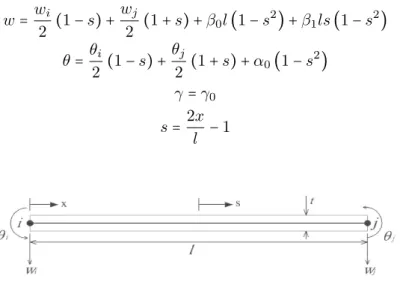
The boundary displacement functions are related to the nodal degrees of freedom by shape functions. In order to find boundary shape functions, the edges of the element are assumed to behave like a Timoshenko beam. This beam element was utilized by other researchers for plate bending analysis [6, 29, 30, 35]. The shape functions of the Timoshenko beam are calculated based on Figure 2. Linear field is also used for torsion of this beam. In order to compute shape function of the beam in Figure 2, a cubic displacement polynomial and a quadratic rotational field are selected. Moreover, it is assumed that shear strain has the constant value ofγ0. Based on these assumptions, the following equations can be written:
w= wi
2 (1−s)+
wj
2 (1+s)+β0l(1−s 2
)+β1ls(1−s 2
)
θ= θi
2 (1−s)+
θj
2 (1+s)+α0(1−s 2
)
γ=γ0
s= 2x
l −1 (34)
Figure 2 Timoshenko beam.
γ = dw dx −θ=
2
l ⋅ dw
ds −θ
γ0= 2
l (− wi
2 +
wj
2 −2β0ls+β1l−3β1ls 2
)−θi(
1−s
2 )−θj( 1+s
2 )−α0(1−s 2
) (35)
In the present formula, coefficients of the terms s ands2
are equivalent to zero. Therefore, in the succeeding lines, α0,β1 are determined in terms of the unknown parameterγ0:
Γ=2
l (wj−wi)−(θi+θj)
β0= 1
8(θi−θj)
α0=− 3 2(γ0−
1 2Γ)
β1= 1
6α0 (36)
At this stage, there is only one unknown constant γ0, which can be determined from the condition of minimum strain energy. It should be added that the structural strain energy is the sum of bending and shear strain energy. Bending strain energy is calculated in the following way:
Ub= D
2 ∫
l
0
κ2dx= Dl
4 ∫ 1
−1
κ2ds
D= Et
3
12(1−ν2) (37)
In this equation, κ represents curvature and is determined below:
κ=−2
l ⋅ dθ
ds =κ0−6 sγ0
l
κ0= 1
l (θi−θj+3sΓ) (38)
Substituting these equations into (37) leads to the below bending strain energy:
Ub=U0+6(−
DΓγ0
l + Dγ02
l )
U0=
Dl
4 ∫ 1
−1κ 2
Besides, the next equation determines the energy of shear strain:
Us= C
2 ∫
l
0 γ dx=
Cl
4 ∫ 1
−1γ 0ds=
Cl
2 γ 2 0
C=Gtks (40)
By adding the bending and shear strain energy together, total strain energy is found, as follows:
U =Ub+Us=U0− 6DΓ
l γ0+
6D l γ 2 0+ Cl 2 γ 2 0 (41)
Implementing ∂U/∂γ0=0 will give the following results:
γ0=
6DΓ
Cl2+12D =δΓ
δ= 6λ
1+12λ , λ= D
Cl2 (42)
By substitution β1, β0, α0 andγ0into (34), the succeeding shape functions for Timoshenko beam can be found:
{ wθ˜˜
n }=[ N1 N5 N2 N6 N3 N7 N4
N8 ] ⎧⎪⎪⎪⎪ ⎪⎪ ⎨⎪⎪⎪ ⎪⎪⎪⎩ wi θni wj θnj ⎫⎪⎪⎪⎪ ⎪⎪ ⎬⎪⎪⎪ ⎪⎪⎪⎭ (43)
N1= 1 4[2+s
3
(1−2δ)+s(−3+2δ)]
N2=
l
4[0.5(1−s 2
)+(s3−s) (0.5−δ)]
N3= 1 4[2−s
3
(1−2δ)−s(−3+2δ)]
N4=
l
4[−0.5(1−s 2
)+(s3−s) (0.5−δ)]
N5= 1
4l[6(1−s
2
) (−1+2δ)]
N6= 1
4[−1+s(−2+3s)+6(1−s 2
)δ]
N7= 1
4l[−6(1−s
2
) (−1+2δ)]
N8= 1
4[−1+s(2+3s)+6(1−s 2
By assuming a linear interpolation for torsion field, the next results will be in hand:
˜
θs=
1
2(1−s)θs1+ 1
2(1+s)θs2 (45)
{ N1′=(1−s) /2
N′
2=(1+s) /2
(46)
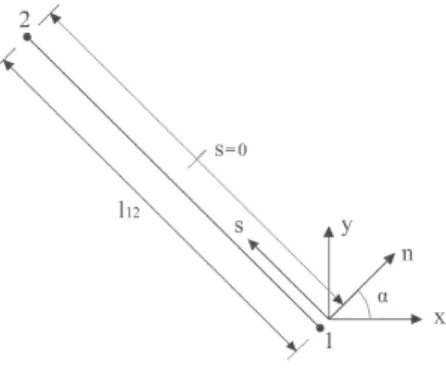
By transferring these fields to the general coordinates, x-y, the shape functions for the element in Figure (3-2) can be written in the following form:
⎧⎪⎪⎪⎪ ⎪⎪ ⎨⎪⎪⎪ ⎪⎪⎪⎩
x21=x2−x1
y21=y2−y1
x=x1+(s+1)x21/2
y=y1+(s+1)y21/2
(47)
Figure 4 leads to the subsequent equations:
{ cosα=y21/l21 sinα=−x21/l21
(48)
Figure 3 Degrees of freedom on the element’s side.
Consequently, the next relationship can be written: ⎧⎪⎪⎪⎪
⎪⎪ ⎨⎪⎪⎪ ⎪⎪⎪⎩
θn1=θx1cosα+θy1sinα
θs1=θy1cosα−θx1sinα
θn2=θx2cosα+θy2sinα
θs2=θy2cosα−θx2sinα
(49)
Furthermore, the boundary field’s ˜θx and ˜θy have the following equations:
{ θ˜x=θ˜ncosα−θ˜ssinα
˜
θy=θ˜nsinα+θ˜scosα
Figure 4 Position of axes on the side.
Boundary displacement field is determined by multiplying shape functions in the nodal displacements, as follows:
{u˜}=[N˜] {d˜} (51)
⎧⎪⎪⎪ ⎨⎪⎪⎪ ⎩
˜
w
˜
θx
˜
θy
⎫⎪⎪⎪ ⎬⎪⎪⎪ ⎭=
⎡⎢ ⎢⎢ ⎢⎢ ⎣
N11 N12 N13 N14 N15 N16
N21 N22 N23 N24 N25 N26
N31 N32 N33 N34 N35 N36 ⎤⎥ ⎥⎥ ⎥⎥ ⎦
⎧⎪⎪⎪⎪ ⎪⎪⎪⎪⎪ ⎪⎪ ⎨⎪⎪⎪ ⎪⎪⎪⎪⎪ ⎪⎪⎪⎩
˜
w1 ˜
θx1 ˜
θy1 ˜
w2 ˜
θx2 ˜
θy2 ⎫⎪⎪⎪⎪ ⎪⎪⎪⎪⎪ ⎪⎪ ⎬⎪⎪⎪ ⎪⎪⎪⎪⎪ ⎪⎪⎪⎭
(52)
All entries of the shape function matrix are presented in the appendix one.
5 NUMERICAL TESTS
The performance of the proposed elements will be assessed in this section. To evaluate the accuracy, convergence rate, and robustness of the new formulation several plate problems will be solved. In order to demonstrate the properties of the proposed elements in details, the results of THT and QHT, will be compared to the following famous elements:
1. The triangular element of Kirchhoff’s discrete plate (DKT) [3].
2. The triangular element of Mindlin’s discrete plate (DKMT) [18].
3. The triangular element according to Reissner-Mindlin’s theory (ARS-T9) [31].
4. The triangular 3-node element with 9 DOF (T3BL) [34].
5. The triangular element with reduced integration (T3BL(R)) [34].
6. The triangular element according to Mindlin’s theory (RDKTM) [6].
8. The quadrilateral element of Mindlin’s discrete plate (DKMQ) [17].
9. The quadrilateral element with reduced integration (Q4BL) [36].
10. Bathe-Dvorkin quadrilateral element (MITC4) [2].
11. The quadrilateral element for Reissner-Mindlin’s plates (ARS-Q12) [30].
12. The quadrilateral 4-node element (AC-MQ4) [5].
5.1 Study of Trefftz function effect
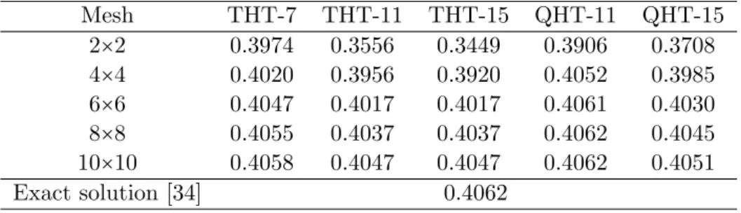
In this part, the number of Trefftz functions will be examined carefully through various nu-merical examples in view of accuracy and efficiency of computation. For this purpose, a square plate with simply support is solved under a uniformly distributed load q. The obtained solu-tions confirm a typical pattern of accuracy when the number of function terms will increase. To demonstrate the effect of Trefftz function terms, the integer n represents the number of the used terms, in THT-n and QHT-n. Table 1 reveals the minimum number of Trefftz function terms, which are sufficient for present formulation, and compatible with the necessary condi-tion of Eq. (33). The findings of this study show that the triangular element THT with 7 Trefftz functions and the quadrangular element QHT with 11 Trefftz functions have the highest level of accuracy for plate analysis.
Table 1 Accuracy test for varying Trefftz terms in simply support plate (Wc/ (qa4/100D)).
Mesh THT-7 THT-11 THT-15 QHT-11 QHT-15
2×2 0.3974 0.3556 0.3449 0.3906 0.3708
4×4 0.4020 0.3956 0.3920 0.4052 0.3985
6×6 0.4047 0.4017 0.4017 0.4061 0.4030
8×8 0.4055 0.4037 0.4037 0.4062 0.4045
10×10 0.4058 0.4047 0.4047 0.4062 0.4051
Exact solution [34] 0.4062
5.2 Analysis of square plate
Furthermore, the suggested elements are insensitive to mesh distortion. The comparisons of the present results with those obtained by other authors are also presented in Tables 10 to 13.
Table 2 Central deflections for the simply supported square plate (Wc/ (ql4/100D)).
Mesh 0.001=h/l
ARS-T9 T3BL Q4BL MITC4 ARS-Q12 AC-MQ4 THT QHT
2×2 0.3676 0.3798 0.4035 0.3969 0.4045 0.4052 0.4019 0.4052 4×4 0.3973 0.4005 0.4058 0.4041 0.4060 0.4062 0.4055 0.4062 8×8 0.4041 0.4054 0.4062 0.4057 0.4062 0.4062 0.4061 0.4062 16×16 0.4057 0.4063 0.4062 0.4061 0.4062 0.4062 0.4062 0.4062
Exact solution [34] 0.4062
Table 3 Central deflections for the simply supported square plate (Wc/ (ql4/100D)).
Mesh 0.1=h/l
ARS-T9 T3BL Q4BL MITC4 ARS-Q12 AC-MQ4 THT QHT
2×2 0.3845 0.4036 0.4269 0.4190 0.4228 0.4139 0.4218 0.4265 4×4 0.4165 0.4212 0.4274 0.4255 0.4255 0.4206 0.4257 0.4266 8×8 0.4245 0.4257 0.4273 0.4268 0.4267 0.4251 0.4268 0.4270 16×16 0.4266 0.4269 0.4273 0.4272 0.4271 0.4267 0.4271 0.4272
Exact solution [34] 0.4273
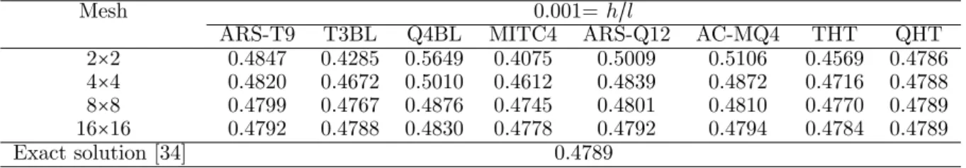
Table 4 Central moments for the simply supported square plate (Mc/ (ql2/10)).
Mesh 0.001=h/l
ARS-T9 T3BL Q4BL MITC4 ARS-Q12 AC-MQ4 THT QHT
2×2 0.4847 0.4285 0.5649 0.4075 0.5009 0.5106 0.4569 0.4786 4×4 0.4820 0.4672 0.5010 0.4612 0.4839 0.4872 0.4716 0.4788 8×8 0.4799 0.4767 0.4876 0.4745 0.4801 0.4810 0.4770 0.4789 16×16 0.4792 0.4788 0.4830 0.4778 0.4792 0.4794 0.4784 0.4789
Exact solution [34] 0.4789
Table 5 Central moments for the simply supported square plate (Mc/ (ql2/10)).
Mesh 0.1=h/l
ARS-T9 T3BL Q4BL MITC4 ARS-Q12 AC-MQ4 THT QHT
2×2 0.4765 0.4484 0.4716 0.4075 0.5223 0.5025 0.4923 0.4729 4×4 0.4775 0.4744 0.4773 0.4612 0.4941 0.4842 0.4872 0.4766 8×8 0.4781 0.4785 0.4785 0.4745 0.4834 0.4803 0.4814 0.4783 16×16 0.4786 0.4789 0.4788 0.4778 0.4801 0.4792 0.4795 0.4787
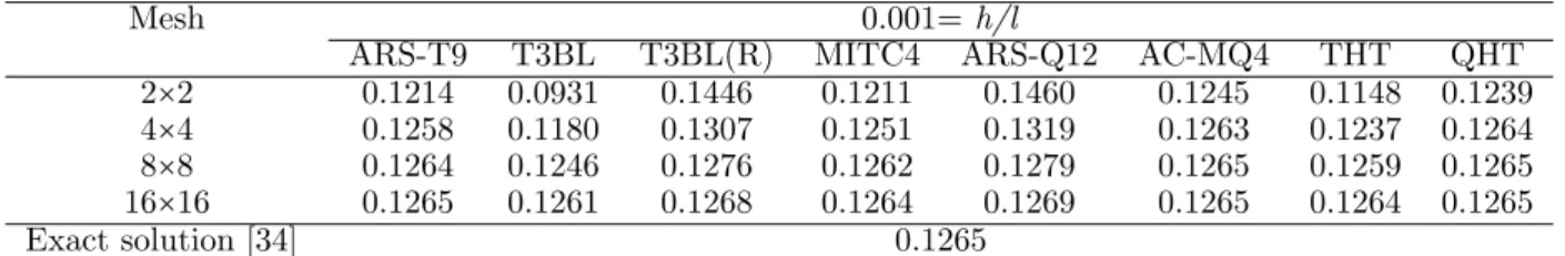
Table 6 Central deflections for the clamped supported square plate (Wc/ (ql4/100D)).
Mesh 0.001=h/l
ARS-T9 T3BL T3BL(R) MITC4 ARS-Q12 AC-MQ4 THT QHT
2×2 0.1214 0.0931 0.1446 0.1211 0.1460 0.1245 0.1148 0.1239
4×4 0.1258 0.1180 0.1307 0.1251 0.1319 0.1263 0.1237 0.1264
8×8 0.1264 0.1246 0.1276 0.1262 0.1279 0.1265 0.1259 0.1265
16×16 0.1265 0.1261 0.1268 0.1264 0.1269 0.1265 0.1264 0.1265
Exact solution [34] 0.1265
Table 7 Central deflections for the clamped supported square plate (Wc/ (ql4/100D)).
Mesh 0.1=h/l
ARS-T9 T3BL T3BL(R) MITC4 ARS-Q12 AC-MQ4 THT QHT
2×2 0.1392 0.1263 0.1691 0.1431 0.1678 0.1474 0.1367 0.1504
4×4 0.1473 0.1450 0.1552 0.1488 0.1548 0.1477 0.1470 0.1507
8×8 0.1495 0.1491 0.1516 0.1500 0.1515 0.1494 0.1494 0.1505
16×16 0.1502 0.1501 0.1508 0.1504 0.1507 0.1502 0.1502 0.1505
Exact solution [34] 0.1505
Table 8 Central moments for the clamped supported square plate (Mc/ (ql2/10)).
Mesh 0.001=h/l
ARS-T9 T3BL T3BL(R) MITC4 AC-MQ4 THT QHT
2×2 0.2473 0.1408 0.1617 0.1890 0.2712 0.2391 0.2211 4×4 0.2347 0.2102 0.2122 0.2196 0.2407 0.2276 0.2284 8×8 0.2302 0.2248 0.2249 0.2267 0.2321 0.2284 0.2290 16×16 0.2293 0.2280 0.2280 0.2285 0.2298 0.2289 0.2291
Exact solution [34] 0.2291
Table 9 Central moments for the clamped supported square plate (Mc/ (ql2/10)).
Mesh ARS-T9 T3BL T3BL(R) 0.1=MITC4h/l AC-MQ4 THT QHT
2×2 0.2388 0.1596 0.1647 0.1898 0.2572 0.2424 0.2271 4×4 0.2313 0.2150 0.2155 0.2219 0.2377 0.2372 0.2310 8×8 0.2311 0.2277 0.2279 0.2295 0.2333 0.2335 0.2317 16×16 0.2317 0.2309 0.2310 0.2314 0.2323 0.2324 0.2319
Exact solution [34] 0.2310
Table 10 Central deflections for the simply supported square plate (Wc/ (ql4/100D)).
h/l Mesh type Element type 2×2 4×4 8×8 16×16 Exact solution [34]
10−20
A
ARS-T9 0.3676 0.3973 .04041 0.4057
0.4062 ARS-Q12 0.4045 0.4060 0.4062 0.4062
THT 0.4019 0.4055 0.4061 0.4062 QHT 0.4052 0.4062 0.4062 0.4062
B
ARS-T9 0.3771 0.3994 0.4046 0.4058 ARS-Q12 0.4218 0.4102 0.4072 0.4065 THT 0.4010 0.4053 0.4060 0.4062 QHT .04037 0.4061 0.4062 0.4062
C
ARS-T9 0.3802 0.4003 0.4048 0.4059 ARS-Q12 0.4324 0.4131 0.4080 0.4067 THT 0.3993 0.4048 0.4059 0.4062 QHT 0.4020 0.4059 0.4062 0.4062
Table 11 Central deflections for the simply supported square plate (Wc/ (ql4/100D)).
h/l Mesh type Element type 2×2 4×4 8×8 16×16 Exact solution [34]
0.2
A
ARS-T9 0.4370 0.4764 0.4867 0.4895
0.4904 ARS-Q12 0.4857 0.4859 0.4900 0.4903
THT 0.4804 0.4876 0.4897 .0.4902 QHT 0.4901 0.4900 0.4903 0.4904
B
ARS-T9 0.4592 0.4804 0.4878 0.4897 ARS-Q12 0.5003 0.4922 0.4908 .4905
THT 0.4780 0.4863 0.4892 0.4901 QHT 0.4887 0.4895 .4901 0.4904
C
Table 12 Central deflections for the clamped supported square plate (Wc/ (ql /100D)).
h/l Mesh type Element type 2×2 4×4 8×8 16×16 Exact solution [34]
10−20
A
ARS-T9 0.1214 0.1258 0.1264 0.1265
0.1265 ARS-Q12 0.1460 0.1319 0.1279 0.1269
THT 0.1148 0.1237 0.1259 0.1264 QHT 0.1239 0.1260 0.1265 0.1265
B
ARS-T9 0.1361 0.1291 0.1272 0.1267 ARS-Q12 0.1601 0.1354 0.1288 0.1271 THT 0.1141 0.1229 0.1256 0.1263 QHT 0.1235 0.1259 0.1264 0.1265
C
ARS-T9 0.1443 0.1311 0.1276 0.1268 ARS-Q12 0.1700 0.1383 0.1295 0.1273 THT 0.1163 0.1231 0.1256 0.1263 QHT 0.1238 0.1260 0.1264 0.1265
Table 13 Central deflections for the clamped supported square plate (Wc/ (ql4/100D)).
h/l Mesh type Element type 2×2 4×4 8×8 16×16 Exact solution [34]
0.2
A
ARS-T9 0.1931 0.2101 0.2152 0.2167
0.2167 ARS-Q12 0.2348 0.2217 0.2183 0.2175
THT 0.1971 0.2120 0.2158 0.2169 QHT 0.2216 0.2183 0.2175 0.2173
B
ARS-T9 0.2145 0.2160 0.2168 0.2171 ARS-Q12 0.2494 0.2253 0.2192 0.2177 THT 0.1930 0.2104 0.2154 0.2167 QHT 0.2201 0.2181 0.2174 0.21473
C
ARS-T9 0.2265 0.2191 0.2176 0.2173 ARS-Q12 0.2598 0.2281 0.2199 0.2179 THT 0.2001 0.2119 0.2158 0.2168 QHT 0.2196 0.2180 0.2174 0.2173
5.3 Circular plate test
Figure 6 Three mesh types for quadrant of a circular plate.
Table 14 Central deflections for the simply supported circular plate (Wc/ (qa4/10D)).
Number of elements ARS-T9 T3BL DKMT DKMQ0.02=MITC4h/a ARS-Q12 THT QHT
3 0.6056 0.6306 0.6056 0.6101 0.5829 0.6101 0.6548 0.6521
12 0.6306 0.6345 0.6304 0.6309 0.6246 0.6308 0.6420 0.6414
48 0.6367 0.6366 0.6357 0.6357 0.6342 0.6357 0.6385 0.6384
Exact solution [34] 0.6373
Table 15 Central deflections for the simply supported circular plate (Wc/ (qa4/10D)).
Number of elements 0.2=h/a
ARS-T9 T3BL DKMT DKMQ MITC4 ARS-Q12 THT QHT
3 0.6314 0.6586 0.6314 0.6346 0.6101 0.6353 0.6813 0.6791
12 0.6575 0.6629 0.6575 0.6576 0.6524 0.6575 0.6695 0.6688
48 0.6650 0.6649 0.6636 0.6635 0.6623 0.6635 0.6665 0.6663
Exact solution [34] 0.6656
Table 16 Central moments for the simply supported circular plate (Mc/ (qa2/10)).
Number of elements ARS-T9 T3BL DKMT DKMQ0.02=MITC4h/a ARS-Q12 THT QHT
3 0.2105 0.1883 0.2104 0.2156 0.1892 0.2156 0.2100 0.2104
12 0.2095 0.2012 0.2092 0.2080 0.2040 0.2081 0.2079 0.2073
48 0.2078 0.2050 0.2072 0.2068 0.2056 0.2069 0.2067 0.2065
Exact solution [34] 0.2063
Table 17 Central deflections for the clamped supported circular plate (Wc/ (qa4/10D)).
Number of elements ARS-T9 T3BL DKMT DKMQ0.02=MITC4h/a ARS-Q12 THT QHT
3 0.1649 0.0968 0.1649 0.1723 0.1451 0.1723 0.1272 0.1244
12 0.1598 0.1404 0.1599 0.1615 0.1552 0.1613 0.1491 0.1485
48 0.1575 0.1524 0.1576 0.1578 0.1563 0.1577 0.1547 0.1545
Table 18 Central deflections for the clamped supported circular plate (Wc/ (qa /10D)).
Number of elements ARS-T9 T3BL DKMT DKMQ0.2=MITC4h/a ARS-Q12 THT QHT
3 0.1907 0.1286 0.1907 0.1968 0.1721 0.1975 0.1536 0.1514
12 0.1870 0.1696 0.1872 0.1882 0.1829 0.1881 0.1765 0.1759
48 0.1854 0.1808 0.1855 0.1856 0.1844 0.1856 0.1827 0.1825
Exact solution [34] 0.1848
Table 19 Central moments for the simply supported circular plate (Mc/ (qa2/10)).
Number of elements ARS-T9 T3BL DKMT DKMQ0.02=MITC4h/a ARS-Q12 THT QHT
3 09602 0.4875 0.9600 1.0160 0.7520 1.0183 0.7250 0.7317
12 0.8715 0.7275 0.8680 0.8600 0.8200 0.8600 0.7969 0.7909
48 0.8324 0.7909 0.8280 0.8240 0.8160 0.8260 0.8089 0.8069
Exact solution [34] 0.8125
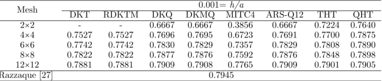
5.4 Razzaque skew plate
Figure 7 shows a 60○
skew plate which was originally studied by Razzaque [27]. This plate has simply supported on two opposite edges and free on the other two edges, and subjected to a uniformly distributed load. The results obtained using the THT and QHT elements, are shown in Tables 20 and 21. The referenced value was obtained by Razzaque with 16×16 finite
difference mesh.
Figure 7 Razzaque skew plate with mesh (4×4).
Table 20 Central deflections for Razzaque skew plate (Wc/ (qa4/100D)).
Mesh 0.001=h/a
DKT RDKTM DKQ DKMQ MITC4 ARS-Q12 THT QHT
2×2 - - 0.6667 0.6667 0.3856 0.6667 0.7224 0.7640
4×4 0.7527 0.7527 0.7696 0.7695 0.6723 0.7691 0.7700 0.7875 6×6 0.7742 0.7742 0.7830 0.7829 0.7357 0.7829 0.7808 0.7890 8×8 0.7822 0.7822 0.7877 0.7876 0.7592 0.7876 0.7848 0.7898 12×12 0.7881 0.7881 0.7909 0.7908 0.7765 0.7909 0.7901 0.7905
Table 21 Central moments for Razzaque skew plate (My/ (qa2/10)).
Mesh DKMQ MITC40.001=ARS-Q12h/a THT QHT
2×2 0.9220 0.4688 0.9246 0.8587 0.7521 4×4 0.9600 0.8256 0.9595 0.9457 0.9504 6×6 0.9610 0.8976 0.9609 0.9521 0.9416 8×8 0.9610 0.9242 0.9605 0.9553 0.9481 12×12 0.9600 0.9439 0.9602 0.9577 0.9545
Razzaque [27] 0.9589
5.5 Morley skew plate
The simply supported skew plate illustrated in Figure (8) has been solved by Morley. This researcher used polar co-ordinates and a least-squares solution procedure to analyze an acute skew plate subject to a uniformly distributed load. It is worth emphasizing that this problem poses severe difficulties for numerical methods, since there is a singularity in the bending moments at the obtuse corner. Despite these difficulties, in the case of the thin-plate theory, Morley’s solution is assumed to be near exact. Babuka and Scapolla also solved this problem as a 3-D elastic structure. The results were obtained using suggested elements, and compared to some other famous formulations, as shown in Tables (22) through (24) and Figure (9).
Figure 8 Morley skew plate with mesh (4×4).
Table 22 Central deflection for the Morley skew plate (Wc/ (qa4/1000D)).
Mesh T3BL Q4BL MITC4 DKMQ0.001=ARS-Q12h/a AC-MQ4 THT QHT
2×2 0.421 0.512 0. 358 0.760 0.756 0.431 0.423 0.422
4×4 0.415 0.439 0.343 0.507 0.506 0.409 0.406 0.409
8×8 0.414 0.429 0.343 0.443 0.442 0.405 0.406 0.408
16×16 0.413 0.424 0.362 0.425 0.424 0.405 0.407 0.408
Table 23 Central deflection for the Morley skew plate (Wc/ (qa /1000D)).
Mesh T3BL Q4BL MITC4 DKMQ0.01=ARS-Q12h/a AC-MQ4 THT QHT
2×2 0.422 0.513 0. 359 0.757 0.754 0.431 0.424 0.425
4×4 0.417 0.440 0.357 0.504 0.503 0.410 0.408 0.413
8×8 0.418 0.431 0.383 0.441 0.440 0.407 0.410 0.414
16×16 0.420 0.427 0.404 0.423 0.423 0.409 0.413 0.416
References Morley solution [20] 0.408
Babuˇska and Scapolla [1] 0.423
Table 24 Maximum central moments for the Morley skew plate (Mmax/ (qa2/10)).
Mesh T3BL Q4BL MITC4 DKMQ0.001=ARS-Q12h/a AC-MQ4 THT QHT
2×2 1.723 2.012 1.669 2.339 2.314 2.142 2.057 1.872
4×4 1.893 1.990 1.733 2.074 2.069 2.001 1.818 1.879
8×8 1.912 1.967 1.717 1.984 1.985 1.928 1.898 1.903
16×16 1.918 1.953 1.777 1.950 1.950 1.903 1.902 1.905
Exact solution [20] 1.910
Table 25 Minimum central moments for the Morley skew plate (Mmin/ (qa2/10)).
Mesh T3BL Q4BL MITC4 DKMQ0.001=ARS-Q12h/a AC-MQ4 THT QHT
2×2 0.955 1.133 0.921 1.751 1.730 1.374 0.976 1.018
4×4 1.090 1.164 0.957 1.276 1.271 1.284 0.918 0.979
8×8 1.100 1.152 0.874 1.166 1.168 1.147 1.056 1.075
16×16 1.100 1.140 0.923 1.137 1.136 1.085 1.074 1.083
Exact solution [20] 1.080
(a) Displacement at centre (b) Bending momentMmaxat centre (c) Bending momentMminat centre
6 CONCLUSION
In this study, the triangular element THT and the quadrangular element QHT are proposed for the analysis of the thick bending plates. Formulations of these elements are based on the hybrid-Trefftz method. The two displacement fields, one within the element and the other on the borders of the element, are supposed to be independent. The independent internal field is defined by utilizing the Trefftz scheme. By assuming that the element’s edges are Timoshenko beam, the required interpolation functions and the boundary displacement field for this beam component are calculated. In order to examine the accuracy and efficiency of the proposed elements, several numerical tests were conducted. As it was proven by the numerical results, the answers of the suggested elements quickly converged in all the tests. The present formulations lead to good answers, even when the coarse meshes are utilized. It should be added that the accuracy and convergence rate of the element QHT is higher than the element THT.
References
[1] I. Babuˇska and T. Scapolla. Benchmark computation and performance evaluation for a rhombic plate bending problem.Int. J. Num. Meth. Eng., 28:155–179, 1989.
[2] K.J. Bathe and E.H. Dvorkin. A four-node plate bending element based on Mindlin/Reissner plate theory and mixed interpolation.Int. J. Num. Meth. Eng., 21:367–383, 1985.
[3] J.L. Batoz, K.J. Bathe, and L.W. Ho. A study of three-node triangular plate bending element. Int. J. Num. Meth. Eng., 15:1771–1812, 1980.
[4] J.L. Batoz and M.B. Tahar. Evaluation of a new quadrilateral thin plate bending element. Int. J. Numer. Meth. Eng., 18:1655–1677, 1982.
[5] S. Cen, Y.Q. Long, Z.H. Yao, and S.P. Chiew. Application of the quadrilateral area co-ordinate method: A new element for Mindlin–Reissner plate.Int. J. Numer. Meth. Eng., 66:1–45, 2006.
[6] W. Chen and Y.K. Cheung. Refined 9-Dof triangular mindlin plate elements.Int. J.Num. Meth. Eng., 51:1259–1281, 2001.
[7] Y.S. Choo, N. Choi, and B.C. Lee. A new hybrid-Trefftz triangular and quadrilateral plate elements. Applied Mathematical Modeling, 34:14–23, 2010.
[8] H.R. Dhananjaya, J. Nagabhushanam, P.C. Pandey, and Zamin Jumaat Mohd. New twelve node serendipity quadri-lateral plate bending element based on mindlin-reissner theory using integrated force method.Structural Engineering and Mechanics, 36(5):625–642, 2010.
[9] M. Dhanasekar, J.J. Han, and Q.H. Qin. A hybrid-Trefftz element containing an elliptic hole. Finite Elements in Analysis and Design, 42:1314–1323, 2006.
[10] Z.J. Fu, Q.H. Qin, and W. Chen. Hybrid-Trefftz finite element method for heat conduction in nonlinear functionally graded materials. Engineering Computations, 28(5), 2011.
[11] A. Ghali and J. Chieslar. Hybrid finite elements. Journal of Structural Engineering, ASCE, 112:2478–2493, 1986.
[12] I. Herrera. Boundary methods: an algebraic theory. Pitman, London, 1984.
[13] J. Jirousek. Hybid Trefftz plate bending elements with p-method capabilities. Int. J. Numer. Meth. Eng., 24:1367– 1393, 1987.
[14] J. Jirousek and L. Guex. The hybrid-Trefftz finite element model and its application to plate bending.Int. J. Numer. Meth. Eng., 23:651–693, 1986.
[16] J. Jirousek, A. Wrcjblewski, Q.H. Qin, and X.Q. He. A family of quadrilateral hybrid Trefftzp-element for thick plate analysis.Comput. Methods Appl. Mech. Engrg., 127:315–344, 1995.
[17] I. Katili. A new discrete kirchhoff–mindlin element based on mindlin–reissner plate theory and assumed shear strain fields – part ii: An extended dkq element for thick-plate bending analysis. Int. J. Num. Meth. Eng., 36:1885–1908, 1993.
[18] I. Katili. A new discrete kirchhoff-mindlin element based on mindlin-reissner plate theory and assumed shear strain fields - part i: An extended dkt element for thick-plate bending analysis. Int. J. Num. Meth. Eng., 36:1859–1883, 1993.
[19] N. Leconte, B. Langrand, and M. Markiewicz. On some features of a plate hybrid-Trefftz displacement element containing a hole. Finite Elements in Analysis and Design, 46:819–828, 2010.
[20] Morley L.S.D. Skew plates and structures. Pergamon Press, Oxford, 1963.
[21] K. Peters and W. Wagner. New boundary-type finite element for 2-D and 3-D elastic structures. Int. J. Numer. Methods Eng., 37:1009–1025, 1994.
[22] J. Petrolito. Hybrid-Trefftz quadrilateral elements for thick plate analysis. Comput. Methods Appl. Mech. Eng., 78:331–351, 1990.
[23] T.H.H. Pian. State of the art development of hybrid/mixed finite element method. Finite Element in Analysis and Design, 21:5–20, 1995.
[24] R. Piltner. On the systematic construction of trial functions for hybrid Trefftz shell elements. Computer Assisted Mechanics and Engineering Sciences, 4:633–644, 1997.
[25] Q.H. Qin. Trefftz finite element method and its applications. ASME, 58:316–337, 2005.
[26] Q.H. Qin and K.Y. Wang. Application of hybrid-Trefftz finite element method to frictional contact problems. Com-puter Assisted Mechanics and Engineering Sciences, 15:319–336, 2008.
[27] A. Razzaque. Program for triangular bending elements with derivative smoothing. Int. J. Numer. Meth. Eng., 6:333–345, 1973.
[28] M. Rezaiee-Pajand and M. Akhtary. A family of thirteen–node plate bending triangular elements. Com. in Num. Meth. in Eng., 14:529–537, 1998.
[29] H. Sofuoglu and H. Gedikli. A refined 5-node plate bending element based on Reissner–Mindlin theory. Commun. Numer. Meth. Engng., 23:385–403, 2007.
[30] A.K. Soh, S. Cen, Y.Q. Long, and Z.F. Long. A new twelve DOF quadrilateral element for analysis of thick and thin plates. Eur. J. Mech. A/Solids, 20:299–326, 2001.
[31] A.K. Soh, Z.F. Long, and S. Cen. A new nine DOF triangular element for analysis of thick and thin plates.
Computational Mechanics, 24:408–417, 1999.
[32] C.O. Souza and S.P.B. Proen¸ca. A hybrid-Trefftz formulation for plane elasticity with selective enrichment of the approximations. Commun. Numer. Meth. Eng., 27(5):785–804, 2011.
[33] K. Sze and G. Liu. Hybrid-Trefftz six-node triangular finite element models for helmholtz problem. Computational Mechanics, 46:455–470, 2010.
[34] R.L. Taylor and F. Auricchio. Linked interpolation for reissner-mindlin plate element: part II – a simple triangle.
Int. J.Num. Meth. Eng., 36:3057–3066, 1993.
[35] H. Zhang and J.S. Kuang. Eight-node Reissner–Mindlin plate element based on boundary interpolation using Tim-oshenko beam function. Int. J.Num. Meth. Eng., 69:1345–1373, 2007.
APPENDIX: SHAPE FUNCTIONS FOR BOUNDARY DISPLACEMENT
In the following, the entries of the interpolation matrix for the boundary displacement field are introduced: ⎧⎪⎪⎪ ⎨⎪⎪⎪ ⎩ ˜ w ˜ θx ˜ θy ⎫⎪⎪⎪ ⎬⎪⎪⎪ ⎭ =⎡⎢⎢⎢⎢⎢ ⎣
N11 N12 N13 N14 N15 N16
N21 N22 N23 N24 N25 N26
N31 N32 N33 N34 N35 N36 ⎤⎥ ⎥⎥ ⎥⎥ ⎦ ⎧⎪⎪⎪⎪ ⎪⎪⎪⎪⎪ ⎪⎪ ⎨⎪⎪⎪ ⎪⎪⎪⎪⎪ ⎪⎪⎪⎩ ˜ w1 ˜
θx1 ˜
θy1 ˜
w2 ˜
θx2 ˜
θy2 ⎫⎪⎪⎪⎪ ⎪⎪⎪⎪⎪ ⎪⎪ ⎬⎪⎪⎪ ⎪⎪⎪⎪⎪ ⎪⎪⎪⎭
N11= 1
4[2+s(−3+s 2
)+2s(1−s2)δ]
N12= 1
4[0.5(1−s 2
)+s(1−s2) (−0.5+δ)]y21
N13= 1
4[−0.5(1−s 2
)−s(1−s2) (−0.5+δ)]x21
N41= 1
4[2−s(−3+s 2
)−2s(1−s2)δ]
N51= 1
4[−0.5(1−s 2
)+s(1−s2) (−0.5+δ)]y21
N61= 1
4[0.5(1−s 2
)−s(1−s2) (−0.5+δ)]x21
N21= 1
4l2[6(1−s 2
) (−1+2δ)]y21
N22= 1
4l2[2(1−s)x 2
21+(−1+s(−2+3s)+6(1−s 2
)δ)y212 ]
N23= 1
4l2[3(1−s 2
) (1−2δ)]x21y21
N24= 1
4l2[−6(1−s 2
) (−1+2δ)]y21
N25= 1
4l2[2(1+s)x 2
21+(−1+s(2+3s)+6(1−s 2
)δ)y212 ]
N26= 1
4l2[3(1−s 2
) (1−2δ)]x21y21
N31= 1
4l2[−6(1−s 2
) (−1+2δ)]x21
N32= 1
4l2[3(1−s 2
) (1−2δ)]x21y21
N33= 1
4l2[2(1−s)y 2
21+(−1+s(−2+3s)+6(1−s 2
N34= 1
4l2[6(1−s 2
) (−1+2δ)]x21
N35= 1
4l2[3(1−s 2
) (1−2δ)]x21y21
N36= 1
4l2[2(1+s)y 2
21+(−1+s(2+3s)+6(1−s 2