A nonextensive method for spectroscopic data analysis with artificial neural networks
Dimitrios Kalamatianos
Hamilton Institute, National University of Ireland, Maynooth, Ireland
Aristoklis D. Anastasiadis∗
Electrical and Computer Engineering Department, University of Patras, Rio, Achaia 26500, Greece and Centro Brasileiro de Pesquisas Fisicas, Rua Xavier Sigaud 150 22290-180 Rio de Janeiro Brazil
Panos Liatsis
School of Engineering and Mathematical Sciences, City University, Northampton Square, London EC1V 0HB, UK
(Received on 16 January, 2009)
In this paper we apply an evolving stochastic method to construct simple and effective Artificial Neural Net-works, based on the theory of Tsallis statistical mechanics. Our aim is to establish an automatic process for building a smaller network with high classification performance. We aim to assess the utility of the method based on statistical mechanics for the estimation of transparent coating material on security papers and choles-terol levels in blood samples. Our experimental study verifies that there are indeed improvements in the overall performance in terms of classification success and at the size of network compared to other efficient backprop-agation learning methods.
Keywords: Nonextensive statistical mechanics, Neural networks, Pattern classification, Spectroscopy
1. INTRODUCTION
Neural networks are very sophisticated modeling tech-niques capable of modeling extremely complex functions. Nowadays, they are being successfully applied across a wide range of problem domains, in areas such as finance, medicine, engineering, geology and physics [1–3]. Indeed, anywhere that there are problems of prediction or classification, neural networks are being introduced. Therefore, Artificial Neural Networks (ANNs) are well suited for both pattern recogni-tion, classification or clustering and quantitative modeling.
One example of quantitative modeling application is the classification of transparent coating material on papers. Coated paper finds its application in a vast variety of in-dustrial needs. The role of coating consists in the creation of smooth surface for good print ability and high surface gloss. Artificial Neural Networks have been applied to solve this type of classification problem. Specifically ANNs to the quantitative analysis of paper coatings using infrared spectra have been reported before and proved to be reliable and effec-tive analysis tools [4]. Kohonen self-organizing networks [4] are one of the most prominent tools for unsupervised learning and Feed-forward neural networks with learning algorithms mainly grown from error backpropagation [5] are extremely useful for building complex relationships between inputs and outputs sets of parameters. The experience in applying arti-ficial neural networks in these types of problems is very ex-tensive. However, neural network error surfaces are charac-terized by a number of unhelpful features, such as local min-ima, flat-spots and plateaus, saddle-points, and long narrow ravines making the efficient training of the ANNs difficult sometimes. Many training algorithms have been proposed so far to improve neural network performance [6–8].
A variety of approaches inspired from the unconstrained
∗Corresponding Author:[email protected]
optimisation theory have also been applied, in order to use second derivative related information to accelerate the learn-ing process [9, 10]. Nevertheless, it is not certain that the ex-tra computational cost these methods require leads to speed-ups of the minimisation process for non-convex functions when far from a minimiser [11]. This problem can be over-come through the use of global optimisation. However, the drawback of this class of methods is that they are very com-putationally expensive. Statistical mechanical methods have also been successfully applied to the study of neural network models of associative memory [12]. Another class of efficient training algorithms is the conjugate gradient learning based schemes. These methods have a second-order convergence property without complex calculation of the Hessian matrix.
error in the order of 10−3 while cholesterol prediction is a much more difficult problem. However, in both cases, the er-ror can be minimized by applying a nonextensive formula in the error function. We also show that this method can reduce the ANN’s architecture for the construction of more suitable mathematical models and at the same time we can achieve a noteworthy overall classification performance.
The organization of the paper is as follows. In Section 2 we explain some of the aspects of Nonextesive Statistical Me-chanics applied in Neural Networks. Section 3 gives the char-acteristics of the proposed nonextensive method and explains some aspects of the training algorithms that are important for the problem at hand. Next section describes the available data and experimental methods followed by the results and discus-sion. Finally, we draw the conclusions and suggestions for future investigations.
2. NONEXTENSIVE STATISTICAL MECHANICS
Statistical mechanics set out to explain the behavior of macroscopic systems by studying the statistical properties of their microscopic constituents [17].
Nowadays the idea of nonextensivity has been used in many applications. Nonextensive statistical mechanics [14] have successfully been applied in physics (astrophysics, as-tronomy, cosmology, nonlinear dynamics etc) [18, 19], chem-istry [3], biology [20], human sciences [21], economics [22], computer sciences [2, 23, 24], and others [25].
Nonextensive statistical mechanics are based on Tsallis en-tropy. Tsallis statistics are currently considered useful in de-scribing the thermostatistical properties of nonextensive sys-tems; it is based on the generalized entropic form [14]:
Sq≡k
1−∑W i=1p
q i
q−1 (q∈ℜ), (1)
whereW is the total number of microscopic configurations, whose probabilities are{pi}, andkis a conventional positive
constant. When q=1 it reproduces the Boltzmann-Gibbs (BG) entropic form SBG=−k∑Wi=1pilnpi. The
nonexten-sive entropySqachieves its extreme value at the
equiprob-ability pi =1/W,∀i, and this value equals Sq=kW 1−q−1
1−q
(S1=SBG=klnW) [14, 25]. The Tsallis entropy is
nonaddi-tive in such a way that, for statistical independent systemsA andB, the entropy satisfies the following property:
Sq(A+B)
k =
Sq(A)
k +
Sq(B)
k + (1−q) Sq(A)
k
Sq(B)
k . (2)
It is subadditive forq>1, superadditive forq<1, and, for q=1, it recovers the BG entropy, which is additive [25]. The Boltzmann factor is generalized into apower-law. The math-ematical basis for Tsallis statistics includesq-generalized ex-pressions for the logarithm and the exponential functions, which are theq-logarithm and the q-exponential functions. The q-exponential function, which reduces toexp(x)in the limitq→1, is defined as follows
exq≡[1+(1−q)x](1−q1 ) = 1
[1−(q−1)x](q−11)
(ex1=ex). (3)
We remind that extremizing entropy Sq under appropriate
constraints we obtain a probability distribution, which is pro-portional toq-exponential function.
In the following sections we discuss how we could obtain successful results by applying the nonextensive entropy in training feedforward neural networks. The next section in-troduces an adaptive search strategy that aims to alleviate the problem of occasional convergence to local minima in super-vised training, achieving high classification performance in coat weight estimation and cholesterol problems via a simple structure of feedforward neural network.
3. THE PROPOSED MODEL
In this work we focus on gradient descent based algorithms for supervised learning of neural networks. The most pop-ular training algorithm of this category is the batch Back-Propagation (BP) [26]. It is a first order method that min-imizes the error function by updating the weights using the steepest descent method [9]:
w(t+1) =w(t)−η▽E(w(t)) (4) where E is the batch error measure defined as the Sum of Squared differences Error function (SSE) over the entire training set, andtindicates iterations (time). The∇(E)is the gradient vector, which is computed by applying the chain rule on the layers of the FNN[26]. The parameterηis a heuristic, called learning rate. The proper value ofηdepends on the shape of the error function. The learning rate values help to avoid convergence to a saddle point or a maximum. In order to secure the convergence of the BP training algorithm and avoid oscillations in a steep direction of the error surface, a small learning rate is chosen (0<η<1).
Our approach adapts the weights using only information from the sign of a gradient vector, which is calculated on a perturbed error function, and uses adaptive steps along each weight directions. The perturbations are generated from a noise sources that replaces the usual Boltzmann–Gibbs fac-tor used in annealing schedules by theq–exponential function of the generalised entropy of nonextensive statistical mechan-ics [14, 27].
Following the above discussion and inspired by [13], in our method, noise is generated according to a schedule that can be expressed as:
Q(T,k) =e−qT(ln 2)·k= [1−(1−q)T(ln 2)·k] 1 1−q, (5)
whereT is the temperature; kindicates iterations. Noise is not applied proportionally to the size of each weight; instead, a form of weight decay is used, which is considered beneficial for achieving a robust neural network that generalizes well. Thus, noise is introduced by formulating theperturbederror function:
˜
E(wk) =E(wk) +µ·
n
∑
i=1
(wk i)
2
[1+ (wki)2]·Q(T,k), (6)
whereE(w)is the batch error function,∑iwi2/(1+w2i)is the
rapidly than large weights, andµis a parameter that regulates the influence of the combined weight decay/noise effect. This form of weight decay modifies the error landscape so that smaller weights are favored at the beginning of the training but as learning progresses the magnitude of the weight decay is reduced to favor the growth of large weights. Thus, as the error landscape is modified during training, the search method is allowed to explore regions of the error surface that were previously unavailable. Minimization of (6) requires calcu-lating the gradient of the error function with respect to each weight
˜
gi(wk) =gi(wk) +µ´·
wk i
[1+ (wk i)
2
]2
·Q(T,k), (7)
whereµ´>0 .
The proposed Hybrid Training Scheme (HTS) applies a sign–based weight adjustment, on the perturbed error func-tion (Eq. 6) using the gradient term of Eq. (7). The direcfunc-tion of the weights are changed by the following procedure:
wk+1=wk−diag{ηk
1, . . . ,ηki, . . . ,ηkn}sign
˜ gi(wk)
, (8)
where k indicates iterations; diag{η1, . . . ,ηn} defines the
n×ndiagonal matrix with elementsη1, . . . ,ηn, andηki (i=
1,2, . . . ,n) are the k-th iteration stepsizes that receive small positive real values, also calledlearning ratesas their role is to control the amount of weight adjustments and thus directly to affect the rate of the learning process. Thesigng˜i(wk)
denotes the column vector of the signs of the components of ˜
gi(wk); ˜g(w)⊤=
˜
g1(w), . . . ,g˜n(w)
defines the transpose of the gradient ∇E(w)of the sum-of-squared-differences error functionE atw; if the sign of the gradient of the perturbed error function (7) has remained the same thenηk
i is calculated
by the following equation:
i f g˜i(wk−1)·g˜i(wk)>0
then ηk
i =min
ηk−1
i ·η+,∆max
(9) where 0<η−<1<η+,∆
max is the stepsize upper bound.
When the gradient is zero then the update value is multiplied by the learning rateηk
i which remains the same.
Finally, if only the sign of the gradient has changed, then the following rule is used:
i f g˜i(wk−1)·g˜i(wk)<0
then ηk
i =max
ηk−1
i ·η−,∆min
(10) The Adaptive Hybrid Training Scheme (AHTS) works by adapting the learning rates following a rational similar to HTS algorithm by applying a cooling temperature procedure. This defines the relationship betweenTandqvalues. The applica-tion of cooling helps to regulate the training algorithm, mak-ing it more deterministic. This newAdaptive Hybrid train-ing Scheme-AHTS behaves in a more stochastic way, during the initial stages, and then becomes more deterministic as the number of iterations increases. Thus, when we are close to
the minimizer, the algorithm hopefully will avoid oscillations and converge faster. The cooling procedure is described by the next equation:
T =T0·[
2q−1−1
(1+k)q−1−1],q>1 (11) whereT0is the initial temperature,T is the current tempera-ture,kis the number of iterations, andqis the Tsallis entropic index.
The challenge is to cool the temperature as quick as we can, but still having the ability to converge to global minimum with high probability.
We have followed the recommendations of [2] in setting the parameters: (i) the increase factor is set toη+=1.2 ; (ii)
the decrease factor is set toη−=0.5 ; (iii) the initial stepsize
for alliis set toη0=0.1; (iv) the maximum allowed stepsize, which is used in order to prevent the weights from becoming too large, is ∆max=50; (v) the minimum allowed stepsize
∆min=10−6.
4. EXPERIMENTAL PROCEDURES
Two data sets were used for this study, both from the area of spectroscopy. In the first case, spectra were collected with a novel Fourier transform Michelson interferometer [28] and operating in the near-infrared (NIR) range. The paper sam-ples provided for these experiments were security papers with added coating to improve printing and aesthetic quality of documents. Five sheets were supplied with coat weights of 3.3, 4.2, 5.2, 6.2 and 6.9g/m2respectively. Each paper sam-ple was supplied as an A4-sized sheet, which was subdivided into six equally sized samples, i.e., from each of the original five sheets, six smaller samples were obtained, each having approximate dimensions of 10.5×9.87 cm. The six samples from each sheet were numbered 1 to 6. Thus, the interfer-ograms from different parts of a particular sample could be compared directly.
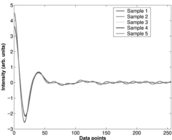
Spectral information was collected as 3000 (100 from each of 5x6=30 samples) double-sided interferograms with 1024 points. The interferograms were phase compensated and were, therefore, symmetrical about the centreburst. Conse-quently, it was possible to discard half of the data without in-curring any loss of information and the dimensionality of the feature space was reduced from 1024 to 512. The first 256 points of the mean interferograms from each coated paper are shown in Fig. 1.
FIG. 1: Plot of the mean interferograms from each coated paper obtained from the Michelson prototype instrument. The first 256 points to the right of the centreburst are shown.
simulated in Matlab with one hidden layer, whose size was systematically varied between 1 and 30 nodes. Experiments showed that further increase of the number of hidden nodes did not improve the generalization due to overfitting. For hid-den layer nodes, hyperbolic tangent transfer functions were used, whereas logistic functions were used for output layer nodes. Ten trials were attempted for each network and the MSE of prediction with the number of epochs required for convergence were recorded. The criterion for stopping train-ing was an MSE≤10−5or an increment of the validation error for a specified number of iterations.
The second data set used was from a medical applica-tion [30] and contained a total of 264 patients for which mea-surements of 21 wavelengths of the spectrum has been col-lected. For the same patients we also have measurements of HDL, LDL, and VLDL cholesterol levels, based on serum separation. The first step was to perform a principal com-ponent analysis and retain those principal comcom-ponents which account for 99.9% of the variation in the data. There is sig-nificant redundancy in the data set, since the principal com-ponent analysis has reduced the size of the input vectors from 21 to 4. The next step is to divide the data up into training, validation and test subsets. We will take 25% of the data for the validation set, 25% for the test set and 50% for the train-ing set. We pick the sets as equally spaced points throughout the original data.
A similar procedure as described above for the paper data was used, but this time the number of inputs to the net-work was fixed to 4 principal components, and an MLP was simulated in Matlab with one hidden layer, whose size was systematically varied between 1 and 30 nodes. For hidden layer nodes, hyperbolic tangent transfer functions were used, whereas linear transfer functions were used for output layer nodes. Ten trials were attempted for each network and the stopping criterion was the same as above.
We compared our proposed model to different gradient de-scent algorithms which use constant or adaptive learning rates as these methods show improved learning speed and good convergence behavior [8]. More specifically, we first applied the batch gradient descent training algorithm (TRAINGD).
1 1.25 1.5 1.75 2 −0.51
−0.5 −0.49 −0.48 −0.47 −0.46 −0.45
q
log(MSE)
FIG. 2: Mean MSE of networks with 1 to 30 nodes for 1<q<2.
Next we investigated the performance of the gradient de-scent algorithm with momentum (TRAINGDM). We also applied gradient descent with adaptive learning rate with (TRAINGDX) or without momentum (TRAINGDA). Nev-ertheless, by applying all these algorithms there is no guar-antee that the network error will monotonically decrease at each iteration and that the weight sequence will converge to a minimizer of the sum-of-squared-differences error function E. Therefore, as shown in the next section, the proposed nonextensive training schemes provide evidence that there is significantly improvement in the overall classification perfor-mance.
5. RESULTS AND DISCUSSION
To find the optimal values ofq, a series of runs were per-formed using the cholesterol data as input and changing the network’s structure. For each 0<q<5, the mean MSE of all networks (from 1 to 30 neurons) was recorded and it was found that there is an optimal area betweenq=1.2 and q=1.3. Figure 2 shows the results of the tests around that area in logarithmic scale. The minimum value of MSE is 0.3141 and is achieved for q=1.3. It is also shown that the error forqbetween 1.15 and 1.5 is lower than the error obtained withq=1.
TABLE I: Optimal topologies and MSE for MLP networks trained with spectral components of blood samples.
Training Best Best Mean (%) Improvement Method Topology MSE MSE MSE of AHTS
AHTS 4-25-3 0.220 0.349 – HTS 4-27-3 0.245 (+) 0.352 (–) 0.85%
GD 4-23-3 0.343 (+) 0.507 (+) 31.2% GDX 4-30-3 0.292 (+) 0.422 (+) 17.3% GDM 4-13-3 0.337 (+) 0.529 (+) 34.0% GDA 4-13-3 0.323 (+) 0.421 (+) 17.1%
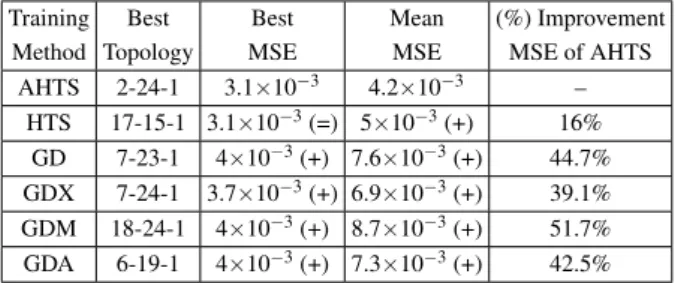
TABLE II: Optimal topologies and MSE for MLP networks trained with spectral components of coated paper data.
Training Best Best Mean (%) Improvement Method Topology MSE MSE MSE of AHTS
AHTS 2-24-1 3.1×10⁻³ 4.2×10⁻³ – HTS 17-15-1 3.1×10⁻³(=) 5×10⁻³(+) 16%
GD 7-23-1 4×10⁻³(+) 7.6×10⁻³(+) 44.7%
GDX 7-24-1 3.7×10⁻³(+) 6.9×10⁻³(+) 39.1% GDM 18-24-1 4×10⁻³(+) 8.7×10⁻³(+) 51.7%
GDA 6-19-1 4×10⁻³(+) 7.3×10⁻³(+) 42.5%
Fig. 4 shows the linear regression applied to network outputs when trained with all the schemes in test. The network struc-tures are shown in the first column of Table I. We see that the Hybrid Training Schemes give not only the lowest error but also perform better than the gradient descent algorithms tested for smaller sizes of networks.
Similar results were obtained using paper data as inputs. In this case, the error was significantly reduced compared to the network outputs with the blood samples because this is naturally an easier problem. The lowest prediction error was found to be 3.1×10⁻³and it was obtained with a 2-24-1 net-work structure. Output results can be seen in Table II.
We have evaluated the performance of the new methods and compared them with the class of the gradient descent al-gorithms. The statistical significance of the results has been analyzed using the Wilcoxon test [31]. This is a nonparamet-ric method that is considered an alternative to the paired ttest. All statements in the tables reported below refer to a signifi-cance level of 0.05. Statistically significant cases are marked with (+), while (-) shows the cases that do not satisfy the sig-nificance level.
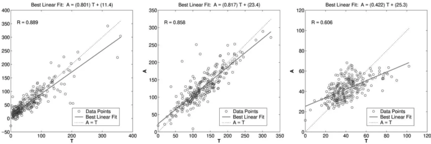
Going through the experimental results with the choles-terol data, we can conclude that the first two outputs seem to track the targets reasonably well, and the R-values are almost 0.9. The third output (VLDL levels) is not so well modeled. Improved results may be obtained with Bayesian regulariza-tion instead of early stopping for our training technique. Of course there is also the possibility that VLDL levels cannot
be accurately computed based on the given spectral compo-nents. Nevertheless, HTS and AHTS gave the best overall mean squared error and looking at the slopes of the regres-sion lines of Fig. 4 we can say that they best modelled output 1, and only TRAINGDX gave slightly better results for out-puts 2 and 3.
In any case, different data pre-processing strategies could be applied to improve network performance. Both the con-struction requirements of ANN models with correct predic-tion ability and the poor agreement between the number of spectral points and the number of spectra in small data sets require to find different strategies for the reduction of the size of the input vector. In this paper, though, we have focused on training schemes and tried to relieve the benefits of nonexten-sive statistical mechanics when applied to feedforward neural networks.
6. CONCLUSIONS
The main goal of this study was to test the performance of ANNs with nonextensive learning methods. It has been observed that they can be used as an efficient tool to esti-mate coat weights on security papers and blood cholesterol levels. Preliminary numerical results using supervised learn-ing schemes through Nonextensive Statistical Analysis, show improved performance in terms of prediction error and net-work structure compared to the best previous attempts. This is mainly because of the use of more stochastic neural schemes. In particular, the use of Adaptive Hybrid Training Scheme im-proved the network performance by as much as 34% for the classification of blood cholesterol levels and 51% for coat-ing weight estimation. To obtain these results a series of ex-periments was performed to identify the optimal values ofq. These experiments also showed that the error was reduced forq6=1 compared with that obtained forq=1. During the study, emphasis was given on the performance of smaller net-work architecture, thus reducing the computation cost. Train-ing with nonextensive statistical mechanics proved to be par-ticularly beneficial with reduced size networks. Future work will focus on exploring the use of the new method not only in spectroscopy but also in other classes of problems, possibly in combination with more efficient dimensionality reduction techniques. We also need to further investigate the perfor-mance of the new method in a restarting mode and the critical role of the temperature in the whole process.
Acknowledgments
The contributions and assistance provided by Ralph J. Houston is greatly appreciated. We also thank Arjo Wiggins Ltd for providing their paper samples. The partial financial support from the University of Patras, EPSRC and Faperj is gratefully acknowledged.
[1] A. D. Anastasiadis, G. D. Magoulas, and M. N. Vrahatis, Journal of Computational and Applied Mathematics191, 166
FIG. 3: Linear regression for outputs 1, 2 and 3 of an MLP network with 4 inputs and 27 hidden nodes trained with cholesterol data and the Hybrid Training Scheme. The regression R-values are shown on top left.
FIG. 4: Linear regression for outputs 1, 2 and 3 of MLP networks with optimal topologies (as shown in Table I) trained with cholesterol data and various learning algorithms. The slope values for each algorithm is shown on top left.
[2] A. D. Anastasiadis and G. D. Magoulas, The European Physi-cal Journal B50, 277 (2006).
[3] M. Boyukata, Y. Kocyigit, and Z. B. Guvenc, Brazilian Journal of Physics36, 730 (2006).
[4] L. Dolmatova, C. Ruckebusch, N. Dupuy, J.-P. Huvenne, and P. Legrand, Chemometrics and Intelligent Laboratory Systems 36, 125 (1997).
[5] B. Sch¨olkopf, C. Burges, and A. Smola, Advances in Ker-nel Methods-Support Vector Learning(MIT Press, Cambridge, MA, 1999).
[6] A. D. Anastasiadis, G. D. Magoulas, and M. N. Vrahatis, Pat-tern Recognition Letters26, 1926 (2005).
[7] A. D. Anastasiadis, G. D. Magoulas, and M. N. Vrahatis, Neu-rocomputing64, 253 (2005).
[8] G. D. Magoulas and M. N. Vrahatis, Neural, Parallel and Sci-entific Computations8, 147 (2000).
[9] R. Battiti, Neural Computation4, 141 (1992). [10] P. P. Van der Smagt, Neural Networks7, 1 (1994). [11] J. Nocedal, Acta Numerica1, 199 (1992). [12] G. Gyorgyi, Physics Reports342, 263 (2001).
[13] C. Tsallis and D. A. Stariolo, Physica A233, 395 (1996). [14] C. Tsallis, Statistical Physics52, 479 (1988).
[15] A. D. Anastasiadis and G. D. Magoulas, Physica A344, 372 (2004).
[16] C. Tsallis, Brazilian Journal of Physics29, 1 (1999).
[17] C. Tsallis, Physica D193, 3 (2004).
[18] H. Shibata, Physica A: Statistical Mechanics and its Applica-tions317, 391 (2003).
[19] W. H. Siekman, Chaos, Solitons and Fractals16, 119 (2003). [20] U. H. E. Hansmanna and Y. Okamotob, Brazilian Journal of
Physics29, 187 (1999).
[21] A. C. Tsallis, C. Tsallis, A. C. N. Magalhaes, and F. A. Tamarit, Complexus1, 181 (2003).
[22] S. M. D. Queir´os, L. G. Moyano, J. de Souza, and C. Tsallis, The European Physical Journal B55, 161 (2007).
[23] J. E. Straub and I. Andricioaei, Brazilian Journal of Physics29, 179 (1999).
[24] M. P. de Albuquerque, I. A. Esquef, A. R. G. Mello, and M. P. de Albuquerque, Pattern Recognition Letters25, 1059 (2004). [25] M. Gell-Mann and C. Tsallis, Nonextensive Entropy–
Interdisciplinary Applications (Oxford University Press, 2004).
[26] D. E. Rumelhart, G. E. Hinton, and R. J. Williams, inParallel Distributed Processing:Explorations in the Microstructure of Cognition 1, edited by D. E. Rumelhart and J. L. McClelland (MIT Press, 1986), pp. 318–362.
[27] C. Tsallis, R. S. Mendes, and A. R. Plastino, Physica A: Statis-tical Mechanics and its Applications261, 534 (1998). [28] D. Kalamatianos, P. Wellstead, J. Edmunds, and P. Liatsis,
[29] C. Bishop,Neural Networks for Pattern Recognition (Claren-don Press, Oxford, UK, 1995).
[30] N. Purdie, E. A. Lucas, and M. B. Talley, Clinical Chemistry 38, 1645 (1992).