http://dx.doi.org/10.1590/S1982-21702014000400050
THE VISUALIZATION AND ANALYSIS OF URBAN
FACILITY POIS USING NETWORK KERNEL DENSITY
ESTIMATION CONSTRAINED BY MULTI-FACTORS
A visualização e análise de facilidades urbanas, usando o método POIS por meio da densidade de Kernel restringida
WENHAO YU TINGHUA AI
School of Resource and Environmental Sciences, Wuhan University,
Luoyu Road 129, Wuhan, China
e-mail: [email protected] ; [email protected]
ABSTRACT
Keywords: Network Kernel Density; Network Analysis; POI (Point of Interest), Spatial Statistics.
RESUMO
No ambiente urbano, os prestadores de serviços mais importantes são normalmente representados por um conjunto de pontos em aplicações GIS utilizando o modelo POI (ponto de interesse), associado a certas atividades sociais. O conhecimento sobre a intensidade e o padrão de distribuição das facilidades - POIs (Pontos de interesse) é de grande importância na análise espacial, incluindo o planeamento urbano, a escolha do local de negócios e certas recomendações sociais. A Kernel Density Estimation (KDE) é uma eficiente ferramenta de estatística espacial para facilitar os processos apontados acima, e desempenha um papel importante na avaliação da densidade espacial, porque o método KDE considera o impacto da deterioração dos serviços e permite o enriquecimento das informações de uma forma muito simples, utilizando um gráfico de dispersão, tendo como saída uma superfície de densidade. No entanto, o KDE tradicional baseia-se principalmente na distância euclidiana, ignorando o fato de que na rede viária urbana a função de serviço POI materializa-se em uma estrutura com limitações de rede, ao invés de ser num espaço contínuo euclidiano. Visando equacionar essa questão, o presente estudo propõe um método computacional do KDE em uma rede e adota um novo método de visualização, utilizando uma superfície "parede" 3D. Alguns fatores reais condicionantes também são levados em conta neste estudo, tais como a capacidade de tráfego e a mão de direção de estradas. De forma prática, o método proposto é implementado sobre dados reais POI da cidade de Shenzhen, na China, para descrever a característica de distribuição de serviços sob impactos de multifatores. Palavras-chave: Densidade Kernel de Redes; Análise de Redes; POI (Pontos de Interesse); Estatística Espacial.
1. INTRODUCTION
and management (ANTIKAINEN, 2005; LOWE, 2005; LÜSCHER and WEIBEL, 2013).
There exists a wide range of methods to analyze such point distribution density and point pattern and can be generally classified into two broad categories (BAILEY et al., 1995): (1) The method for analyzing first-order properties, which measure the variation in the mean value of the spatial point pattern across the space (intensity), (2) The method for exploring second-order properties, which examine the spatial interaction (dependence) structure of point facilities for spatial patterns. The previous includes methods such as Quadrat analysis, Voronoi-based density estimation and Kernel Density Estimation (KDE), while the latter includes other geostatistical methods, such as Ripley’s K-function, Getis’s G-statistic and Moran’s I function. Among these methods, KDE is one of the most popular methods for analyzing the underlying properties of point events not only because of its easy-to-understand and easy-to-implement, but also because of its reflection of spatial heterogeneous of geographic process and its capacity of identifying local spatial character (ELGAMMAL et al., 2002; FLAHAUT et al., 2003; SHEATHER et al., 1991; STEENBERGHEN et al., 2004, 2010).
The purpose of KDE is to generate a smooth density surface of point events over space by computing event intensity as density estimation, and further to discover the spatial heterogeneity or inconsistency of the geographic process. Essentially, such estimator is based on Tobler’s First Law of Geography which states “Everything is related to everything else, but near things are more related than distant things” (TOBLER et al., 1979). Hence in real-world scenarios, the kernel estimator is usually used for spatial analyses on continuous phenomena including traffic hazards, environmental pollution and urban facility impacts (BAILEY et al., 1995; BORRUSO et al., 2003, 2005, 2008; XIE et al., 2008).
other global measures (e.g. Getis’s G-statistic, Moran’s I) it does not reveal the location of clusters within distribution.
Aiming at network spatial phenomena, we have two techniques to analyze the event intensity at a finer scale: the local spatial-autocorrelation method (FLAHAUT et al., 2003; STEENBERGHEN et al., 2004; GETIS et al., 2008) and the network Kernel Density Estimation (BORRUSO et al., 2003, 2005, 2008; OKABE et al., 2009b). For example, Flahaut et al. (2003) treat linear stretch of a certain length as basic spatial units (BSUs) and count the number of accidents occurred in each BSUs. Then Euclidean distances are computed between BSUs, and local Moran’s I measure is used for detecting significant clusters. In this case the computation method of planar distance metric does not consider the special nature of street networks such as connectivity and restriction of travel manner. Besides, the local-autocorrelation method requires the division of space into basic statistical units of equal size, which is available in planar space, but in network space that is variable, because too short units are often generated by irregular alignment of a network.
Attempts to resolve this dilemma have resulted in the network KDE. For example, Borruso (2008) proposed a modified KDE (termed as Network Density Estimation, or NDE for short) to analyze patterns of point events distributed over a network. He considered the kernel as a density function based on the network distance. By analyzing the resultant intensity patterns, it is possible to identify potential “hotspot” clusters along networks. However his study still used 2-D grid cells and the outcome is still mapped onto a 2-D Euclidean space. Shiode (2008) pointed out that using square grid in such cases may distort the representation of the distribution on a network. Hence a network-based quadrat method is proposed for a more accurate aggregation. Recently, the KDE method based on the network-based quadrat has been extensively explored and it is still under investigation in methodological aspects as well as in concrete applications (OKABE et al., 2006a, 2006b, 2009b; XIE et al., 2008, 2013).
a new visualization strategy of facility POIs for improving the identification of the typical “linear” clusters along roadways.
The remainder of the paper is organized as follows: Section 2 presents the extension of KDE from the Euclidean space to the network space and describes the impacts of realistic constraints on network KDE. The practical implementation of the methodology is detailed in Section 3 along with introducing of a 3-D visualization strategy. In Section 4, we present a case study with a real-world street network and four sets of selected facility POIs. Finally Section 5 presents conclusions.
2. EXTENSION OF DENSITY ESTIMATION: FROM EUCLIDEAN SPACE TO NETWORK SPACE
Spatial density is the property that describes the spatial distribution in an intensive or sparse pattern in quantity. The density estimation tries to evaluate the density value to represent the local distribution intensity. Compared with simple observation of a distribution in dot maps, the event density often acts as a refined analysis to discover the deep information behind the geographical phenomenon, for example, to detect the crime or accident ‘hotspots’, examine the cluster of business activities.
2.1 Density Estimation
The analysis over a density surface is based on the technologies of spatial smoothing and spatial interpolation (JONES, 1990; BAILEY et al., 1995). Conventionally, three methods of density analysis have been widely used in geographical analysis domain: (1) Quadrat analysis; (2) Voronoi-based analysis and (3) KDE method. Quadrat analysis drapes a grid of equal-sized and homogeneous cells (i.e. quadrats) over the study area and counts the number of event points falling in each cell to describe the spatial distribution. Voronoi-based method also needs to divide the study region into sub-regions corresponding to the partitioning cells in Voronoi construction. A Voronoi diagram is the partitioning of the plane into N polygonal regions, each of which is associated with a given point. The region associated with a point is the locus of points closer to that point on some criterion than to any other given point (GOLD, 1991, 1994). By computing the Voronoi polygons of a point set, the region of influence of each event can be achieved and the reciprocal of sub-regional area can be computed as the density value of the Voronoi sub-region (YAN and WEIBEL, 2008).
geographical continuity across the boundary of sub-region is not remained as the method doesn’t take into account the distribution in the neighborhood of grid cell. The use of KDE can improve the above situations. KDE provides an estimation of the intensity in each point of the grid by means of “moving three-dimensional functions that weight events within its sphere of influence according to their distance from the point at which the intensity is being estimated” (GATRELL et al. 1996). With the weight function, the intensity in a cell is related to the distributions in neighbor cells. Although KDE still requires the use of a grid of square superimposed cells, but as long as the mesh size is small enough, a smooth estimate of a density can be obtained for minimizing the above losses of information. Figure 1 shows the effect of these three methods on the same data. It can be observed that the advantage of KDE lies in that it allows estimation of the density at any location in the study region (O’ SULLIVAN and UNWIN, 2003).
The general form of a kernel density estimator is expressed as:
2
1
( )
1
( , )
ii n
f s
k
d s c
h
h
=
=
∑
(1)where f(s) is the density measured at location s, h the search radius (bandwidth) of the KDE (only events within h are used to estimate f(s)), ci the observed event point, k( ) the weight of event ci at distance d(s, ci) to location s. The KDE usually models the so-called kernel function, k, as a function of the ratio between d(s, ci) and h, so that the “distance decay effect” can be taken into account in density estimation. In fitting with Tobler’s first law of geography, each local weighted process is estimated with events whose influence decays with distance, distances that are commonly defined as straight line or Euclidean (Figure 1(b)).
Figure 1 - Illustration of three common methods for density estimation in planar space: (a) Quadrat analysis; (b) Kernel density estimation; (c) Voronoi-based
analysis.
The evaluation of KDE requires two parameters: The bandwidth h and the kernel function k, which determines the weighting of the points. In this study, we use the Quartic kernel function (Equation 2) which is one of the most commonly used functions:
2
2
) 3
1 ( ( , ))
4
( ,
(
c)
(
d s c)
h h
d s
k
= − (2)where function k and parameters s, c, h are the same of that in Equation 1.
According to researches (BAILEY et al., 1995; BORRUSO et al., 2003, 2005, 2008; XIE et al., 2008), the kernel function has little impact on the evaluation result. Alternatively the selection of bandwidth is a more influential factor capable of affecting the statistical results by controlling the smoothness of the estimated density. The bandwidth control behaves as that the larger the bandwidth will get smoother resultant density distribution. In reality, there are two factors to decide the choice of bandwidth. One is the spatial scale and another is the degree of dispersion between events. A small bandwidth can reveal local effects in the distribution and the larger bandwidth can reflect more clearly “hot spots” at a global scale. For sparse distribution events, the larger bandwidth is recommended, as a narrower one will not provide much more information than the simple observation of event distribution in a dot-map or scatter plot.
Both Quadrat analysis and Voronoi-based analysis for density evaluation ignore the intensity changes within each cell division, leading to abrupt changes between adjacent cells. On the contrary, the method based on KDE resolves the question of abrupt changes around the neighboring cells in density evaluation. The process of progressively transmitting center intensity by KDE takes into account “distance decay effect”, which satisfies the first law of geography. Relatively to the other two methods, the KDE method has greater potential in infrastructure planning and urban analysis (O’ SULLIVAN and UNWIN, 2003).
2.2 Kernel Density Estimation on Networks
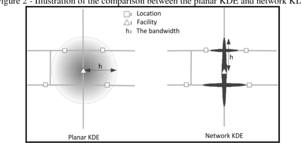
When KDE method expended from 2D Euclidean space to network space, the network KDE still preserves the principle ofnear events more related than distant events, but the distance concept changes. Moreover the event context behaves as subset of network. To illustrate the restrictiveness of network structure, Figure 2 shows an example in which the triangle stands for facility, the square the sample location and the solid line the edge of the network. It can be noted that the distance in planar KDE is measured in terms of Euclidean distance, while in network KDE it is replaced by route distance. As illustrated in Figure 2 the planar method overestimates the clustering tendency with three locations within the search bandwidth, where zero in the case of network method.
Figure 2 - Illustration of the comparison between the planar KDE and network KDE.
To analyze the distribution of facility POIs, the choice of search bandwidth h depends on three main factors, namely the data level of detail, the size of sample points and the coverage of service functionality. In addition to the first two generic factors (presented in Section 2.1), the service functionality also has a significant influence on the determination of the parameter, for example, shopping mall usually has a larger service area than retail store, and hence a larger bandwidth is fit for the distribution analysis of shopping mall’s service.
Figure 3 – The ordinary model of kernel function in a network.
2.3 Constrained Network KDE
2.3.1 Road direction
The traffic restriction, such as one-way regulation, greatly affects the service area of facilities. For example, the KFC’s delivery service chooses the optimal route from store to consumers considering traffic direction. Okabe et al. (2009a) introduces inward and outward distances for measuring the accessibility in a directed network. In terms of the two distance metrics, we also assign the network KDE into two types: inward and outward KDE. This means that the network KDE is based on the shortest paths which either lead toward the events (inward) or departure from the events (outward). Inward KDE usually is associated with facilities such as parking lots, supermarket and hospital, while outward KDE is used for other facilities such as fire stations and fast food chains. Formally Equation 3 and Equation 4 show the inward kernel function and the outward kernel function, respectively, where the distance d(s, c) is referred to as the inward distance to c, and d(c, s) is referred to as the outward distance from c. Based on the directed distances, Figure 4 shows an illustrative example of the directed kernel functions. It is observed that distances and densities on a directed network are asymmetrical, i.e. d(s, c) = d(c, s) and ( , ) ( , )
( c) (d c )
h h
d s s
k =k
does not always hold. The model functions
are useful as they allow the analysis of a real-world urban environment characterized by the presence of different functional directions.
2
2
) 3
1
( ( , ))
4
( ,
(
c)
(
d s c
)
h
h
d s
2
2
( , 3
1
( ( , ))
4
)
(
d c)
(
d c s
)
h
h
s
k
= − (4)Figure 4 - The model of kernel function in s directed network. (a) inward kernel function; (b) outward kernel function.
(a) (b)
2.3.2 Traffic capacity
2
2
) 3
1 ( ( , ))
4
( ,
(
)
'
(
t)
t t
t c d s c
h h
d s
k
= − (5)where ht is measured in terms of travel time, dt(s, c) is the travel time between location s and event c.
Figure 5 - The traffic-capacity constrained kernel function. Grey hair line represents ordinary kernel function while dark hair line represents constrained kernel function.
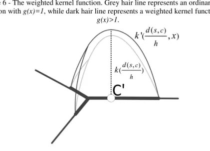
2.3.3 Event difference
In some situations, besides the facility location, the non-spatial characteristics (e.g. the prices of goods at the stores, the size of the stores, etc) of facility POIs have impacts on the service area distribution. Facilities of different types could have different attractions for people and sometimes two regions sharing a similar distribution of POIs could still have different service areas. For example, a region containing supermarket POIs is more attractive to consumers than other ones mainly containing retail stores.
Hence we formalize the weighted kernel function in the form of Equation 6, where location is weighted by combining its distance (i.e. d(s, c)) from the facility and the weight (i.e. x) of the facility. As shown inFigure 6, the larger the weight of a facility is, the more the neighbor locations are weighted for calculating the overall density.
2
2
) 3
1 ( ( , ))
4
( ,
(
)
'
c,
( )
(
d s c)
h h
d s
k
x
=g x
− (6)Figure 6 - The weighted kernel function. Grey hair line represents an ordinary kernel function with g(x)=1, while dark hair line represents a weighted kernel function with
g(x)>1.
3. IMPLEMENTATION AND VISUALIZATION
3.1 Computational Algorithm
In spatial network analysis, some researches such as Okabe et al. (2009b) and Xie et al. (2008, 2010) tend to use a linear basic spatial unit (LBSU) rather than a planar unit in network kernel density estimation. These methods are most effective when applied to a micro-scale data set, because the difference between the network distance and the Euclidean distance becomes more significant when dealing with a data set of a finer scale. However, due to the computational complexity of the shortest-path distance calculation, these methods are time-consuming. To improve the method, this section introduces a new algorithm supported by an operator of 1-D sequential expansion. The idea is inspired by the natural phenomenon that water flow extends along certain linear channels until arrives at the boundary of “sphere of influence” or at the end of route. The algorithm has the advantage that the time consuming GIS tasks (e.g. comparing for distances of potential shortest-paths) are avoided, and replaced with a linear time operation. Such operation is analogous to the dilation operator developed in mathematical morphology (HEIJMANS et al, 1990).
comes from; (3) the density-value which stores the density value calculated with the selected kernel function.
The basic algorithm is presented as follows:
(1) Divide the road network into a set of basic linear units (LBSUs) of a defined network length l. The intersection point of two LBSUs is called LBSN. Road intersections are always LBSNs.
(2) Create a LBSU-based linear reference system by establishing the network topological relationship between LBSUs, as well as between LBSUs and LBSNs.
(3) Define a search bandwidth h, measured with the number of steps of flow expansion. The bandwidth can also be measured in terms of the shortest-path network distance by using the product of h and LBSU’s length l. (4) Project facility POIs onto LBSUs, by nearest distance search. Those
LBSUs with one or more facilities assigned to them are identified as sourceLBSUs (acting as the source of stream flow). Initiate the numeric attribute steps-length of each LBSU as ∞ (infinity) and the attribute density-value as 0.
(5) Initiate set active-set. For each source LBSU, push it into active-set, and assign its attribute steps-length as 0. For each element in active-set, record its attribute flow-source the facility ID;
(6) For each element in active-set, calculate its density by repeating the expansion operation (steps a-e) until the active-set is null (see Figure 7): a. For current element q generate its next neighboring LBSUs on the basis of
the network topology, and store them in a temporary set next-LBSUs. b. Record the number of steps to next-LBSUs as their attribute
steps-length, and transform the attribute flow-source of element q to next-LBSUs.
c. Remove LBSU from next-LBSUs if its steps-length is larger than the bandwidth h.
d. Calculate the density by using the steps-length and the constrained function (f’(s)), and add it to the attribute density-value of next-LBSUs. e. Remove element q out of active-set and push next-LBSUs into
active-set.
Figure 7 - 1-D sequential expansion algorithm supported by the stream flowing simulation. (a) example of a road network with facility P (using the network-based Quadrat method); (b) distance calculation through one step expansion; (c) distance calculation through two step expansion; (d) stopping the operation when the number
of steps from the source LBSU to the boundary LBSUs is equal to or larger than the search bandwidth h (h =3 LBSUs).
They work by visiting nodes in the network, starting with the event’s start node, and then iteratively examine the closest not-yet-examined node, and add its successors to the set of nodes to be examined. Since each iteration has to compare all nodes whose shortest path to the start node is unknown, the algorithms will take a very long time to compute the network distance. Typically for the vector-based algorithms under graph theory, the time complexity is O (mn+k
log
k), where k is the number of road intersections. It can be noted that the 1-D sequential expansion algorithm is more efficient than the previous ones in terms of time complexity- that is, m+n< mn+klogk for m, n>2 and, in the practice m and n are large numbers. Furthermore for the network of Shenzhen (37932 edges and 26247 nodes, 1654(a) (b)
facility points, 160000 LBSUs) the total computation time on a modern computer was about half a minute by using our method, which yet was about two minutes by using the method in OKABE et al. (2009b).
3.2 3-D Visualization of Density Surface
To visualize the third dimension information (semantic data) in 2D space, we usually apply the vertical surface to obtain a 3D mapping effect. Borruso (2008) presented the intensity of a point pattern by means of a smoothed three-dimensional surface that represents the estimated density not only on the network but also on the region in which the network is embedded. In such visualization approach, 2-D quadrats are used to exhaustively fill out the entire planar area in the result surface, and which has no difference to the traditional visualization technique in planar KDE researches. As the context of facility POIs is treated as the network space, this approach is likely to miss out the “linear” characteristics of service distributions observed on or along a road network. Now that the intensity value of event becomes an attribute of the divided linear unit in our method, it is better to represent the density patterns by means of homogenous and comparable linear features. And, in the real world, there are many events that can be analyzed in terms of the density along the line segments forming the network. Examples include car accidents on streets, street crime sites on sidewalks, leaks in gas and oil pipelines, seabirds located along a coastline, and also facilities located alongside streets. In real-world applications, the density of the events mentioned above is usually reported as the number of points over a defined linear unit rather than over an area unit, such as accidents per mile for traffic management. Essentially the visual variables associated with drawing linear features mainly include three elements, namely, color, width and height. It can be realized by using a variable or a certain combination of two and even all three of them. In this section a new visualization strategy combining the line color and height is proposed to extract useful information from POI data more simple and effectively.
More specifically, with sequential expansion operator, the density value of POIs is firstly assigned to each LBSU as its z value (i.e. height attribute), and then based on the height of each LBSU, the original 1-D road network is extruded into a 3-D wall-like network, in which peaks (i.e. high walls) represent the presence of clusters or “hot spots” in the distribution of services. To make the visual effect more obvious and intuitive, the LBSUs are also rendered through a colour-thematic representation (Figure 8).
Figure 8 - Three-dimensional visualization of the intensity surface in (a) a small region and (b) a large region.
(a) (b)
4. CASE STUDY-THE ANALYSIS OF FACILITY POIS PATTERNS IN SHENZHEN CITY, CHINA
4.1 Experiment Data
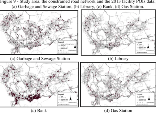
The data for this study include a real transportation network system in the Shenzhen city, China, with facility POIs for 2013 (Figure 9).
Figure 9 - Study area, the constrained road network and the 2013 facility POIs data: (a) Garbage and Sewage Station, (b) Library, (c) Bank, (d) Gas Station.
(a) Garbage and Sewage Station (b) Library
The network contains 37932 edges and 26247 nodes. The edges are classified into three levels, namely the main, the secondary and the ordinary street, depending on the average travel speed. According to the speed survey from the transformation management department, we take the speed 60 km/h, 40 km/h, and 20 km/h for three levels streets respectively, and corresponding the weight of LBSU length of the street is set as 3.0, 2.0, and 1.0 respectively. Among the network streets, some streets belong to one-way traffic. The total length of the network is approximately 8000 km. Besides we consider the category type including ‘Garbage and Sewage Station’, ‘Library’, ‘Bank’ and ‘Gas Station’, as the facility type in our experiments, and these facilities have 417, 215, 1575 and 300 data points, respectively. Due to the different natures of the data involved, these POI datasets mostly cluster in various spatial distribution patterns within the city. The proposed algorithm is implemented in a GIS environment, developed with Microsoft Visual C++ 6.0.
To reveal hot spots at a relatively finer scale, 40 m is used as the basic unit length in the experiments. The kernel function chosen is a quartic one. Through several simulations and taking into account that the length of the unit is 40 m and that the mean length of the road segments is yet 210 m, these four POI datasets are then tested at fixed search bandwidths of 300 m, 400 m, 300 m and 300 m, respectively. This setting enables the density result to retain enough details, as well as to reflect the overall trend of spatial distribution of services. Actually in other related applications, a 300 m bandwidth was also used to analyze local effects in an urban environment (THURSTAIN- GOODWIN and UNWIN, 2000; BORRUSO, 2008). Also note that the bandwidth for Library data is larger than the others, and this is because the Library POIs are distributed more sparsely. Our simulation experiments of Library showed that other narrower bandwidths such as 300 m produce a density surface with too many individual “peaks and valleys”. As Okabe et al. (2009b) presented, a larger bandwidth is fit for the visualization of a more general trend over the study region, especially for the observation of dispersed POIs data.
4.2 Results
Figure 10shows the resultant intensity distributions, which are visualized by using the method presented in Section 3.2. In these cases, each linear basic unit is extruded into a “wall” character using an extrusion value, which is achieved from the unit’s density estimation. “Peaks” consisted of high “walls” highlight the hotspots of similar functions, while “valleys” indicate the absence of services.
As one of the categories of municipal facility, Garbage and Sewage Station is closely related with city’s daily life. The facilities distributed uniformly in the city can provide service to the urban population living in different regions, and thereby can help clean up garbage and recycling, and ensure clean urban environment.
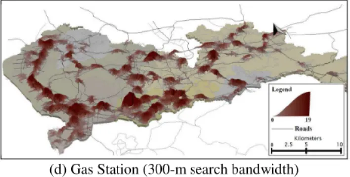
Figure 10 - Three-dimensional visualization of the distributions of services by using the proposed network KDE (40-m LBSU length, Quartic kernel), with ESRI ArcScene: (a) Garbage and Sewage Station (300-m search bandwidth), (b) Library
(400-m search bandwidth), (c) Bank (300-m search bandwidth), (d) Gas Station (300-m search bandwidth).
(a) Garbage and Sewage Station (300-m search bandwidth)
(b) Library (400-m search bandwidth)
(d) Gas Station (300-m search bandwidth)
Except for the sanitation facilities, urban managers also need to balance the requirements of the entire urban space when determining the location of Library. Figure 10(b) shows the intensity distribution of Library service, where “walls” mainly appear in the areas of Shenzhen of the Northeast, South, and West. Although the original “walls” have been stretched, the distribution of density symbols still remains low without “hot spots” appeared. So we come to the conclusion that the distribution pattern of Library in Shenzhen belongs to a type of dispersed distribution. Since Library usually has a wide coverage of service, this type of dispersed distribution meets the cultural needs of the majority of residents, and is benefit for avoiding the excessive waste of urban resources. Actually the visualization of POIs density can be a useful instrument to identify the best locations for installing new public facilities, such as Garbage and Sewage Station, Library and Hospital. In particular, urban planners would appreciate such information extracted from precise detection of “hot spots” or “absences of services”. Once “absences of services” are identified, urban planner can examine what factors around the “absences of services” contribute to the patterns and can develop effective strategies for improving the quality of life on the whole urban space.
developed (i.e. three South-North axis in the west, middle and east parts of Shenzhen). In fact, according to the Shenzhen Comprehensive Plan (2010-2020), the government planners hope that by 2020, the important service functions are undertaken in other several centers instead of just in the traditional special economic zone (south part of Shenzhen). Given present trends, the urban development and its functions evolve as its original planning.
Generally central functions such as financial and entertainment functions present a region-intensive distribution. It must be however noticed that the alignment of Gas Station service is distributed along the main roads as observed in the data intensity distribution (Figure 10(d)). We can particularly notice an increasing density and its elongation along the main roads and their parallel streets, showing a typical transportation structure of concentric rings of the Beltway. Comparing with the facilities of other types, Gas Station relies more on the local traffic conditions and hence its distribution of service is presented to be closer to the spatial patterns of city road network. In addition “peaks” in Figure 10(d) tend to appear in the outskirts of the central region and the CBD highlights a crater-like shape in the distribution. In reality, central constraints including high rents, competition of land use and traffic congestion limit Gas Station locating in the CBD of the urban area. Given that the roads, which are at the boundary of the central region, mainly take on the transportation functions to integrate the CBD with the outside, hence most of refueling services are provided along the boundary of the central region rather than inside it. In the retail sector, it is crucial to perform a solid analysis of the spatial dispersion of venders (i.e. retail facilities) because this spatial dispersion may be helpful in determining sites for new commercial establishments. For this reason, further decision making for Gas Station site location selection can be aided by combining the analysis of the intensity distribution of the venders who provide the service in the specific market.
4.3 Comparison of Ordinary Network KDE and Constrained Network KDE Figure 11 shows a small portion of the study area, i.e. Shenzhen, where one-way traffic is indicated with arrow symbols, and three levels streets is treated the same way as shown in Figure 9. Besides, we consider the weights of the Hotel points with their star rating. That is, one-star, two-star and three-star hotels are assigned weights of 1, 2 and 3 respectively in the estimating of density.
Figure 11 - The characteristics of the Hotel points (a simple Hotel’s 1-3 star rating) and of the network (road direction and road grade) in a southern part of Shenzhen,
China.
Figure 12 - The comparison of the estimated density with (a) an ordinary estimator and (b) a constrained estimator. Squares highlight absences of services where the road direction is not inconsistent with the driving direction to Hotel. Blue circles indicate where the density values are increased because of high star Hotels and high
grade road. Red circle indicates where the density pattern is not changed.
(a) Result by traditional estimator
In general, both KDE can present the density pattern of Hotels along street networks. Figure 12b demonstrates clearly how the density values along the network become sensitive to geographical constraints. Several observations can be made from a more detailed comparison. First, the ordinary KDE ideally calculates the densities on the both sides of Hotels. On the contrary, our constrained KDE ensures the densities being kept only on the reachable side of Hotels. That is, when the network quadrat obtained density value, the driving direction from its location to the Hotel is also allowed by the road direction. If such accessibility constraint is not met, the density value would be cut out (highlighted by the squares in Figure 12b, where portions correspond to density values were cut out). Our algorithm considered human behavior feature (driving from current location to hotel) in the real world and hence provided a better solution.
Second, the advantageous of accessibility was better reflected in our approach than in ordinary KDE. That is, out algorithm retains the trend that the density value on a high grade road becomes higher as driver needs less time to reach its target locations (highlighted by the the blue circles in Figure 12b). This characteristic was not respected by ordinary KDE in the corresponding segments.
The third observation is that our constrained KDE weights density values based on Hotel’s star rating, which is an important indicator of Hotel’s attractiveness. Such setting in our algorithm can ensure density values standing out in the gathering areas for high star-rated hotels (see also blue circle in the northwest of Figure 12b). Also note that, the red circle in Figure 12b highlights a region where points and local network are not constrained by any other factors, and thus such “hot spot” resembles the result by ordinary KDE. Our method takes into account geographical features beyond individual objects, so it can deal with realistic datasets better than ordinary KDE.
5. CONCLUSIONS
By using facility POIs dataset, this study presented a method to study the urban characteristics of facility context distribution and discover its behaviors at different functions (municipal services, cultural services and financial services) in a city. The present research makes four main contributions:
- Refining the search functions of traditional Kernel Density Estimation for analyzing regularity or clustering in the distribution of events, using network distances rather than Euclidean ones;
- Taking into account practical and real factors (i.e. traffic capacity, road direction, and facility difference) which are useful and desirable for real-world scenarios;
- Developing a simple and efficient algorithm based on 1-D sequential expansion to compute network distance in density estimation;
We evaluate this approach with Shenzhen road network and the related POI datasets of 2013 statistics. According to the extensive studies, the proposed method allows the visualization of the functional urban environment by means of a density surface. The discovered functional patterns can help people easily understand a complex metropolitan area, benefiting a variety of applications, such as urban planning, location choose for a business, attractive advertisements casting and social recommendations. In the future, we will further study the evolving of a city by comparing the distributions of services in different years. Besides, because traffic congestions change over time, it would be interesting to discover spatio-temporal distribution patterns.
ACKNOWLEGEMENTS
This research is supported by the National High-Tech Research and Development Plan of China under Grant No. 2012AA12A404 and 2012BAJ22B02-01. Special thanks go to Editor and anonymous reviewers for their constructive comments that substantially improve quality of the paper.
BIBILIOGRAPHICAL REFERENCES
ANTIKAINEN, J. The concept of functional urban area. Findings of the Espon project, 1, (1), p.447-452, 2005.
BAILEY, T.C.; GATRELL, A.C. Interactive Spatial Data Analysis, Longman, Harlow, 1995.
BORRUSO, G. Network density and the delimitation of urban areas. Transactions in GIS, 7, (2), p.177-191, 2003.
BORRUSO, G. Network density estimation: analysis of point patterns over a network. In: Computational Science and Its Applications–ICCSA 2005, Proceedings, p. 126-132, 2005.
BORRUSO, G. Network density estimation: a GIS approach for analysing point patterns in a network space. Transactions in GIS, 12, (3), p. 377-402, 2008. ELGAMMAL, A.; DURAISWAMI, R.; HARWOOD, D.; DAVIS, L. S.
Background and foreground modeling using nonparametric kernel density estimation for visual surveillance. Proceedings of the IEEE, 90, (7), p.1151-1163, 2002.
FLAHAUT, B.; MOUCHART, M.; MARTIN, E. S.; THOMAS, I. The local spatial autocorrelation and the kernel method for identifying black zones: a comparative approach. Accident Analysis & Prevention, 35, (6), p.991-1004, 2003.
GOLD, C. M. Problems with handling spatial data―the Voronoi approach. CISM journal, 45, (1), p.65-80, 1991.
GATRELL, A. C.; BAILEY, T. C.; DIGGLE, P. J.; ROWLINGSON, B. S. Spatial point pattern analysis and its application in geographical epidemiology. Transactions of the Institute of British geographers, 21, p.256-274, 1996. GETIS, A. A history of the concept of spatial autocorrelation: a geographer's
perspective. Geographical Analysis, 40, (3), p.297-309, 2008.
HEIJMANS, H. J.; RONSE, C. The algebraic basis of mathematical morphology I. Dilations and erosions. Computer Vision, Graphics, and Image Processing, 50, (3), p.245-295, 1990.
HAGGETT, P. Geography: A Global Synthesis. Pearson Education, Harlow, 2000. JONES, M. C. Variable kernel density estimates and variable kernel density
estimates. Australian Journal of Statistics, 32, (3), p.361-371, 1990.
LOWE, M. The regional shopping centre in the inner city: a study of retail-led urban regeneration. Urban Studies, 42, (3), p.449-470, 2005.
LU, Y.; CHEN, X. On the false alarm of planar K-function when analyzing urban crime distributed along streets. Social science research, 36, (2), p.611-632, 2007.
LÜSCHER, P.; WEIBEL, R. Exploiting empirical knowledge for automatic delineation of city centres from large-scale topographic databases. Computers, Environment and Urban Systems, 37, p.18-34, 2013.
MILLER, H. J. Market area delineation within networks using geographic information systems. Geographical Systems, 1, (2), p.157–173, 1994.
O'SULLIVAN, D.; UNWIN, D. J. Geographic information analysis. John Wiley and Sons, 2003.
OKABE, A.; OKUNUKI, K. I.; SHIODE, S. SANET: a toolbox for spatial analysis on a network. Geographical Analysis, 38, (1), p.57-66, 2006a.
OKABE, A.; OKUNUKI, K. I.; SHIODE, S. The SANET toolbox: new methods for network spatial analysis. Transactions in GIS, 10, (4), p.535-550, 2006b. OKABE, A.; BOOTS, B.; SUGIHARA, K.; CHIU, S. N. Spatial tessellations:
concepts and applications of Voronoi diagrams. vol 501, Wiley.com, 2009a. OKABE, A.; SATOH, T.; SUGIHARA, K. A kernel density estimation method for
networks, its computational method and a GIS‐based tool. International Journal of Geographical Information Science, 23, (1), p.7-32, 2009b.
SHEATHER, S. J.; JONES, M. C. A reliable data-based bandwidth selection method for kernel density estimation. Journal of the Royal Statistical Society, Series B, 53, (3), p.683-690, 1991.
STEENBERGHEN, T.; DUFAYS, T.; THOMAS, I.; FLAHAUT, B. Intra-urban location and clustering of road accidents using GIS: a Belgian example. International Journal of Geographical Information Science, 18, (2), p.169-181, 2004.
STEENBERGHEN, T.; AERTS, K.; THOMAS, I. Spatial clustering of events on a network. Journal of Transport Geography, 18, (3), p.411-418, 2010.
TOBLER, W. R. Smooth pycnophylactic interpolation for geographical regions. Journal of the American Statistical Association, 74, (367), p.519-530, 1979. THURSTAIN‐GOODWIN, M.; UNWIN, D. Defining and delineating the central
areas of towns for statistical monitoring using continuous surface representations. Transactions in GIS, 4, (4), p.305-317, 2000.
URBAN PLANNING LAND AND RESOURCES COMMISSION OF SHENZHEN MUNICIPALITY. Shenzhen Comprehensive Plan (2010-2020). Accessed 25/02/14. http://www.szpl.gov.cn/xxgk/csgh/csztgh/201009/ t20100929_60694.htm.
XIE, Z.; YAN, J. Kernel density estimation of traffic accidents in a network space. Computers, Environment and Urban Systems, 32, (5), p.396-406, 2008. XIE, Z.; YAN, J. Detecting traffic accident clusters with network kernel density
estimation and local spatial statistics: an integrated approach. Journal of Transport Geography, 31, p.64-71, 2013.
YAMADA, I.; THILL, J. C. Comparison of planar and network K-functions in traffic accident analysis. Journal of Transport Geography, 12, (2), p.149-158, 2004.
YAMADA, I.; THILL, J. C. Local indicators of network constrained clusters in spatial point patterns.Geographical Analysis, 39, (3), p.268-292, 2007.
YAN, H.; WEIBEL, R. An algorithm for point cluster generalization based on the Voronoi diagram. Computers & Geosciences, 34, (8), p.939-954, 2008.