ABSTRACT: This paper concerns a numerical optimization method for designing airfoils based on adjoint method. The goal of present work is to reduce the compressibility drag or pitching moment of transonic airfoils without compromising on the lift coeficient. A new cost function based on this requirement is deined and the corresponding adjoint equations are discussed in details. At the end, by demonstrating some numerical results, we show that this technique is capable of converging to the optimum design point corresponding to the initial geometry of the airfoil.
KEYWORDS: Optimization, Pitching moment, Transonic airfoils, Adjoint equations, Euler equations.
Optimization of Airfoils for Minimum
Pitching Moment and Compressibility
Drag Coeficients
Hamid Farrokhfal1, Ahmad Reza Pishevar2
INTRODUCTION
Improvement of aerodynamic performance of helicopter blade designs has been one of the most important research areas in rotorcraft aerodynamics. Low-pitching-moment airfoils found application primarily as helicopter rotor blades, but some attention has been given to the advantages of low pitching-moment sections for a “span-loader” vehicle. For such applications, a symmetric airfoil could conceivably be employed, but cambered airfoils can ofer signiicant advantages (Barger, 1975). herefore, designing cambered airfoils with low pitching-moment is attractive in helicopter blade design to achieve small control forces in rotor controls, and this task can be conducted via optimizing procedures.
Also, shock waves in transonic low not only increase the wave drag but also cause unfavourable lutter or bufet to ixed wings. Helicopter rotor blades in forward light are also frequently exposed to strong unsteady shock waves at the blade tip region. hese shock waves increase the required torque, and become a source of undesirable noise and vibration. hus, elimination or possible reduction of the strength of these shock waves would be desirable for the enhancement of the performance of helicopters and airplanes.
In order to improve airfoil performance under diferent light conditions and to make the performance insensitive to of-design condition at the same time, Yu et al. (2010) have developed a multi-objective optimization approach considering robust design and applied it to airfoil tailoring. hey used non-uniform rational B-spline (NURBS) representation, control points and related weights around airfoil as design variables. hey could
1.Malek-Ashtar University of Technology – Isfahan – Iran 2.Isfahan University of Technology – Isfahan – Iran.
Author for correspondence: H. Farrokhfal | Department of Mechanical & Aerospace Engineering | Malek-Ashtar University of Technology – 83145-115 | Shahinshahr – Isfahan – Iran | Email: [email protected]
obtain a set of non-dominated airfoil solutions with robustness, by adopting multi-objective genetic algorithm that is based on non-dominated sorting. hey showed that the multi-objective robust design method makes the airfoil performance robust under diferent of-design conditions.
In the gradient-based optimization design, the gradients of cost/constraint functionals with respect to design variables are important information in the design processes (Xie, 2002). A traditional approach to calculate gradients is the finite difference method which involves finite differencing performance functionals computed from the solutions to the governing equations with perturbed parameter values. he Finite diference method (FDM) with complex variables was explored by Anderson et al. (2001) to improve its accuracy. Even though it is very easy to implement FDM in program coding, its prohibitive computational costs (many times solving governing equations) motivate other time-eicient methods to calculate reduced gradients.
A way of performing an efficient aerodynamic shape optimization is to regard the design problem as a control problem in which the control is the shape of the boundary. his approach to optimal aerodynamic design was introduced by Jameson (1988, 1990) who examined the design problem for compressible low with shock waves, and devised adjoint equations to determine the gradient for both potential low and also lows governed by the Euler equations (Jameson, 1995; Reuther and Jameson, 1994).
Also, particular interest has been given to adjoint methods (Reuther et al., 2001) in which the gradient, regarding an arbitrarily large number of parameters, can be calculated with roughly the same computational cost as two low solutions. Once the gradient has been calculated, a descent method can be used to determine a shape change which will make an improvement in the design.
Based on the idea of adjoint method, an optimum aerodynamic design technique is presented by Ying et al. (2011), which can be applied to the optimum problems with a large number of design variables. he key of this method lies in that the optimization process is regarded as an unsteady evolution, i.e., the optimization is executed, simultaneously with solving the unsteady low governing equations and adjoint equations. During the unsteady evolution, the airfoil surface is moving with time, and the dynamic grid technique is introduced in the grid generation to improve the computational eiciency (Ying et al., 2011).
Nadarajah and Tatossian (2008) also have presented an adjoint method for the multi-objective aerodynamic shape optimization of unsteady viscous lows. heir method is beneicial when both the pitching angle and free stream Mach number are sinusoidally varied. hey showed that the multi-objective cost function was able to preserve both the lit and pitching moment while simultaneously decreasing the overall drag (Nadarajah and Tatossian, 2008).
Gradient-based techniques are eicient direct aerodynamic shape optimization (ASO) methods for both incompressible and compressible lows, and many of them use continuous adjoint methods.
More recently, the introduction of surrogate-based optimization (SBO) methods to ASO have been successful in reducing the total computational cost. The overall objective of using SBO methods is to reduce the number of evaluations of the high-fidelity models, and thereby making the optimization process more efficient. Leifsson and Koziel (2010) introduced a computational design methodology which exploits surrogates constructed using low-fidelity flow analysis models and shape-preserving response prediction technique and demonstrated that their approach allows a rapid design improvement of airfoils at a very low computational cost corresponding to a few evaluations of the high-idelity model (Leifsson and Koziel, 2010).
hen they replaced the direct optimization of an accurate, high idelity airfoil model by an iterative re-optimization of a corrected low-idelity model (Leifsson et al., 2011). heir low-fidelity model is based on the same governing fluid flow equations as the high-fidelity one, but uses coarser discretization and related convergence criteria. With these techniques, they succeeded to improve the overall robustness of the optimization algorithm.
ASO problems in compressible viscous flow were also performed using simultaneous pseudo-time stepping (Hazra
et al., 2005). Hazra et al. (2005) could optimize airfoil surface by use of a preconditioner for convergence acceleration which stems from the reduced sequential quadratic programming (SQP) methods.
used to discrete governing equations. his scheme employs a cell centered discretization technique. A multistage time-stepping algorithm is used to advance the solution in time. A key feature in this scheme is applying the dissipative terms at the end of each time step for solving the flow and adjoint equations. he magnitude of the dissipative terms is adapted to the local properties of the low by means of a Jameson sensor (Nadarajah and Jameson, 2001), based on the local pressure gradient. Acceleration techniques are applied to obtain faster steady-state convergence. hese methods include local time stepping, variable coeicient implicit residual smoothing, and multi grid technique.
GOVERNING EQUATIONS
Let (u,v) denote the velocity components in the Cartesian coordinate system (x,y). Compressible Euler equations can be formulated as:
(1)
Where:
(2)
Deining the lux vecto r as , where are the unit vectors in the (x, y) coordinate system, Eq. 1 can be written as:
(3)
Equation 3 can be solved by the inite-volume method described in the proceeding section.
NUMERICAL METHOD
In order to apply the inite-volume method, Eq. 3 is written in the integral form as:
(4)
he computational domain is meshed by a multi-block structured quadrilateral grid. Applying Eq. 4 to a typical (i,j) cell, for a cell center algorithm we obtain a system of ordinary diferential equations as:
(5)
Where is the cell area and represents the net convectional luxes out of each cell.
he convective luxes can be determined by a second order central scheme. However, the resultant scheme is not dissipative, and therefore, undamped oscillations at odd and even mesh points can be developed during the computation. To suppress the tendency for odd-even decoupling and to prevent the appearance of oscillations in regions containing severe pressure gradients near shock waves and stagnation points, the inite-volume scheme is modiied by the addition of artiicial dissipative terms as below:
(6)
Where denotes the dissipative luxes. Jameson has established that an efective form of dissipative terms for lows with discontinuities is a blend of second and fourth diferences with coeicients which depend on the local pressure gradient (Jameson et al., 1981). Equation 6 can be integrated in time by a multistage Runge-Kutta scheme.
BOUNDARY CONDITIONS
than a single block for a two-dimensional body, the attachment boundary condition should be used for the neighboring cells at the block interfaces. his can be done by considering a layer of ghost cells around each block. he boundary condition at the airfoil surface is the tangency condition of low, that is:
(7)
Where is the velocity vector and is the unit vector normal to the airfoil surface.
Far-ield boundary condition is also applied at the outer surface of the domain. he treatment of the far-ield boundary condition is based on the concept of Riemann invariants for a one-dimensional low normal to the boundary (Jameson and Baker, 1983).
DERIVATION OF THE INVISCID
ADJOINT TERMS
The main objective of the present study is to achieve a modiied airfoil which minimizes the inviscid compressibility drag without compromising the pitching moment under the constraint of maintaining the desired lit level. For this purpose, using the Lagrange multiplier, the cost function is deined as:
(8)
Here and are the weight coefficients by which the airfoil shape can be modified for a particular application. When is chosen to be much larger than , a reduction in the drag coefficient is the main priority of the designer while using a larger leads to an airfoil with smaller pitching moment coefficient. In this equation indicates the desired value of . The variation of cost function in relation to the angle of attack and other parameters can be written as:
(9)
Where |(.) denotes the partial derivative at the frozen quantity (.) and G denotes the low or design variables. From Eq. 9, the Lagrange multiplier σ can be obtained as:
(10)
Substituting into Eq. 9 yields:
(11)
Where:
he airfoil lit, drag and pitching moment coeicients can also be written as:
(12)
Where is the reference point for computing the pitching moment and and are the components of unit vector normal to the airfoil surface.
Taking variation from the steady state low equations in the computational domain leads to:
(13)
Where:
(14)
Finally, this equation can be integrated by parts to give:
(15)
hus, the variation in the cost function can be written as:
(16)
and n1=0 on boundary B.
Eliminating the term which contains δw from the above integrals, the adjoint equation can be obtained as:
(17)
Because n1=0 on airfoil surface, the only remaining component of Fk is:
(18)
Where from the tangent boundary condition of low on the airfoil surface, the variation of F2 becomes:
(19)
If the coordinate transformation is such that δS is negligible in the far ield, then the boundary condition of adjoint Eq. 17 can be obtained as:
(20)
Where: . Finally we have:
(21)
And the gradients can then be deined with respect to the design variables xi as:
NUMERICAL METHOD FOR ADJOINT
EQUATIONS
he semi discretized adjoint equations of Eq. 17 is obtained using the same approach used for the low equations:
(23)
Introducing the artiicial dissipation term to the Eq. 23 is crucially important to avoid discontinuities and to keep vector variable ψ diferentiable. he ive stage modiied Runge-Kutta time stepping scheme is used to march the adjoint equations to the steady-state limit. Further details of the procedure of obtaining Eqs. 17 to 23 can be found in Jameson (1990, 1995).
OPTIMIZATION ALGORITHM
A simple optimization algorithm can be established by using a line search method. These methods require an algorithm to choose a direction p and search along this direction from the current design variables to obtain a new set of variables for the cost function value. Once the direction is chosen, then a step length λ is multiplied to the search direction to advance the optimization to the next iteration. A simple optimization algorithm can be defined by setting the search direction l=-G, to the negative of the gradient at every iteration:
(24)
With a line search method, the step size λ is chosen so that the maximum reduction of the objective function I(X) is attained. he search procedure used in this work is a descent method, in which small steps are taken in a direction deined by the smoothed gradient. X represents the design variable, and G= the gradient. Instead of making the step:
(25)
We replace the gradient by a smoothed value to guarantee the generation of a sequence of smooth shapes. When smoothing is performed in the x direction, the smoothed gradient may be calculated from a discrete approximation to:
(26)
where ε is the smoothing parameter.
Finding the new position of the boundary mesh points is also necessary, in order to estimate the variation of internal nodes accordingly. Jameson (1986, 1990) introduced a grid perturbation method that modiies the current location of the grid points based on perturbations at the geometry surface. his allows the variation of the grid point location in the equation for gradient evaluation, to be substituted with the variation of the surface points. he Optimization procedure can inally be summarized as follows:
a. Solve the low equations for ρ, u1, u2, p and e.
b. Solve the adjoint equations for ψ subject to appropriate boundary conditions.
c. Evaluate the gradients and calculate the corresponding smoothed gradient ;
d. Update the shape based on the direction of steepest descent ;
e. Solve the adjoint equations again for determining the gradients and consequently for updating angle of attack by using the equation:
or:
(27)
where δXs is the perturbed coordinates of nodes on the airfoil surface, obtained in step (d); and
RESULTS
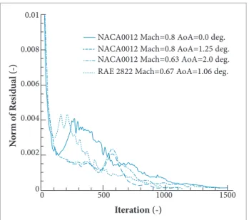
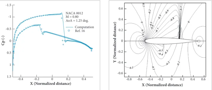
In this section, we irst validate our low solver code by simulating several benchmark problems for the transonic inviscid low over airfoils. For this purpose, transonic low over NACA 0012 and RAE 2822 airfoils are considered. he validation is performed by comparing the obtained results to the previously published results by Pulliam et al. (1983) and Cook et al. (1979). In all cases, the far boundaries are located 5 chords away from the center of the airfoil. he NACA airfoil is set to three low conditions: I) M∞=0.63, α=2.0°; II)
M∞=0.8, α=0.0°; III) M∞=0.8, α=1.25° and the free stream Mach number and the angle of attack for the RAE airfoil is IV)M∞=0.67, α=1.06°.
he Courant number number was taken as 4.0 and ive orders of magnitude reduction in the density residual is considered as the convergence criteria. In all cases, the convergence criterion is met in less than 1,500 time steps, as shown in Fig. 1.
The computational grid consists of 128 × 33 nodes stretched near the leading and trailing edges. he grid is also clustered towards the airfoil surface. Computations were performed on a personal computer with a dual core CPU for which the computational time for the aforementioned cases is less than 2 minutes.
he pressure coeicients Cp on the upper and lower surface of the airfoils are shown in Figs. 2 to 5 and compared with the other computational results. In these Figures, X has been normalized and denotes the distance from the airfoil centre. he agreement between the Euler calculation and the other reference data is obvious. Figures 6 to 8 display the pressure contour plots for case III and IV. he smoothness of rapid expansion near the nose region on the upper surface is notable. he results prove that the region near stagnation point is calculated without any excessive numerical diiculty.
his problem is very important for the shape optimization procedure and can deteriorate the smoothness of surface. In all cases, the shock location is also computed accurately with a resolution of 2 to 3 grid points. Case III is a more diicult one, where a strong shock forms on the upper surface and a weak shock on the lower one. he grid is clustered near the shock position on the upper-lower surfaces of the airfoil for this case.
he performance of the optimization algorithm for the cost function is examined and the efects of weight coeicients k1
and k2 are explored. As our irst test case, we set k1=1.0 and
NACA0012 Mach=0.8 AoA=0.0 deg.
RAE 2822 Mach=0.67 AoA=1.06 deg. 0.01
0.008
0.006
0.004
0.002
0
0 500 1000 1500
Iteration (-)
N
o
rm o
f R
es
id
u
al (-)
NACA0012 Mach=0.63 AoA=2.0 deg. NACA0012 Mach=0.8 AoA=1.25 deg.
Figure 1. Convergence History of solutions.
0
0 -0.2
-0.4 0.2 0.4
Ref. 16 Computation NACA 0012 M = 0.63 AoA = 2.0 deg.
-0.5
0.5 -1
1 -1.5
1.5
C
p (-)
X (Normalized distance)
Figure 2. Comparison of pressure distribution for the case I.
k2=0.0, therefore, reducing the problem to a pressure drag minimization one. NACA 0012 airfoil is considered to be the initial geometry and the low variables are set to M∞=0.75 and angle of attack α=3.0°.
for which the drag coefficient is minimum while the lift coefficient is maintained at the same value of Cl=0.656. An implicit smoothing technique is also used to smooth out the gradients before modifying the location of each point on the airfoil surface.
The convergence is quickly attained by this optimizing technique and only after four design cycles the drag coefficient is reduced to one third of its initial value under the fixed lift coefficient constraint Cl = 0.656 . Comparisons of the pressure distribution for the new geometry in this figure and for the initial NACA 0012 indicate that the upper surface
nodes are modified in a way that the local Mach number and the strength of the shock are attenuated on this surface. This, in turn, may lead to a lower wave drag but decreases the lift coefficient as well. As a result, the fall in the lift coefficient is compensated by modifying the shape of the trailing edge, as shown in Fig. 9 to recover the pressure difference near this region.
Figure 9 illustrates that the final design shaped is achieved after 50 designed cycles. The upper surface shock disappeared from the pressure distribution results and the drag coefficient is reduced to Cd=0.0448 , i.e., one eighth of its initial value.
0
Ref. 16 Computation NACA 0012 M = 0.80 AoA = 1.25 deg.
-0.5 0.5 -1 1 -1.5 1.5 C p (-)
X (Normalized distance)
0 -0.2
-0.4 0.2 0.4
Figure 4. Comparison of pressure distribution for the case III.
0.6 0.4 0.2 0 -0.2 -0.4 -0.6 Y (N o rm aliz ed di sta n ce)
X (Normalized distance)
-0.4 -0.6
-0.8 -0.2 0 0.2 0.4 0.6
Figure 6. Pressure contour plots for the case III.
0
Ref. 17 Computation RAE 2822 M = 0.75 AoA = 1.0 deg.
-0.5 0.5 -1 1 -1.5 1.5 C p (-)
X (Normalized distance)
0 -0.2
-0.4 0.2 0.4
Figure 5. Comparison of pressure distribution for the case IV.
0
Ref. 16 Computation NACA 0012 M = 0.80 AoA = 0.0 deg.
-0.5 0.5 -1 1 -1.5 1.5 C p (-)
X (Normalized distance)
0 -0.2
-0.4 0.2 0.4
0 -0.5
0.5 -1
1 -1.5
C
p (-)
Figure 8. Inviscid drag minimization of NACA 0012, N=0.75,
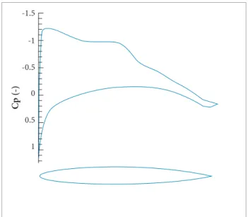
Cl=0.656, Initial Solution, Cd=0.0345, Cm=-0.0335, α=3.00º.
Convergence History Drag Coeficient
0.005 0.01 0.015 0.02 0.025 0.03 0.035 0.004
C
d (-)
Cycle (-)
5 10 15 20 25 30 35 40 45 50
Figure 10. Convergence history of drag minimization of
NACA 0012 airfoil. 0.6
0.8 1
0.4
0.2
0
-0.2
-0.4
-0.6
Y (N
o
rm
aliz
ed di
sta
n
ce)
X (Normalized distance)
-0.4 -0.6 -0.8
-1 -0.2 0 0.2 0.4 0.6
Figure 7. Pressure contour plots for the case IV.
0 -0.5
0.5 -1
1 -1.5
C
p (-)
Figure 9. Inviscid drag minimization of NACA 0012, M=0.75,
After 50 design iterations, Cl=0.656, Cd=0.0448, α=1.45º.
As can be seen in this Figure, the optimal shape is no longer symmetric, and a cusped shape is developed at the trailing edge.
he convergence history of the gradient norm and the drag coeicient are shown in Figs. 10 to 11. hese Figures indicate that the convergence rate of the procedure is fast and that the optimization is accomplished mostly in the early cycles.
It is also required to show that the inal result depends on the initial geometry. In order to do so, we repeat the computations
for a ive digit NACA 23012 airfoil as the initial geometry and change the angle of attack to reach the same lit coeicient as in the previous example.
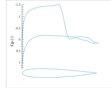
conditions. We also notice that in this drag minimization problem, the pitching moment of the optimal shape is unfavorably increased from Cm=-0.0558 to Cm=0.154.
As our second example, the other extreme case of k1=0.0 and k2=1.0 is considered, i.e., the pitching moment coeicient is minimized under the constant lit constraint and without restricting the drag coeicient. he initial geometry and low conditions are as in the previous example. As shown in Fig. 14, there is a 94% reduction in the pitching moment for the
optimal shape, while the lit coeicient remains almost constant. he drag coeicient has also shown a 23% increase.
To minimize the drag coeicient under constant lit and pitching moment coeicient, the weight constants are set to k1=0.50 and k2=0.50.
Figure 15 indicates the obtained results for the same initial airfoil geometry and the low conditions. he obtained results revealed that the drag coeicient is reduced by 76% while the lit and pitching moment coeicients are remained constant. his is the optimal shape for an airfoil that can reduce the compressible
0 -0.5
0.5 -1
1 -1.5
C
p (-)
Figure 12. Inviscid drag minimization of NACA 23012
M=0.75, Cl=0.660, Initial solution, Cd=0.0433, Cm=-0.0558,
α
=1.24º.0 -0.5
0.5 -1
1 -1.5
C
p (-)
Figure 14. Pitching moment minimization of NACA 0012,
M=0.75, After 36 design iterations, Cl=0.656, Cd=0.0424, Cm=-0.0002,
α
=3.71º.0 -0.5
0.5 -1
1 -1.5
C
p (-)
Figure 13. Inviscid drag minimization of NACA 23012,
M=0.75, Final Solution, Cl=0.660 Cd=0.0436,
α
=-0.17º.Convergence History Norm of Gradient
0.1 0.15 0.2 0.25
C
d (-)
Cycle (-)
0 10 20 30 40 50
Figure 11. Decrement of gradient norm of drag
0 -0.5
0.5 -1
1 -1.5
C
p (-)
Figure 15. Optimization of NACA 0012, k
1=0.50, k
2=0.50,M=0.75, After 32 design iterations, Cl=0.656, Cd=0.0059, Cm=-0.0338,
α
=2.65º.pressure drag at a given required lit without compromising the pitching moment coeicient.
he test cases above show that the proposed cost function for the ASO is very eicient for designing airfoil with speciic requirements in subsonic and transonic lows.
CONCLUSION
An eicient methodology for ASO of airfoils in transonic or high subsonic regime was described. In this approach, the Euler equations are solved for a symmetric and asymmetric airfoil with a multi-block method. he results obtained from this approach for the pressure distribution on the airfoil surface were
validated and it was shown that the aerodynamic coeicients are estimated with a rather good accuracy. hen the prepared solver is employed to optimize the airfoils based on the adjoint method for minimum pressure drag, while maintaining the lit and pitching moment coeicients.
hen, a new cost function was introduced for the problem of reducing the pitching moment and drag coeicients under the constant lit constraint. he procedure was irst tested for the extreme case of reducing pitching moment under the constant lift constraint without restricting the drag coeicient which was led to a inal shape with higher wave drag coeicient. However, by proper selection of cost function weight coeicients, it is possible to reduce the wave drag under constant pitching moment and lit coeicients. In this case, the inal solution is an airfoil with a sharp trailing edge and a narrow leading edge.
Drag minimization of airfoils, in the case of constant lit coefficient, has led to a cusped shape of trailing edge and relatively lat upper surface in both symmetric and cambered airfoils; but the inal solution is diferent for two cases, especially for the shape of leading edge of the airfoils.
These results indicate that the optimization procedure based on the adjoint method depends on the initial shape of airfoil. In other words, this technique can converge to a local extremum and not a global one.
he main advantage of this method is that satisfactory results can be achieved by minimum computational eforts, particularly for the grid generation problem and the required central processing unit of computer (CPU) time. his feature becomes important where a low idelity accurate case such as rotor blade low solver is required for primarily design or optimization purposes. However, the proposed method ignores important phenomena such as the viscous low or shock boundary layer interactions.
REFERENCES
Anderson, W.K., Newman, J.C., Whitield, D.L. and Nielsen, E.J., 2001, “Sensitivity analysis for Navier-Stokes equations on unstructured meshes using complex variables”, AIAA Journal, Vol. 39, No. 1, pp. 56-63. doi:10.2514/2.1270.
Barger, R.L., 1975, “Procedures for the design of low-pitching-moment airfoils”, NASA TN D-7982.
Cook, P.H., Mc Donald, M.A. and Firmin, M.C.P., 1979, “Aerofoil RAE 2822 pressure distributions, and boundary layer and wake measurement”, AGARD Advisory Report No. 138.
Jameson, A., 1986, “Multigrid algorithms for compressible low calculations”, Proceedings of the 2nd European Conference on Multigrid Methods II, Lecture Notes in Mathematics, No.1228, pp. 166–201.
Jameson, A., 1988, “Aerodynamic design via control theory”, Journal of Scientiic Computing, Vol. 3, No. 3, pp. 233-260.
Jameson, A., 1995, “Optimum aerodynamic design using CFD and control theory”, AIAA Paper 95-1729-CP.
Jameson, A. and Baker, T.J., 1983, “Solution of Euler equations for complex conigurations”, AIAA, pp. 83-1929.
Jameson, A., Schmidt, W. and Turkel, E., 1981, “Numerical solution of the Euler equations by inite volume methods using Runge-Kutta time-stepping schemes”, AIAA, pp. 81-1259.
Hazra, S.B., Schulz, V., Brezillon, J. and , Gauger, N., 2005, “Aerodynamic shape optimization using simultaneous pseudo-timestepping”, Journal of Computational Physics, Vol. 204, No. 1, pp. 46-64. doi:10.1016/j.jcp.2004.10.007.
Leifsson, L., Koziel, S. and Ogurtsov, S., 2011, “Inverse design of transonic airfoils using variable-resolution modeling and pressure distribution alignment”, Procedia Computer Science, Vol. 4, pp. 1234-1243. doi:10.1016/j.procs.
2011.04.133.Leifsson, L. and Koziel, S., 2010, “Multi-idelity design optimization of transonic airfoils using shape-preserving response prediction”, Procedia Computer Science, Vol.1, No. 1, pp. 1311-1320. doi:10.1016/j.procs.2010.04.146.
Nadarajah, S. and Tatossian, C., 2008, “Multi-objective aerodynamic shape optimization for unsteady viscous lows”, Journal of Optimization and Engineering, Vol. 11, No. 1, pp. 67-106. doi: 10.1007/s11081-008-9036-4.
Nadarajah, S. and Jameson, A., 2001, “Studies of the continuous and discrete adjoint approaches to viscous automatic aerodynamic shape optimization”, AIAA 2001-2530, AIAA 15th. Computational Fluid Dynamic Conference, Anaheim, Ca, June 11-14.
Pulliam, T.H., Jespersen, D.C. and Childs, R.E., 1983, “An enhanced version of an implicit code for the Euler equations”, AIAA-83-0344. January 10-13, Reno, Nevada.
Reuther, J.J., Jameson, A., Alonso, J.J., Rimlinger, M.J. and Saunders, D., 2001, “Constrained multipoint aerodynamic shape optimization using an adjoint formulation and parallel computers”, parts 1 and 2, Journal of Aircraft, Vol. 36, No. 1, pp. 51-74.
Reuther, J. and Jameson, A., 1994, “Control based airfoil design using the Euler equations”, AIAA paper 94-4272-CP.
Xie, L., 2002, “Gradient-based optimum aerodynamic design using adjoint methods”.
Ying, G.Y., Feng, H. and Yu, S.M., 2011, “Aerodynamic airfoil design using the Euler equations based on the dynamic evolution method and the control theory”, Science China Physics, Mechanics and Astronomy, Vol. 54, No. 4, pp. 697-702. doi:10.1007/s11433-011-4287-z.