ABSTRACT: The correlation of a model with test results is a common task in engineering. Often genetic algorithms or adaptive particle swarm algorithms are used for this task. In this paper another approach is presented using two quasi-Newton algorithms of the class deined by Broyden. A study was conducted with thermal models showing the performance of this approach. Comparing the results to other studies reveals that the approach reduces the number of iterations by several orders of magnitude; typical calculation times for model correlation times are reduced from the order of weeks and months to the order of hours and days.
KEYWORDS: Thermal vacuum test, Thermal analysis, Correlation, Broyden, ESATAN, Thermica.
On Using Quasi-Newton Algorithms of the
Broyden Class for Model-to-Test Correlation
Jan Klement1INTRODUCTION
In every calculation, there are always discrepancies between the predictions of a mathematical model and their physical measurements. Refinement of the models can reduce the discrepancies, however, the exact values of many parameters are often unknown. Without perfect knowledge of the values of these parameters, a model refinement will never lead exactly to the measured results.
Determining the exact values of all parameters individually is too costly or sometimes even impossible. Testing is often only possible at the system level, and extracting parameter values from the test results is a difficult task which is done by correlating the mathematical model with the measurement data. This means that the model parameters are changed via feedback from the measurement results, so that the discrepancies between the measurements and the models are minimized.
Many methods have been developed and analyzed to perform model-to-measurement correlation (Jouffroy, 2007; De Palo et al., 2011; Momayez et al., 2009; Harvatine and De Mauro, 1994; Roscher, 2006; van Zijl, 2013; WenLong et al., 2011; Mareschi et al., 2005). Most methods are based on stochastic optimization algorithms and often require several hundred iterations to converge. In this paper, an approach is presented using Broyden’s class of methods (Broyden, 1965), which use considerably less iterations for the majority of cases.
1.Tesat-Spacecom GmbH & Co – Backnang – Germany
Author for correspondence: Jan Klement | KG, Gerberstraße 49 | D-71522 Backnang – Germany | Email: [email protected]
THE THERMAL MODEL
CORRELATION PROBLEM
The method will be presented with a typical thermal model correlation as used in the space industry, but the procedure can also be applied to many other models as used in other industries and areas.
Thermal models calculate temperatures at certain points depending on a set of parameters. Mathematically expressed, this means:
tmdl = F(p), (1)
where:
F is the mathematical model with function F:Rk→Rm (k is the number of parameters, m is the number of results);
tmdl is a vector containing the temperatures at the selected points; and p is a vector containing the parameters of the model, for example thermal conductivity, thermal capacity, thermal emissivity, and solar absorptivity.
During the tests, the temperatures are measured at the same points as described in the model tmdl. The aim of the correlation is to find the set of parameters pcorr for which the root sum square of the differences between the measured temperatures tmes and the calculated temperatures F(pcorr) is minimal.
||F(Pcorr) – tmes|| = min{||F(p) – tmes|||p ∈ P} (2) where P is the solution space for the parameter vector.
THE METHOD
In contrast to most correlation methods developed (Jouffroy, 2007; De Palo et al., 2011; Momayez et al., 2009; Harvatine and DeMauro, 1994; Roscher, 2006; van Zijl, 2013; WenLong et al., 2011; Mareschi et al., 2005), this method will not attempt to minimize the length of the vector ||F(p) – tmes||, but searches a root of the equation system:
F(pcorr) – (tmes) = 0. (3)
he advantages of this method are that a whole vector of information, in this case temperature diferences, can be evaluated instead of a single scalar and that a set of simple functions are used instead of a complex function. One of the best methods to solve this type of problem is the multidimensional Newton method, which applies the following formula iteratively:
pn+1 = pn – J(pn) -1 F(p
n) (4)
where:
pn is the vector of parameters; J(pn) is the Jacobian matrix at pn
A limitation of this method is that the Jacobian matrix can often only be calculated numerically, with the consequence that, for each individual parameter in pn, a separate calculation is needed. Fortunately, Broyden developed a class of methods to approximate the Jacobian matrix based on the results from the previous step. The methods are described in Broyden (1965) and therefore will not be explained here. Broyden’s first method (the “good Broyden method”) is chosen for the algorithm used in this paper as it performed better for Broyden’s practical problems.
In addition, a self-developed method of the Broyden class is tested. This method updates each element bnij of the approximated Jacobian Matrix Bn with the following formula:
bij
n+1 = (1+ kn i b
n ij s
n j) b
n
ij (5)
where:
sn: = pn – pn-1 (6)
yex,n: = Bnsn (7)
yis,n: = F(pn) – F(pn-1) (8)
ki = y i is,n – y
i ex,n
(bnijs n j
)2
Σm
j=1
(9)
CONSTRAINTS FOR THE METHOD
this section, some of the more important requirements for practical model-to-test correlation, and the main practical consequences, are described. The requirements are important when choosing to use this method and also for the selection of the parameters and results to be used.
MONOTONY AND DIFFERENTIABILITY
An important restriction in the use of this method is that each result of the model is a differentiable monotone function of the parameters within the solution space.
Most thermal models are monotone and differentiable functions of the parameters, but there are a few exceptions such as controlled heating systems or when the parameter is, for example, the orbit position of a spacecraft. For small changes the model is neither monotone nor differentiable due to numerical noise.
If the function does not fulill this requirement, within the solution space, the algorithm may be prevented from converging.
OBSERVABILITY OF THE PARAMETERS
Each of the parameters must have an effect on at least one result. This is not a specific issue to this particular method, but it is a general requirement for correlation. Although the requirement appears trivial, it is often the reason why the algorithm is unable to converge. For the presented method, a low degree of observability combined with numerical noise can lead to instability.
Often, the relevance of parameters can be deduced through an understanding of the model, but for complex systems it is sometimes difficult to estimate the relevance of an individual parameter. Fortunately, the Jacobian matrix addresses some of these limitations. If a column of the Jacobian matrix consists solely of zeros, the corresponding parameter cannot be observed. In practical applications there are often many values close to zero, mainly due to small effects or numerical noise. If the relevance of the parameter is smaller than the accuracy of the measurement data, the parameter can then be considered as not observable.
INFLUENCE OF THE PARAMETERS ON THE RESULTS
Each result has to be influenced by at least one parameter. This is also not a general requirement for correlation, but it prevents model correlation. For the presented method,
numerical noise combined with a low level of influence on a result can lead to instability.
Again, the Jacobian matrix is a good tool for estimating the influence of a parameter on results. If a row of the Jacobian matrix has only zeros or very small values, the corresponding result cannot be influenced.
ACCURACY OF THE MEASUREMENT AND MODEL INACCURACIES
Due to measurement errors and model inaccuracies, it is unlikely that the result vector will converge towards zero. If the measurement error is larger than the effect of a parameter, then the relevant parameter may not converge to a reasonable result. Model inaccuracies may, in addition, make it impossible to correlate it within the parameter space.
CONSTRAINTS
In most instances, each parameter has certain limits defined by the physics of the model. For example, thermal conductivity will never be zero or below and never exceed a certain value. As the method defined by Broyden is for unconstrained problems, the following algorithm is used: • Calculate pn+1 without considering the constraints; • If a parameter of pn+1 is outside the defined boundaries,
scale the change of the parameters so that all parameters are within the boundaries;
• If some parameters have already reached their constraints, calculate pn+1 for the condition that these parameters are fixed at their constraints.
LOAD CASES ANALYZED
Two load cases were analyzed: a constructed simple model and a complex model of real piece of hardware. These models where build in Systema/THERMICA, a thermal analysis software specialized to simulate spacecraft (mostly compatible to ESATAN and similar to SINDA). The standard syntax for these models was used.
THE CONSTRUCTED SIMPLE MODEL
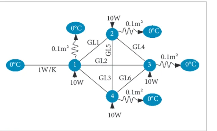
has a surface of 0.1 m² with an emissivity of 1, which radiates to the environment. 10 W are dissipated in each node. Node 1 is connected to the environment node with a thermal conductance of 1 W/K. Nodes 1 to 4 are all connected to each other by 6 thermal linear links (GL) as shown in Fig. 1.
In order for the temperatures at the nodes to correspond to the measured values, the parameter values of the thermal links need to be changed. herefore, the equation system to be solved by the algorithm is:
Tcalculated(GL) – Tmeasured = 0, (10)
where:
Tcalculated is the function which represents the model; GL is the vector containing GL1 to GL6; and
Tmeasured is the vector of the calculated temperatures for GLi = (0.1 + i/100)W/K. his is assumed to be a measurement.
The initial estimates for all GL are 0.5 W/K. Three load cases are derived from this problem: • An underdetermined system: All links are variable. here
are six parameters (links) for four values (temperatures); • A determined system: Links 3 and 6 are constant
(GL3 = 0.13W/K, GL6 = 0.16W/K). here are four parameters (links) for four values (temperatures);
• An overdetermined system: Links 3, 5, and 6 are constant (GL3 = 0.13W/K, GL5 = 0.6W/K, GL6 = 0.16W/K). here are three parameters (links) for four values (temperatures), and GL5 is chosen so that it is impossible to solve the system.
THE COMPLEX MODEL
he complex model is a model of real spacecrat hardware, which was tested in a thermo vacuum chamber. In total, 13
parameters where chosen; they consist of thermal boundary conditions, thermal conductances, and emissivities for the infrared spectrum.
Temperature readings were taken from 26 sensors at 6 test points over time, yielding 156 evaluated temperatures.
RESULTS
RESULTS OF THE UNDERDETERMINED SIMPLE MODEL
Figure 2 shows the development of the root sum square of all temperature diferences for both analyzed algorithms. he values of some signiicant points shown in this diagram are listed in Table 1. he model quickly converged toward 0, with both algorithms
0°C
1W/K 1
2
3
4
GL2
G
L
5 GL4
GL6 GL3 GL1
0°C 0°C
0°C
0°C
0.1m²
0.1m²
0.1m²
0.1m² 10W
10W
10W 10W
0 1 2 3 4 5 6 7 8 9 10 11 12 13 14 1.00E-05
1.00E-04 1.00E-03 1.00E-02 1.00E-01 1.00E+00
1.00E+01 Broy den
self -dev eloped method
Iterations after Jacobian matrix generation
RSS [K]
Figure 1. Thermal test model schematics.
Figure 2. Root sum square of the temperature differences over iterations of the underdetermined simple model.
Algorithm
Iterations for Jacobian
matrix generation
Nº of iterations after Jacobian
matrix generation
RSS/K
Broyden 6
0 (initial) 4.261
6 5.921E-03
9 2.646E-05
Self-developed
method
6
0 (initial) 4.261
6 7.652E-04
12 5.385E-05
reducing the RSS by approximately one order of magnitude every two to three iterations, until the numerical accuracy limit of 1E-5 was reached. Ater the 4th iteration, the self-developed algorithm was faster, but ater the 9th iteration, the Broyden algorithm converged faster. In conclusion, the performance of both algorithms can be considered comparable for this case.
RESULTS OF THE DETERMINED SIMPLE MODEL In the same way as shown for the underdetermined simple model, Fig. 3 and Table 2 show the root sum square development for the determined simple model. he model converged slower than for the underdetermined problem.
he Broyden algorithm needed an average of 11 steps per order of magnitude while the self-developed algorithm needed an average of only 5 of them.
RESULTS OF THE OVERDETERMINED SIMPLE MODEL
he overdetermined model converged, as expected, not to 0 but to a inite value (0.0375K), as is shown in Fig. 4 and Table 3. For this load case, the self-developed method converged considerably faster, with approximately 4 iterations per order of magnitude, while the Broyden algorithm used approximately 8 iterations per order of magnitude.
1 5 7 9 13 17 21 25 29 33 37 41 45 49 53 1.00E-05
1.00E-04 1.00E-03 1.00E-02 1.00E-01 1.00E+00
1.00E+01 Broyden
Self-developed method
Iterations after Jacobian matrix generation
RSS[K]
0 1 2 3 4 5 6 7 8 9 10 11 12 13 14 15 16 17 1.00E-02
1.00E-01 1.00E+00 1.00E+01
Broyden
Self-developed method
Iterations after Jacobian matrix generation
RSS[K]
Figure 3. Root sum square of the temperature differences over iterations of the determined simple model.
Figure 4. Root sum square of the temperature differences over iterations of the overdetermined simple model.
Algorithm
Iterations for Jacobian
matrix generation
Nº iterations after Jacobian
matrix generation
RSS/K
Broyden 4
0 (initial) 3.442
6 1.024
41 9.487E-05
Self-developed
method
4
0 (initial) 3.442
6 5.813E-02
22 1.414E-05
Table 2. Selected points of the algorithm convergence of the determined simple model.
Algorithm
Iterations for Jacobian
matrix generation
Nº iterations after Jacobian
matrix generation
RSS/K
Broyden 3
0 (initial) 3.442
4 1.869
15 3.760E-02
Self-developed
method
3
0 (initial) 3.442
4 1.869
8 3.757E-02
RESULTS OF THE COMPLEX MODEL
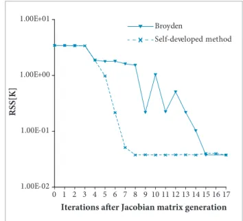
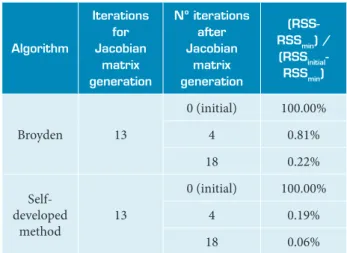
Figure 5 and Table 4 show the convergence of the algorithm for the complex model in a diferent way to the way that was shown for the simple model. he complex model is an overdetermined system and it is not expected to converge to 0. herefore, the diference between the RSS of each iteration and the best RSS reached is used. his diference is standardized to the initial value. he best RSS was reached by restarting the algorithm near the optimum.
As can be seen in the following figure, the optimum is nearly reached after a few iterations. In this steep initial part, both algorithms required approximately 2 iterations, on average, to reduce the target value by one order of magnitude.
After reaching 0.25%, the Broyden algorithm stayed stable while the new algorithm converged slowly to a lower value.
DISCUSSION OF THE RESULTS
Both algorithms converged in all of the studied cases until either the numerical accuracy limit or a limit due to an over-constrained system was reached. The number of iterations can be approximated by the formula:
m = 1 + k + r * c (11)
where:
m is the total number of iterations including the irst;
k is the number of parameters (iterations of Jacobian matrix generation); and
r is a value specific to the problem; it depends mainly on the nonlinearity of the model and the interactions between the parameters. he total number of parameters is not very signiicant for this value. For the load cases studied, the value was between 2 and 10, on average, until a certain limit was reached. For similar load cases, it is not expected to increase signiicantly; c is the desired reduction in the order of magnitude of the diference of the root sum square and the minimal possible root sum square. It is deined by the following formula:
c = log10(R0 – Rmin) – log10(Rfinal – Rmin) (12)
where:
R0 is the initial root sum square of the deviation vector (F(po) – tmes);
Rfinal is the final root sum square of the deviation vector (F(pfinal) – tmes); and
Rmin is the minimum possible root sum square of the deviation vector (F(pfinal) – tmes).
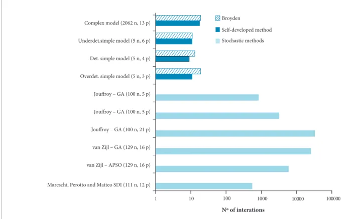
As can be seen in Fig. 6 the number of iterations needed for the presented algorithms (10 to 30) to the typical number of iterations needed for genetic (25600 (van Zijl, 2013), 843 to 33072 (Joufroy, 2007)), adaptive particle swarm optimization (6000 (van Zijl, 2013)) or the stochastic design improvement (555, (Mareschi et al., 2005)), this approach is much faster. he number of parameters of the models used in these evaluations is comparable to the complex model used in this paper, but the
0 1 2 3 4 5 6 7 8 9 10 11 12 13 14 15 16 17 18 0.01%
0.10% 1.00% 10.00% 100.00%
Broyden
Self-developed method
Iterations after Jacobian matrix generation
(RSS-RSSmin)/(RSSinitial-RSSmin)
Figure 5. relative root sum square of the temperature differences over iterations of the complex model.
Algorithm
Iterations for Jacobian
matrix generation
Nº iterations after Jacobian
matrix generation
(RSS-RSSmin) /
(RSSinitial -RSSmin)
Broyden 13
0 (initial) 100.00%
4 0.81%
18 0.22%
Self-developed
method
13
0 (initial) 100.00%
4 0.19%
18 0.06%
the number of iterations needed for the tested algorithms is 20 to 1,000 times smaller than the number of iterations reported for genetic or adaptive particle swarm algorithms. In conclusion, this algorithm signiicantly reduces the cost of a thermal model correlation.
The “good Broyden method” and the self-developed method delivered satisfactory results and are, therefore, both considered suitable. The self-developed method delivered slightly better results for most of the cases analyzed.
ACKNOWLEDGMENTS
The laser communication terminal (LCT) project, which this publication is based on, is carried out on behalf of the Space Administration of the German Aerospace Center (DLR e.V.) with funds from the Federal Ministry of Economics and Technology, under the reference number 50-YH1330. The author is responsible for the contents of this publication and gratefully acknowledges their support.
number of nodes used is considerably lower. Unfortunately, the models and tools used for these methods are not accessible so that a direct comparison was not possible.
For each iteration, the CPU time required for generating a new set of parameters is only a few milliseconds and, therefore, it is negligible compared to the minutes or hours required for solving the model. It can be concluded that the total CPU time is nearly proportional to the number of iterations, independent from the algorithm.
Both algorithms studied showed similar performance. herefore, both are considered suitable for model correlation. he new algorithm showed better performance for most situations.
CONCLUSION
It has been shown that using root inding algorithms of the Broyden class for thermal mathematical model-to-test correlation is feasible and eicient. Although a direct comparison of the analyzed methods and a genetic algorithm was not possible,
Complex model (2062 n, 13 p)
Underdet.simple model (5 n, 6 p)
Det. simple model (5 n, 4 p)
Overdet. simple model (5 n, 3 p)
Jouffroy – GA (100 n, 5 p)
Jouffroy – GA (100 n, 5 p)
Jouffroy – GA (100 n, 21 p)
van Zijl – GA (129 n, 16 p)
van Zijl – APSO (129 n, 16 p)
Mareschi, Perotto and Matteo SDI (111 n, 12 p)
1 10 100 1000 10000 100000
Broyden
Self-developed method
Stochastic methods
Nº of interations
REFERENCES
Broyden, C.G., 1965, “A Class of Methods for Solving Nonlinear Simultaneous Equations”, AMS Mathematica of Computation, Vol. 19, No. 92, pp. 577-593. doi: 10.1090/S0025-5718-1965-0198670-6.
De Palo, S., Malost, T. and Filiddani, G., 2011, “Thermal Correlation of BepiColombo MOSIF 10 Solar Constants Simulation Test”, 25th
European Workshop on Thermal and ECLS Software.
Harvatine, F.J. and DeMauro, F., 1994, “Thermal Model Correlation Using Design Sensitivity and Optimization Techniques”, 24th International Conference on Environmental Systems and 5th European Symposium on Space Environmental Control Systems.
Jouffroy, F., 2007, “Thermal model correlation using Genetic Algorithms”, 21st European Workshop on Thermal and ECLS Software.
Mareschi, V., Perotto, V. and Gorlani, M., 2005, “Thermal Test Correlation with Stochastic Technique”, 35th International Conference on Environmental Systems (ICES).
Momayez, L., Dupont, P., Popescu, B., Lottin, O. and Peerhossaini, H., 2009, “Genetic algorithm based correlations for heat transfer calculation on concave surfaces”, Applied Thermal Engineering, Vol. 29, No. 17-18, pp. 3476-3481. doi: 10.1016/j. applthermaleng.2009.05.025.
Roscher, M., 2006, “Genetische Methoden zur Optimierung von Satelliten Thermalmodellen bei EADS ASTRIUM“, Hochschule Wismar & EADS Astrium.
van Zijl, N., 2013, “Correlating thermal balance test results with a thermal mathematical model using evolutionary algorithms”, Faculty of Aerospace Engineering, Delft University of Tecnology.