A comparison of risk aversion between markets

(1)

A Comparison of Risk Aversion between Markets

José Tavares

Student no. 152111141

Advisor:

Professor Joni Kokkonen

This dissertation is submitted in partial fulfilment of the degree of IMSc in Business

Administration, September 16, 2013

(2)

(3)

iii

Abstract

In this study we perform a comparison between the Dow Jones Industrial Average and the FTSE 100 indexes concerning their estimated risk aversions. Risk neutral densities are calculated for both indexes using a polynomial-lognormal, a GB2 and a mixture of two lognormal distributions; we show that the best fit to observed data is obtained using the latter. For the method of best fit, and assuming a power utility function, the risk aversion of investors is calculated using a maximum likelihood method and a likelihood ratio. The FTSE 100 presents the highest value of risk aversion of the two indexes, as well as the lowest volatility. A negative correlation is found between risk aversion estimates and the volatility of the underlying index.

Keywords: Lognormal Mixture; Generalised beta; Hermite Polynomials; Risk Neutral Densities;

(4)

iv

1 - Introduction

In finance, knowing future density forecasts of stock prices, commodity prices, exchange rates or interest rates has a critical importance to many economic agents and decision-makers. Recently, with the spread of option markets, new methodologies have been advanced that allow the forecast of price densities as well as estimations of the market's level of risk aversion by using the information contained in option prices. Option forecasts are often demonstrated to provide added accuracy compared to historical analysis in the calculation of both volatility and probability density functions (Liu, et al., 2007). Most contributions in these areas are concerned with testing the methods and their ability to create good forecasts. This study, however, will focus more on the conclusions that can be drawn from the market by using the methodology, namely a comparison between risk aversions in two different markets.

More than just an expected value and a volatility measurement, densities provide probabilities for each level of future prices and allow further measurements such as skewness and kurtosis. One of the main consumers of this kind of information are central banks. As major regulatory institutions, central banks are interested in the density predictions of interest rates, exchange rates, commodity price levels and stock indexes. This allows them to know more about the economic expectations of investors, the confidence in the markets, the expected corporate earnings reflected in the index levels, as well as how to best establish the short-term interest rates in the money market (European Central Bank, 2011) (Shackleton, et al., 2010).

Learning about the expectations of investors is a two step process that will be covered in this dissertation. First, using the option prices, we will estimate the risk neutral density, a probability distribution that assumes the risk neutrality of investors. Out of all the parametric and non parametric methods that can be used, we will test three well known parametric methods to determine which one best follows the information present in the option prices. Next we will use two different methods to calculate an estimation of the risk aversion of investors. Using this estimation and assuming a power utility function, it is possible to transform the risk neutral density into a real world density that corresponds to the actual expectations of investors.

The purpose of this dissertation is to estimate the risk aversion in the U.S. market and compare it to the risk aversion estimated for the U.K. market in the period before the financial crisis of 2008 to capture the estimates of risk aversion under normal market conditions. To do so, the two-step process just described will be performed in parallel for option data coming

(6)

2

from options on the Dow Jones Industrial Average index and on the FTSE 100 index between October 2006 and June 2007.

We find that both methods to estimate risk aversion suggest higher values for the FTSE 100 than for the Dow Jones Industrial Average. In an attempt to explain these results, we conclude that the risk aversion estimate presents a negative correlation to the market volatility; findings that are in line with the paper by Bliss and Panigirtzoglou (2004). Furthermore, the volatility defined as the coefficient of variation of the Down Jones Industrial Average is higher than that of the FTSE 100 for the period analysed, which may be behind the lower risk aversion estimate found for the American index.

Section 2 of this dissertation will cover the most common methods to estimate the risk neutral densities and the real world densities, referring to publications of high academic worth. Section 3 describes in more detail the methodology used in this dissertation; section 4 presents the results along with some explanations and section 5 summarises the findings.

2 - Literature Review

2.1 - Historical methods

One way to estimate the density functions is through the analysis of past returns. In that case, a time series of the prices of the asset being studied is collected, returns are calculated and usually a model is chosen to try and explain the observed data. There are several models that can be used, some of the most common ones belonging to the ARCH family which has applications for all the different classes of assets. ARCH models are defined by conditional densities, i.e. distributions of returns for a given time are conditional on previous returns. More notably, the conditional variance of the model recognises the existence of volatility clustering and reflects this heteroskedasticity on the estimation of return distributions. These models will have a set of parameters which are estimated through the maximisation of a likelihood function. This means that the parameters will ensure the best fit of the model to the historical data collected. The likelihood analysis itself is also an important part of determining the best model for a particular set of data. (Taylor, 2005)

2.2 - Option-based methods

Another alternative to learn about densities of future prices of a given asset is to analyse the prices of options that have that asset underlying. It is a valid source of information since the price at which options are being transacted has a "forward-looking nature" and contains clues regarding the perceptions of the market for the price of the asset in the future (Bahra, 1997). For many years the inexistence of a sufficient number of exchange traded options limited the information that could be extracted from option prices, and so the empirical research that has been done on the subject is quite recent (Jackwerth, 1999) (Jackwerth, 2004). Approaching the end of the century, however, the spread of option trading led to the availability of several

(7)

3

option prices for all kinds of assets, for different maturities and different exercise prices. This availability of different contracts made option prices a major source of information in finance. According to Bliss and Panigirtzoglou (2004), one big advantage of distributions extracted from option prices over those extracted from time series is that the information comes from one single point in time, and the fact that the distribution doesn't depend on the past information makes it more responsive to changes in the market. Furthermore, the authors support that the existence of a predetermined expiration date, as well as the different investment horizons for which option prices are available permit the study of both specific horizons and multiple horizons.

2.3 - Risk Neutral Densities

To extract a density from the prices of options it is possible to use merely the prices of call options. This happens because of the put-call parity. Since there is a link between the prices of the two types of options, the utilisation of a second type of options would be unnecessary (Taylor, 2005).

The density that is extracted directly from the prices of options without any kind of risk transformations is called a Risk Neutral Density (RND). This means that the density obtained is the real density only for risk neutral investors. Since it is commonly assumed that investors have some degree of risk aversion, further calculations will have to be performed at a later stage to ensure a credible real density function.

The techniques used to extract RNDs from option prices trace back to the studies of Breeden and Litzenberger (1978). They show that the prices of primitive securities1_{can be obtained}

from the prices of call options and, since the prices of primitive securities are related to the probability of the underlying assuming a given state, there is a direct link to calculating the RND. The authors build a primitive security from four call options with exercise prices spaced by ∆M forming a butterfly spread centred in M. They then demonstrate that the limit of the pricing function of this security is

whenever ∆M tends to zero, where C is the price of the call option and with the strike price X equal to the state M. This result tells us that the second derivative of an option pricing formula with respect to its exercise price X gives the discounted density of the underlying asset.

The next step is to find a way to describe the observed prices of options using a formula that can be derived twice with respect to the strike price. Given that the construction of an RND would require a continuous set of option prices and that the market only provides option prices for discrete values of X and for a limited range of X, it is necessary to both interpolate between the strike prices for which there are observations and to extrapolate out of the range of available strike prices to obtain information about the tails of the distribution (Bahra, 1997). The methods to do so can initially be divided into parametric and non-parametric. These two groups will be discussed in more detail in the next sections.

(8)

4

2.3.1 - Parametric Methods

Parametric methods, as indicated by the name use functions of price that are shaped by only a few parameters that are optimised to make the call prices calculated by the formula fit the prices observed in the market. The maximisation of the fitness is usually achieved by the minimisation of the sum of the squared errors between the prices given by the formula and the observed prices (Taylor, 2005). According to Jackwerth (1999), parametric methods can be divided into three categories: expansion methods, generalised distribution methods and mixture methods. Expansion methods start from a simple density shape, such as the lognormal and introduce extra flexibility by adding a correction term. A common example of such a distribution would be a lognormal-polynomial density like the one used by Corrado and Su (1997). The authors analyse S&P 500 index option prices and criticise Black and Scholes's (1973) assumption of lognormality in stock price distributions. Their suggestion is an expanded version of the model, which allows flexibility in the values of skewness and kurtosis and which effectively manages to flatten the volatility smile2_{, thus showing improved}

accuracy. This method, however, is known for sometimes providing negative values for the RND making it important to carefully evaluate its results (Jackwerth, 1999).

Generalised distribution methods use models that incorporate more parameters than a lognormal distribution, thus displaying more flexibility and a better fit to the data. Bookstaber and McDonald (1987) introduced generalised beta functions of the second kind (GB2), a four parameter function, "as a descriptive tool rather than as a definitive distribution" (Bookstaber and McDonald, 1987, p. 419). This distribution embeds other distributions such as the lognormal, the log-t and the log-Cauchy as limiting cases or special cases and has the advantage of being extremely flexible. Taylor (2005), defends that the distribution is easy to calculate and doesn't tend to return negative values for the density like a lognormal-polynomial, its biggest problem being the interpretation of some of its parameters.

Lastly, mixture methods have as typical example the mixture of lognormal density functions. These simply make a distribution from a weighted average of two or more lognormal distributions. The final distribution will have two parameters for each lognormal used (mean and variance) as well as one or more parameters for the weights. The number of parameters will be 3n-1, with n being the number of lognormal densities used. This leads us to the method's drawback of easily accumulating a large number of parameters when the amount of lognormal densities increase. A mixture of more than two lognormals can also incur in the problem of overfitting the data (Jackwerth, 1999). Generally, however, this model is quite flexible and is especially suited for cases where there are two possible distinct states in the economy, which can even lead to a bimodal distribution (Bahra, 1997). Ritchey (1990)

2_{The volatility smile consists of the representation of implied volatilities (volatilities calculated by}

reversing a given option pricing formula so that it provides a volatility when an observed price is inputted) at different strike prices. As the volatility refers to the underlying asset, it should be constant regardless of the strike price of the option contracts associated. However, the wrong assumption of lognormality in the future prices of the underlying asset leads to an implied volatility representation that is higher for very in the money and out of the money exercise prices; an illustration that resembles a smile and which earned it the name.

(9)

5

suggests using a mixed lognormal rather than the regular Black-Scholes model, claiming that the latter was mispricing options especially in out of the money near expiration options with high kurtosis and high positive skewness of underlying returns. Using a sum of weighted Black-Scholes solutions is a more accurate alternative.

2.3.2 - Non-Parametric Methods

Non-parametric models are different from the ones discussed above in the way that they make no assumptions and impose no parametric restrictions regarding the form of the density, the pricing formula or the process of the returns (Bahra, 1997). Instead, they try to fit the option prices in a more general way by presenting no rules regarding the possible shape of the density, which usually makes them very flexible. They sometimes also incur the problem of overfitting the data, meaning that they respond too quickly and are too sensitive to individual observations. This can prove to be a problem when there is noise in the observations or mispricing in one of the securities because the overall pricing function estimated can become compromised. The non-parametric methods can again be divided into three other groups: kernel methods, maximum entropy methods and curve fitting methods (Jackwerth, 1999). Kernel methods assume that each observed data point is in the centre of a distribution and that the likelihood of having the real function pass through a given point depends on the distance between that point and the observed data point (Jackwerth, 1999). Aït-Sahalia and Lo (1998), for example, use a kernel-type method and argue that, while parametric methods are simpler and less data-intensive, non-parametric ones are not restricted by assumptions that may not hold true. This, according to the authors, makes them more robust.

Maximum entropy solutions are those that minimise the commitment to unknown information. They can incorporate many constraints into the distribution and assume maximum uncertainty for the information that is missing. Buchen and Kelly (1996) use the principle of maximum entropy to extract the distribution of an asset from option prices. The authors support that, from a statistical inference standpoint, this is the best method since it complies with all the restrictions inputted, such as the observed prices of options, and provides the least prejudiced density in the sense that it assumes as little as possible.

The curve fitting group encompasses a broad number of methods from polynomials to splines. Jackwerth and Rubinstein (1996) fit a curve to observed S&P 500 option prices to extract a risk neutral distribution. They use a new technique that maximises the smoothness of the distribution while still meeting the points of the observed option prices. They also report a difference in the skewness and kurtosis of the RND of the index before and after the 1987 market crash.

2.3.3 - Implied Volatility Methods

The methods covered above all aim at fitting the pricing function to the observed prices. An alternative technique can be used by specifying the implied volatilities' curve instead of the curve of option prices. To do so both parametric and non-parametric methods can be used. Shimko (1993) applied a parametric method using quadratic polynomials to fit the curve of implied volatilities. The author could then use the resulting volatility function to calculate the

(10)

6

option pricing function and obtain the RND. It is, however, difficult to extrapolate the implied volatility function to obtain values outside the defined strike price range, and so Shimko had to use the tails of lognormal distributions and attach them to his calculated density. Malz (1997) also used quadratic polynomials but he chose to fit that formula not to volatilities in a scale of strike prices but in a scale of option deltas, which proves useful in defining the tails of the distribution but complicates the translation of the scale back to strike prices (Taylor, 2005) (Jackwerth, 2004).

2.4 - Real World Densities

Especially for equity densities, one shouldn't rely on the RND without any kind of risk transformation since the neutral densities ignore the effects of risk aversion which, for this asset type, can be quite significant (Shackleton, et al., 2010). It has been suggested in a number of studies that a density directly extracted from option prices is a poor predictor of the future distribution of the underlying asset. If it is to be assumed that investors are rational, the difference between the RND and the real density must be explained by risk aversion and thus, by comparing the two densities, it would be possible make conclusions about the risk preferences of the general market. This assumption is widely supported by a number of studies that point towards the existence of a risk premium particularly evident in equity prices (Mehra and Prescott, 1985) (Bliss and Panigirtzoglou, 2004).

The estimated RND and the real density are related by a given utility function. According to Bliss and Panigirtzoglou (2004), if we take the RND, q(ST), the real world distribution, p(ST),

and the utility function, U(ST), the following condition holds:

(1)

where St is the price of the asset at observation, ST is the price of the asset at expiration, is a

constant and the right side of the equation is equivalent to the pricing kernel. As such, both densities and the utility function are related in such a way that, knowing two of them makes it possible to calculate the third. Two commonly assumed utility functions are the exponential utility defined as _{which presents a constant absolute risk aversion and the} power utility function that follows

(2)

(11)

7

Some authors like Aït-Sahalia and Lo (2000), after estimation of the RND, choose to obtain the objective density function3 from a historical analysis of the underlying assets' time series and

then use these two densities to calculate the utility function. This presents a strong assumption that there is stationarity in the real distributions. Other authors even extend this assumption of stationarity to the risk neutral density. Bliss and Panigirtzoglou (2004) don't agree with these assumptions and claim that they produce risk aversion functions that are inconsistent with theory. To them, the assumption to be made is that of a stationary utility function for the duration of the sample. Bliss and Panigirtzoglou then test the ability of an estimated density to forecast the true density. They use a variable ST which is the price

realisation of the underlying asset at the maturity of each option observation and claim that, assuming that ST are independent and that the estimated density is equal to the true

density, the variable such that

(3)

is independent and identically distributed (i.i.d.) following a standard uniform distribution. Confirmation of these assumptions would mean the estimated density is in fact the true density. The authors then use the methodology proposed in Berkowitz (2001) as a joint test to check whether these assumptions hold. Berkowitz defines a new variable such that

₍₄₎

where _{represents the inverse of the standard normal cumulative distribution and states} that is i.i.d. and follows a standard normal distribution whenever the estimated density is the same as the true density. The model

(5)

is created to test and (mean of zero and variance of one as required by the standard normal as well as no correlation to ensure independence). The model's parameters are estimated by maximising the log-likelihood function:

3_{The objective density is considered to be the real distribution followed by the price realisations. This}

distribution is closely approximated on average by the real expectations of investors, assuming they are rational.

(12)

8 (6)

From this likelihood it is possible to test the independence with

(7)

following a chi-square with one degree of freedom and to jointly test independence and standard normal distribution using

(8)

which follows a chi-square with three degrees of freedom. The value of the risk aversion that leads to the minimum should be selected, since it reduces the chances of rejection of the null hypothesis. In other words, it maximises the possibility of being an i.i.d variable following a standard normal, which only happens when the estimated density is the real one. The becomes important to understand a possible joint test rejection. When that happens, a rejected suggests that there is a problem with the independence of the variables (as may happen if the periods under analysis are overlapping) which makes the test inconclusive.

Liu, et al. (2007) disagree with this method and claim that, while there is important diagnostic value in the LR3 method, they have no knowledge of the method being superior to a maximum

likelihood estimate of the risk aversion as far as accuracy is concerned. The authors use a power utility function with a CRRA of and a marginal utility of _{. The RND is defined as} and the real world density as . The real world transformation is thus performed by using:

(9)

where the integral is a constant adjustment factor used to ensure that the transformed density still integrates to one. The variable y is chosen to make sure that is not present in the denominator, which would keep it from being constant.

A different way to estimate the real density than assuming a utility function is by using a recalibration function. Liu, et al. (2007) give preference to a calibration method followed by Fackler and King (1990) which uses a beta transformation. The calibration function for this method is the cumulative distribution function for a beta distribution:

(13)

9

where j and k are the calibration parameters. Defining as the cumulative distribution function of a risk neutral density, the link between the real world density and the RND comes from

(11)

To estimate the transformation parameters (either or (j,k)), the log-likelihood function

(12)

should be maximised.

Literature about this topic presents a very diverse set of values for . For a power utility function, Bliss and Panigirtzoglou (2004) estimate the parameter for different maturities of the option contracts and for different volatilities. Their results range from just under 1 for 6-week expiring options with high volatility to above 12 for options expiring in one 6-week and low volatility. Liu, et al. (2007) estimate a lower value of 1.85 when using a mix lognormal method, but claim that their result is lower than expected due to a market decline taking place during the time of their analysis. Others authors like Cochrane and Hansen (1992) suggest that may be in excess of 40.

3 - Empirical Methods

3.1 - Data

Data have been extracted from Wharton Research Data Services (WRDS) for the call prices of the Dow Jones Industrial Average representing the American market and of the FTSE 100 representing the UK. The option prices were recorded for the 5th of October 2006 with a maturity of 11 trading days (21st of October 2006). Within these dates, 33 observations were collected across the range of strike prices for the Dow Jones Industrial Average and 19 were found for the FTSE 100. For the purpose of estimating the risk aversion, 8 extra densities representing each month until June of 2007 were extracted from WRDS. This database was also used to obtain the closing prices and the dividend yield of both indexes at the option's

(14)

10

observation date. The risk-free rate considered was the three-month Eurocurrency interest rate4. The option prices considered for analysis are an arithmetic average of the bid and ask

prices for each day.

In order to calculate the RND implied by the observed call prices, parametric methods shall be used since, as previously seen, they are less data-intensive and provide a more independent view of the curve by not overfitting the data. It is important, at this stage, to compare some of the methods from the different categories discussed before.

3.2 - Risk Neutral Densities

3.2.1 - Expansion method

For this category, a lognormal-polynomial density using normalised hermite polynomials will be applied. As previously seen in the literature review, this method assumes a lognormal distribution to which is multiplied a polynomial that brings flexibility to the distribution and contributes to the definition of the skewness and kurtosis which are not accounted for with the simple lognormal. The normalised hermite polynomials that are multiplied in the density function follow the denomination , with the first order polynomials being:

(13)

These polynomials have the orthogonality property, which means that the integral will be 1 whenever and zero otherwise. The density distribution of Z, a random variable with mean of zero and standard deviation of one comes from:

(14) where (15)

and are the parameters to be estimated. Additionally, it is known from theory that is 1 and both and are zero. It will also be assumed that the values of with an index higher

4_{Interest rate earned by deposits made by governments and corporations in foreign banks. The}

three-month rate is the most liquid one and, as such, considered a good approximation of the risk free interest rate.

(15)

11

than 4 are equal to zero. These values will be needed to calculate the pricing function of the options, as:

(16)

where comes from calculating

(17) and so: (18)

(16)

12

The formulae for and need not be calculated since their multiplication with the null values of and will eliminate them in the product. We then have the optimisation of the parameter vector done by minimisation of the sum of square errors

(19)

which compares the option prices obtained using the model ( ) with the ones observed in the market ( ) and where is the number of strike prices for which there are observable prices. The lowest value of happens for parameter values that best fit the model to observed data. Finally, the density function of the future stock prices is linked to the density of (defined in Equation (15)) by the expression:

(20)

3.2.2 - Generalised distribution method

The method being used here will be one of the most common ones, the GB2 originally used by Bookstaber and McDonald (1987). This distribution has four parameters defined as to ensure flexibility and description of values of skewness and kurtosis. It is however useful to define parameter b as a function of the other three parameters to force a risk neutrality condition for the final distribution. The fact that these parameters are difficult to interpret is one of the drawbacks of this method. The probability density function is defined as:

(21)

where the beta distribution is defined by

, with the gamma function being easily calculated by a Microsoft Excel formula. The parameter b, as previously said, comes from a function of the other parameters as

(22)

Before writing the option pricing function, it is necessary to define the cumulative distribution function of the beta distribution

(17)

13

(23)

where the function u is a result of

(24)

The pricing formula is then:

₍₂₅₎

3.2.3 - Mixture method

A simple but effective method in this category is the mixture of two lognormal distributions. As previously discussed, this method allows a higher degree of flexibility than the simple lognormal, permitting the description of several measures of kurtosis and skewness. It can even account for bimodal distributions, a useful feature when there is a marked doubt between two possible states in the market. Each lognormal density must have one parameter for the mean and another one for the volatility. A fifth parameter is the weighting of the lognormal distributions in the final RND. Therefore, . Since the equality must hold5_{, only four parameters need to be optimised. The density for}

each of the lognormals follows:

(26)

with and d2 coming from Black and Scholes (1973):

(27)

The RND, being a weighted average, is:

(28)

(18)

14

and the pricing formula is the weighted average of two pricing formulae equal to the one found in Black and Scholes (1973):

₍₂₉₎ where .

3.3 - Risk Transformation

3.3.1 - Maximum Likelihood

As stated before, given the common assumption of risk aversion in the market, an RND is close to useless when it comes to forecasting the future prices of an underlying asset. As such, it is now necessary to perform a risk transformation to obtain a real world density. Since it can be seen in the results' section that the mixture of lognormals method seem to best explain the pricing of options for both indexes, we shall use the RNDs calculated with it to perform the risk transformation. For this risk transformation, it will be assumed that the risk neutral densities are linked to the real world densities by a power utility function, which implies a constant relative risk aversion . Additionally, following Liu, et al. (2007) where they claim that the LR3 method is not known by them to produce a more accurate estimation of the risk aversion factor , the maximum likelihood shall be used as the main estimation method. To increase the accuracy of the method, nine sets of option prices have been collected, with the first set having its option prices observed at October 5th_{2006 and expiry date at October 21}st

2006 (the same set used to calculate the RNDs). The remaining data sets are all concerning options with the duration of two weeks and the observation dates are in the beginning of each of the months following October until June. For each of these data sets, densities are calculated the same way as described in the RND section above. Then, using the transformation shown in Equation (9), the transformed parameters are calculated as:

_and

(30)

where are the set of transformed means for each of the lognormal densities and is the transformed weight.

Creating a probability density function the same way as done before, but now using the transformation parameters will result in a real world density, the purpose of this exercise. However for the transformation to be possible, one more parameter must be estimated. That parameter is the risk aversion measurement that is present in the above formulae of the transformed density parameters and and that also defines the assumed power utility

(19)

15

function To estimate the parameter it is necessary to maximise the log-likelihood function of the observed prices at the end of each of the nine periods given the transformation parameters which depend on the risk aversion parameter. In other words, a value of must be chosen in such a way that the probability of the observed end-of-period index levels coming from the transformed parameters is maximal. In practical terms, this can be done simply by maximising the sum of the logarithms of the transformed density function at each of the end-of-period index prices. Mathematically: .

3.3.2 - LR3

To reinforce the conclusions regarding the risk aversion for the two indexes under analysis, we will now use the LR3 method proposed by Berkowitz (2001). For the same nine real world densities previously estimated by the maximum likelihood method, a close approximation of their integral was performed by dividing the strike price range into multiple sections. Each of these sections is represented by a density value and, by multiplying these values by the width of the section and summing the resulting products we obtain the area beneath the density curve; in other words, the integral. The integration from minus infinity until ST as can be seen

in Equation (3) returns a variable that follows an i.i.d. distribution if the estimated density is the same as the true density and ST are independent. Application of the Equation

(4) to variable originates variable which should be i.i.d. and follow a standard normal distribution. This procedure is performed for both indexes being analysed and two sets of nine values of are obtained. Maximising the log-likelihood displayed in Equation (6) produces estimates for the parameter vector obtaining the remaining information needed to perform the calculation of and (Equations (7) and (8)). A value for the risk aversion must now be chosen in such a way that it results in the lowest possible . Doing so will maximise the chances of being independent and defined by a standard normal and so, having a correctly specified real world density.

4 - Results

4.1 - Risk Neutral Densities

4.1.1 - Polynomial-Lognormal

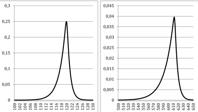
Performing the optimisation of the pricing function parameters by minimisation of defined in Equation(19) was done using solver in Microsoft Office Excel. The parameter vector for the Dow Jones Industrial Average is resulting in and the optimum for the FTSE 100 comes at . The shapes of the RNDs are as follows.

(20)

16 0 0,05 0,1 0,15 0,2 0,25 100 102 104 106 108 110 112 114 116 118 120 122 124 126 128 130

We observe that the peaks are at around 119.2 for the Dow Jones Industrial average and at 604 for the FTSE 100, slightly above the respective current index levels since the time to maturity is close to 2 weeks and a high appreciation of the index would be unlikely. Given that this method can sometimes originate distributions with negative probabilities for some values of the strike price, there has also been a verification regarding the sign of the density function which, for the Dow Jones Industrial Average, appears to be positive across the range of considered exercise prices. However, it should be noted that the positive density restriction is not met by this model in the case of the FTSE 100 index. This means that the lognormal-polynomial is not adequately estimating the risk neutral density for this index. It can also be noted that the left tail of both distributions is much more significant than the right one, hinting at the higher expectations for a negative outcome than for a positive one. This trait of the probability density is usually not captured by a simple lognormal distribution, which can lead us to conclude that the inclusion of hermite polynomials added flexibility to the distribution and allowed it to display a negative skewness that is typical of stock markets. However, it is important to bear in mind that these curves are simple RNDs and no significant conclusions regarding the expectations of investors can be made until a suitable risk transformation is applied.

Figure 1 - Risk Neutral Densities for the Dow Jones Industrial Average and the FTSE 100 at October 5, 2006 using the Lognormal-Polynomial expansion method.

-0,005 0 0,005 0,01 0,015 0,02 0,025 0,03 0,035 480 490 500 510 520 530 540 550 560 570 580 590 600 610 620 630 640

(21)

17 0 0,05 0,1 0,15 0,2 0,25 0,3 100 102 104 106 108 110 112 114 116 118 120 122 124 126 128 130 4.1.2 - GB2

Once again, the parameters are estimated by minimising the error measurement (Equation (19)) using solver in Excel, which gives an optimal result of for the Dow Jones Industrial Average and for the FTSE 100. The RNDs plotted against exercise prices can be seen below.

These distributions present high peak around prices 119.9 and 612 that could imply a higher expectation for the future prices of the underlying assets assuming those values as if the investors were risk neutral. To both sides of the peak, the curves are smooth, descending more slowly on the left side. Also for this method can negative skewness be observed.

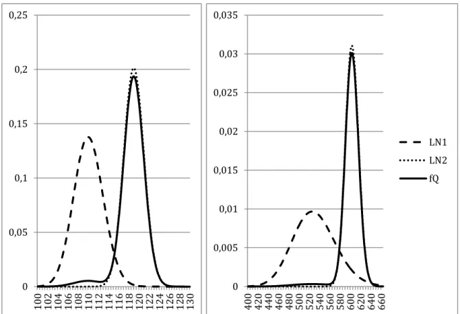
4.1.3 - Mixture of Lognormals

Again, by minimisation of the error measurement , the parameters are estimated, with resulting in a measure of error of 0.0153 for the distribution of the future levels of the Dow Jones Industrial Average. The

same calculations applied to the FTSE 100 index produce

For these parameters, both lognormal curves and the RNDs assume the following shapes:

0 0,005 0,01 0,015 0,02 0,025 0,03 0,035 0,04 0,045 500 510 520 530 540 550 560 570 580 590 600 610 620 630 640 650

Figure 2 - Risk Neutral Densities for the Dow Jones Industrial Average and the FTSE 100 at October 5, 2006 using the GB2 method.

(22)

18

We can clearly observe the two lognormal distributions that give origin to the final RND. The first lognormal expects a significantly lower distribution of the underlying index level but, as can be understood by the values of p under 4% and by the weighted distributions, an hypothetical event that would lead to these distributions is extremely unlikely. In fact, these low values of p raise doubt on whether there is really a two-state expectation for the future or if the lognormal 1 is formed merely to create a fatter left tail in the RND. It is common to come across RND shapes for this method with a similar appearance. In Liu, et al. (2007), the exemplified density created with a mixture of lognormals presents no indications of bimodality, which implies a low weight for one of the lognormal densities or a small difference between and .

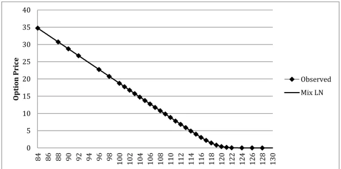
What also jumps to attention by analysing Table 1 and Table 2 is the fact that this method achieved the best fit to observed prices of all the three methods tested. If we compare the Dow Jones Industrial Average option prices observed in the market with the ones obtained from the calculated pricing formula using the mixture of lognormals, the following plot can be drawn. 0 0,005 0,01 0,015 0,02 0,025 0,03 0,035 400 420 440 460 480 500 520 540 560 580 600 620 640 660 LN1 LN2 fQ 0 0,05 0,1 0,15 0,2 0,25 100 102 104 106 108 110 112 114 116 118 120 122 124 126 128 130

Figure 3 - Risk Neutral Densities for the Dow Jones Industrial Average and the FTSE 100 at October 5, 2006 using the Mixture of Lognormals method. Both lognormal distributions that comprise the RND are represented in a dotted line and their weighted average is the solid line named fQ.

(23)

19 0 5 10 15 20 25 30 35 40 84 86 88 90 92 94 96 98 ₁₀₀ ₁₀₂ ₁₀₄ ₁₀₆ ₁₀₈ ₁₁₀ ₁₁₂ ₁₁₄ ₁₁₆ ₁₁₈ ₁₂₀ ₁₂₂ ₁₂₄ ₁₂₆ ₁₂₈ ₁₃₀ O p tio n Pri ce Observed Mix LN

In Figure 4 we can observe how the function is tracking the observed prices and how the interpolation fills in the spaces between the existing observed data.

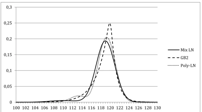
Placing all three distributions in the same graph to facilitate comparison and analysis results, for the Dow Jones Industrial Average distributions, in the chart below.

Figure 4 - A pricing formula using a Mixture of Lognormals represented with observed call prices against exercise prices at October 5, 2006 for the Dow Jones Industrial Average.

(24)

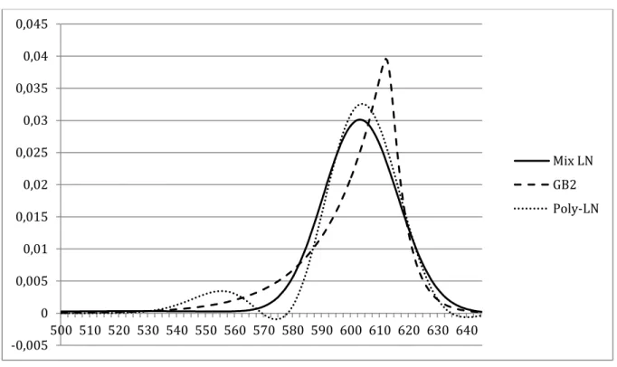
20 0 0,05 0,1 0,15 0,2 0,25 0,3 100 102 104 106 108 110 112 114 116 118 120 122 124 126 128 130 Mix LN GB2 Poly-LN

It is immediately evident the pronounced peak displayed by the GB2 method as well as an apparent stronger negative skewness. The polynomial-lognormal shows a bimodal distribution by featuring a second peak on the left slope. It is to be noted, nevertheless, how similar the three densities are on the right slope, all seeming to converge. The first four moments of the distributions and their fit to observed prices can be summarised as follows.

Mix LN GB2 Poly-LN Mean 118.64 118.80 118.81 Standard Deviation 2.70 2.63 2.48 Kurtosis 4.94 3.26 1.79 Skewness -1.50 -1.13 -0.74 G(θ) 0.015 0.019 0.021

Table 1 - Comparison of the characteristics of Risk Neutral Densities obtained with each of the three methods analysed at October 5, 2006 for the Dow Jones Industrial Average.

The mean values for the three methods seem to converge presenting a very low difference between them. It is also made obvious the negative skewness of all densities, which succeed in capturing the larger relevance of the probability in the left tail of the distribution that is common for equity densities. The higher peak of the GB2 distribution, however is not

Figure 5 - A comparison of Risk Neutral Densities calculated with each of the three methods analysed at October 5, 2006 for the Dow Jones Industrial Average.

(25)

21

confirmed by the kurtosis measurements where the generalised method trails the mixture of lognormals' produced density.

However informative each of the distributions may be, preference shall be given to those with a higher fit to observed option prices, by other words, the methods with the lowest . In this case, the mixture of lognormals and the GB2 seem to be superior to the polynomial-lognormal, with values of 0.0153 and 0.0191 against 0.0214 respectively.

Performing the same analysis for the FTSE 100, we get:

Figure 6 - A comparison of Risk Neutral Densities calculated with each of the three methods analysed at October 5, 2006 for the FTSE 100.

Mix LN GB2 Poly-LN Mean 601.22 601.04 600.32 Standard Deviation 19.41 18.67 17.57 Kurtosis 16.43 109.76 3.34 Skewness -2.95 -4.57 -1.68 G(θ) 0.361 2.901 2.967

Table 2 - Comparison of the characteristics of Risk Neutral Densities obtained with each of the three methods analysed at October 5, 2006 for the FTSE 100.

-0,005 0 0,005 0,01 0,015 0,02 0,025 0,03 0,035 0,04 0,045 500 510 520 530 540 550 560 570 580 590 600 610 620 630 640 Mix LN GB2 Poly-LN

(26)

22 0 0,05 0,1 0,15 0,2 0,25 103 104 105 106 107 108 109 110 111 112 113 114 115 116 117 118 119 120 121 122 123 124 125 126 127 f(x) f ̃(x)

For this index, it seems that each of the distributions retains some of their distinctive features, while at the same time magnifying them. It is still observed a higher peak for the GB2 confirmed by its higher kurtosis and now, its negative skewness is even more pronounced when compared with the other distributions. The polynomial-lognormal is still characterised by its bimodal appearance, which is now exacerbated so that the probability distribution assumes negative values for some exercise prices. There seems to be an agreement concerning the means of the distributions as their differences are lower than one. Both of these distributions have worsened significantly the error measurement in comparison to the ones obtained for the Dow Jones Industrial Average estimations. Additionally we can see that now there seems to be some more discrepancies regarding the shapes produced by the different methods. This result may come from the fact that data found for the FTSE 100 index was significantly less extensive regarding the number of exercise prices available for transaction.

Unlike what was seen for the Dow Jones Industrial Average where there seems to be a small difference in the error measurement for the three methods used, for the FTSE 100 it is clear that the Mixture of Lognormals’s method outperforms the other two by providing a superior fit.

4.2 - Real World Densities

4.2.1 - Maximum Likelihood

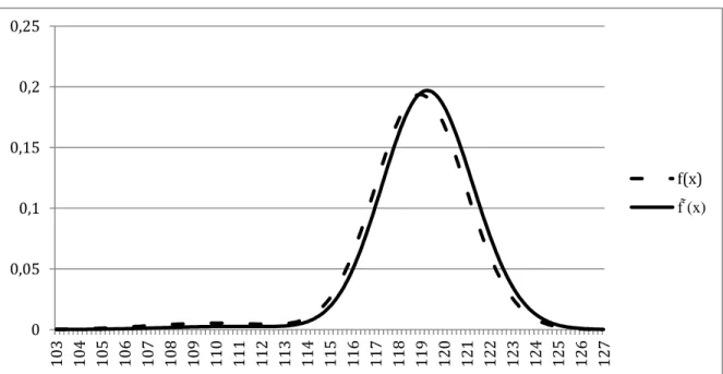
The optimisation process applied to the data collected for the Dow Jones Industrial Average index results in a value of 9.39, a positive value that suggests the presence of risk aversion and risk premium. The utilisation of this parameter on the transformation procedure specified in Equation (30) results in an increase of the log-likelihood of 0.772 and has the following effect on the RND shape previously considered for the options expiring in October of 2006:

Figure 7 - The Risk Neutral Density f(x) and its transformed density f (x) assuming risk aversion at October 5, 2006 for the Dow Jones Industrial Average.

(27)

23

A slight transformation can be observed, its most distinctive trait being the shifting of the whole density to the right towards higher values. Additionally, the weight allocated to the lognormal density that represents the worst case scenario is reduced, decreasing the significance of the results in the left side tail of the distribution. This is a common result when in presence of risk aversion, with the RND displaying a more pessimistic forecast of the index values. The fact that the market is acting as if the probability density were more negative than actually expected reflects the conservative behaviour of a risk averse investor.

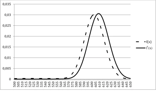
Performing the same procedure with the distribution of the FTSE 100 index increases the log-likelihood by 1.218 for a value of equal to 21.28. Again, for the density of options expiring in October 2006, this risk transformation has the following impact:

Figure 8 - The Risk Neutral Density f(x) and its transformed density f (x) assuming risk aversion at October 5, 2006 for the FTSE 100.

The same observations as for the Dow Jones Industrial Average can be made, with the right handed shift of the curve being even more pronounced on account of a higher measure of risk aversion. As obvious as this mean-shift may be, it is important to be aware that there are also changes taking place in the shape of the distribution and therefore the method used to perform the transformation is also relevant (Anagnou, et al., 2002).

Given the increase (measured as the difference between before and after) of the log-likelihood measurement achieved by performing the transformation, it is possible to test the null hypothesis of . For this test, the double of the improvement log-likelihood measurement follows a chi-square distribution with one degree of freedom. For increases of 0.772 and 1.218 for the Dow Jones Industrial Average and the FTSE 100 respectively, the testing statistics are

0 0,005 0,01 0,015 0,02 0,025 0,03 0,035 500 505 510 515 520 525 530 535 540 545 550 555 560 565 570 575 580 585 590 595 600 605 610 615 620 625 630 635 640 645 650 f(x) f ̃(x)

(28)

24

1.544 and 2.437, both of which fail to reject the null hypothesis at a 10% significance level. This means that these values of do not provide strong evidence to support the existence of risk premia in the market (Liu, et al., 2007).

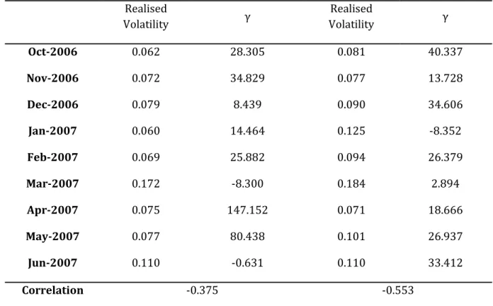
Comparing the values for the two indexes under analysis could lead to the conclusion that risk aversion is stronger for the English index. However, bearing in mind conclusions from Bliss and Panigirtzoglou(2004), estimations of the risk aversion tend to decrease with longer maturities and during periods of high volatility. The discrepancy between the values found could be explained by different volatilities felt in each market at the time of the analysed periods. Performing the optimisation of the risk aversion factor for each of the 9 periods individually brings to attention the extraordinary fluctuation existing between the values of across the different periods. While witnessing values going as low as -8 (which would suggest the existence of a risk-seeking behaviour during certain periods), it is important to bear in mind that the risk transformation procedure is merely trying to reconcile the differences between the risk neutral expectations of investors and the actual observed index levels at the end of the maturity. If is to be seen as such a reconciling factor, then its greatness encompasses both a measure of risk aversion theorectically assumed to be positive and a measure of an unexpected behaviour by the index level. If, for example, the index price has an unforeseen increment by the time of the options' maturity, the measure correcting the RND is accounting both for the existing risk aversion and the mistake in the expectations of investors. If the opposite occurs and the index price goes under the expectations, then may become negative if the negative adjustment from the unexpected fall is superior to the positive adjustment required by the risk aversion. In light of this short-term instability, and assuming that risk aversion could remain constant across long periods, a long term analysis would be necessary to more accurately estimate the risk aversion. Such a long term analysis would encompass a great number of periods and effectively average out the unexpected fluctuations of markets, leaving the estimate as a clean measurement of risk aversion. Furthermore, the lenght of the analysis would make sure that the estimation of risk aversion would not be influenced by any particular economy states or volatility trends which, as we have seen, have an impact on the estimate.

To test the aplicability of the conclusions of Bliss and Panigirtzoglou (2004) (lower estimations of risk aversion for longer maturities and for periods with high volatility) to our data, realised volatility calculations6_{for periods of 14 calendar days have been extracted for}

each day from WRDS for both indexes from October 2006 to June 2007. The average of the volatilities was taken for each of the nine periods considered in this analysis and this set of averages was matched to the corresponding period's estimate of the risk aversion. The correlation between the two sets of data was then calculated with the following results:

6_{The volatilities are calculated by WRDS using a simple standard deviation of logarithmic daily returns}

(29)

25

Dow Jones Industrial Average FTSE 100

Realised Volatility γ Realised Volatility γ Oct-2006 0.062 28.305 0.081 40.337 Nov-2006 0.072 34.829 0.077 13.728 Dec-2006 0.079 8.439 0.090 34.606 Jan-2007 0.060 14.464 0.125 -8.352 Feb-2007 0.069 25.882 0.094 26.379 Mar-2007 0.172 -8.300 0.184 2.894 Apr-2007 0.075 147.152 0.071 18.666 May-2007 0.077 80.438 0.101 26.937 Jun-2007 0.110 -0.631 0.110 33.412 Correlation -0.375 -0.553

Table 3 - Comparison between realised volatilities and estimates of risk aversion for each period.

As would be expected from reading Bliss and Panigirtzoglou (2004), both sets of data present a negative correlation, which suggests that the estimate is indeed lower whenever the volatility is higher. Applying this knowledge to the obtained values of for the two indexes may lead to the conclusion that the American market was suffering from higher volatility during the period being analysed. To check this conclusion, the standard deviation of the daily index prices for the period under analysis has been calculated for both indexes. However, to compare the dispersion of the prices, it is necessary to use a normalised measure of dispersion since the levels of the two indexes are very different in terms of scale. As such, the coefficient of variation was used by dividing the standard deviations by the average price of each index. The results were 3.86% and 2.77% for the Dow Jones Industrial Average and the FTSE 100 respectively. These results give strength to the theory that the high estimation of risk aversion calculated for the FTSE 100 may be partly caused by a lower volatility felt in that market during the analysed period.

If we were to consider the risk aversion factor to be a representative of the risk premium and the volatility as an indicator of the market risk, we would delve into a topic that has produced puzzling and divergent conclusions: the relationship between risk and risk premium. Following the Capital Asset Pricing Model, there would be a direct positive relation between the risk premium and the systematic risk. Even though there have been numerous studies

(30)

26

supporting this positive relation, others have reported inconclusive results or even the existence of a negative relation. Han (2002) tries to solve this question by stating the importance of the concept of volatility risk7_{and shows in his study that the risk premium is}

not only positively related to the volatility in the market but also negatively related to the volatility risk. The existence of this second relation can result in unexpected conclusions when it comes to relating market risk (volatility) and risk premium. The conclusions of Han (2002) may help explain the findings of Bliss and Panigirtzoglou (2004) as well as the results from this study.

4.2.2 - LR3

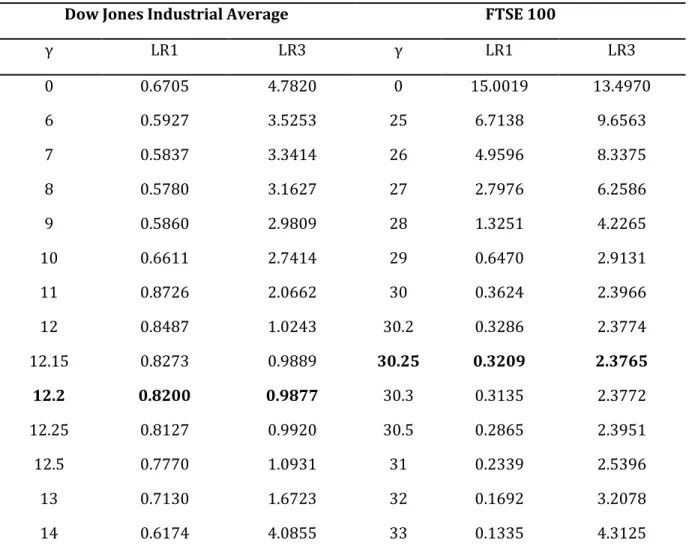
The following table exhibits the different values of and for different levels of risk aversion for the Dow Jones Industrial Average and the FTSE 100.

Dow Jones Industrial Average FTSE 100

γ LR1 LR3 γ LR1 LR3 0 0.6705 4.7820 0 15.0019 13.4970 6 0.5927 3.5253 25 6.7138 9.6563 7 0.5837 3.3414 26 4.9596 8.3375 8 0.5780 3.1627 27 2.7976 6.2586 9 0.5860 2.9809 28 1.3251 4.2265 10 0.6611 2.7414 29 0.6470 2.9131 11 0.8726 2.0662 30 0.3624 2.3966 12 0.8487 1.0243 30.2 0.3286 2.3774 12.15 0.8273 0.9889 30.25 0.3209 2.3765 12.2 0.8200 0.9877 30.3 0.3135 2.3772 12.25 0.8127 0.9920 30.5 0.2865 2.3951 12.5 0.7770 1.0931 31 0.2339 2.5396 13 0.7130 1.6723 32 0.1692 3.2078 14 0.6174 4.0855 33 0.1335 4.3125

Table 4 - Values of the likelihood ratios LR1 and LR3 for each value of the risk aversion estimate γ for both indexes. In bold are the optimum values of γ that minimise LR3.

(31)

27

With these likelihood ratios we can observe how accurately the densities are forecasting the future levels of prices. It is apparent that the real world densities that are the most accurate are those that were transformed with an assumed risk aversion of 12.2 and 30.25 for the Dow Jones Industrial Average and the FTSE 100 respectively. These values are superior to the 9.39 and 21.28 estimated with the method of maximum likelihood, however, they reinforce the idea that the optimal risk aversion values for the period under estimation are high and that the FTSE 100 displays an even higher risk aversion than the American index. Additionally, it can be observed that there is a marked improvement of the forecasting abilities of the transformed densities over the risk neutral density represented with a value of zero. Because the test statistic follows a chi-square distribution with three degrees of freedom, we can test if, for the optimal value of risk aversion, the variable is i.i.d. and follows a standard normal. We conclude that the p-values for the American and the English indexes are 0.804 and 0.498 respectively, which excludes the rejection of the null hypothesis for the most common levels of significance.

In all, even though the risk aversion comparison between the two indexes carried out in this analysis suggests that investors in the FTSE 100 have a higher aversion to risk than those investing in the Dow Jones Industrial Average, the results may prove inconclusive regardless of a wide difference between the two estimates of . As was seen, risk aversion is very sensitive to the volatility in the market and estimates prove to be unstable during short periods of analysis. A more definitive conclusion would be achieved by extending the period of study across several years in order to eliminate the effects of temporary peaks in volatility, as well as to average out the unexpected rises and drops of the markets that have a big influence on the values.

5 - Conclusions

The methods analysed in this study use option data to give valuable insight into the expectations of market participants as well as their risk preferences. Using three different methods to calculate the RND, we were able to conclude that, in this example, the mixture of lognormal distributions presents a good flexibility, the best fit to the observed information and was therefore chosen. For this method, the weights assigned to one of the lognormal distributions were low for both indexes, which leads to the conclusion that there is no expectation of a two-state economy. The existence of a second lognormal is then merely used to increase the density's flexibility concerning skewness and kurtosis, thus allowing it to display some of the empirically-found characteristics of equity price distributions. Although mostly satisfactory, the GB2 and the polynomial-lognormal methods have proved to be inferior when analysing the FTSE 100.

However interesting, the RND does not give information regarding the true expectations of investors or their risk aversion. To estimate these, we have assumed that investor's preferences are consistent with a power utility function with a constant relative risk aversion equal to the parameter . Using the method of maximum likelihood and a likelihood ratio introduced by Berkowitz (2001) resulted in different values of risk aversion for each index.

(32)

28

This apparent disparity can be explained by the relatively short number of periods considered in the analysis. Regardless of this shortcoming, both methods seem to support the fact that the risk aversion was high compared to that found in similar studies. In addition, they both suggest a higher risk aversion for the investors of the FTSE 100 index. Under the assumption that risk preferences are constant throughout long periods of time, it would be interesting to make the comparison of risk aversion between indexes using a longer time frame. The short time interval this study refers to may have impaired the conclusions drawn from the likelihood ratio test since it relies on a test of normality and independence. Also the method of maximum likelihood could benefit from a higher number of observed periods since we have witnessed a strong instability in the estimates across different observations. Analysing this instability, we have found evidence of the negative correlation between risk aversion and market volatility also supported in Bliss and Panigirtzoglou (2004). Furthermore, the maximum likelihood method relies on the assumption that the expectations of investors are, on average, an approximation of the true real world densities. Whenever there is a mistake in the expectations of investors in individual observations, this error is captured by the risk aversion estimate and can result in unlikely values.

(33)

29

Bibliography

Aït-Sahalia, Y. & Lo, A. W., 1998. Nonparametric Estimation of State-Price Densities Implicit in Financial Asset Prices. The Journal of Finance, 53(2), pp. 499-547.

Aït-Sahalia, Y. & Lo, A. W., 2000. Nonparametric risk management and implied risk aversion.

Journal of Econometrics, Issue 94, pp. 9-51.

Anagnou, I., Bedendo, M., Hodges, S. D. & Tompkins, R., 2005. Forecasting Accuracy of Implied and GARCH-Based Probability Density Functions. University of Warwick and HBF Frankfurt. Anagnou, I., Bedendo, M., Hodges, S. D. & Tompkins, R. G., 2002. The Relation Between Implied

and Realised Probability Density Functions, s.l.: Financial Options Research Centre, University

of Warwick.

Bahra, B., 1997. Implied Risk-neutral Probability Density Functions From Option Prices: Theory and Application. Bank of England Working Paper No 66 .

Bates, D. S., 1991. The Crash of '87: Was It Expected? The Evidence from Options Markets. The

Journal of Finance, 46(3), pp. 1009-1044.

Berkowitz, J., 2001. Testing Density Forecasts, With Applications to Risk Management. Journal

of Business & Economic Statistics, 19(4), pp. 465-474.

Black, F. & Scholes, M., 1973. The Pricing of Options and Corporate Liabilities. The Journal of

Political Economy, 81(3), pp. 637-654.

Bliss, R. R. & Panigirtzoglou, N., 2004. Option-Implied Risk Aversion Estimates. Journal of

Finance, Issue 59, pp. 407-446.

Bookstaber, R. M. & McDonald, J. B., 1987. A General Distribution for Describing Security Price Returns. The Journal of Business, 60(3), pp. 401-424.

Breeden, D. T. & Litzenberger, R. H., 1978. Prices of State-Contingent Claims Implicit in Option Prices. The Journal of Business, 51(4), pp. 621-651.

Buchen, P. W. & Kelly, M., 1996. The Maximum Entropy Distribution of an Asset Inferred from Option Prices. Journal of Financial and Quantitative Analysis, 31(1), pp. 143-159.

Bu, R. & Hadri, K., 2007. Estimating option implied risk-neutral densities using spline and hypergeometric functions. Econometrics Journal, Volume 10, pp. 216-244.

Campa, J. M., Chang, P. K. & Reider, R. L., 1998. Implied Exchange Rate Distributions: Evidence From OTC Option Markets. Journal of International Money and Finance, 17(1), pp. 117-160. Cochrane, J. H. & Hansen, L. P., 1992. Asset Pricing Explorations for Macroeconomics. NBER

(34)

30

Corrado, C. J. & Su, T., 1997. Implied Volatility Skews and Stock Index Skewness and Kurtosis Implied by S&P 500 Index Option Prices. The Journal of Derivatives, 4(4), pp. 8-19.

European Central Bank, 2011. THE INFORMATION CONTENT OF OPTION PRICES. ECB

Monthly Bulletin, February.

Fackler, P. L. & King, R. P., 1990. Calibration of Option-Based Probability Assessments in Agricultural Commodity Markets. American Journal of Agricultural Economics, 72(1), pp. 73-83.

Han, Y., 2002. On the Relation between the Market Risk Premium and Market Volatility. Jackwerth, J. C., 1999. Option-Implied Risk-Neutral Distributions and Implied Binomial Trees: A Literature Review. Journal of Derivatives, 7(2), pp. 66-82.

Jackwerth, J. C., 2004. Option-Implied Risk-Neutral Distributions and Risk Aversion. s.l.:The Research Foundation of AIMR™.

Jackwerth, J. C. & Rubinstein, M., 1996. Recovering Probability Distributions from Option Prices. The Journal of Finance, 51(5), pp. 1611-1631.

Jondeau, E. & Rockinger, M., 2000. Reading the smile: the message conveyed by methods which infer risk neutral densities. Journal of International Money and Finance, Issue 19, p. 885–915.

Liu, X., Shackleton, M. B., Taylor, S. J. & Xu, X., 2007. Closed-form transformations from risk-neutral to real-world distributions. Journal of Banking & Finance, Issue 31, pp. 1501-1520. Madan, D. & Milne, F., 1994. Contingent Claims Valued and Hedged by Pricing and Investing in a Basis. Mathematical Finance, 4(3), pp. 223-245.

Malz, A. M., 1997. Estimating the Probability Distribution of the Future Exchange Rate from Option Prices. The Journal of Derivatives, 5(2), pp. 18-36.

Mehra, R. & Prescott, E. C., 1985. The Equity Premium: A Puzzle. Journal of Monetary

Economics, Issue 15, pp. 145-161.

Ritchey, R. J., 1990. Call Option Valuation for Discrete Normal Mixtures. Journal of Financial

Research, 13(4), pp. 285-296.

Rosenberg, J. V. & Engle, R. F., 2002. Empirical pricing kernels. Journal of Financial Economics, Issue 64, pp. 341-372.

Shackleton, M. B., Taylor, S. J. & Yu, P., 2010. A multi-horizon comparison of density forecasts for the S&P 500 using index returns and option prices. Journal of Banking & Finance, Issue 34, pp. 2678-2693.

(35)

31

Taylor, S. J., 2005. Asset Price Dynamics, Volatility, and Prediction. s.l.:Princeton University Press.