Strategies for Optimize Off-Lattice Aggregate Simulations
S. G. Alves,∗ S. C. Ferreira Jr.,† and M. L. Martins‡
Departamento de F´ısica, Universidade Federal de Vic¸osa, 36570-000, Vic¸osa, MG, Brazil
Received on, 27 September, 2007
We review some computer algorithms for the simulation of off-lattice clusters grown from a seed, with empha-sis on the diffusion-limited aggregation, ballistic aggregation and Eden models. Only those methods which can be immediately extended to distinct off-lattice aggregation processes are discussed. The computer efficiencies of the distinct algorithms are compared.
Keywords: Off-lattice aggregation; Diffusion-limited aggregation; Ballistic aggregation; Eden model
I. INTRODUCTION
Growth processes occurring far from equilibrium are wide-spread in nature and technology. Examples include electrode-position [1], viscous fingering [2], bacterial colonies [3], and neurite formation [4]. Computer models for the growth of clusters, generally constituted of identical particles, are use-ful tools for the understanding of aggregation phenomena. The main contribution of such models is to provide pathways to investigate the underlying physical ingredients ruling the properties observed in growth phenomena. One of the most intriguing features of the fractal structures found in nature and computer models is the scale invariance emerging with-out fine-tuning of any parameter, in contrast with usual crit-ical phenomena in which scale invariance only emerges at a critical point [5].
The foremost example of nonequilibrim growth model is the diffusion-limited aggregation (DLA) model introduced by Witten and Sander [6] in 1981. The rules of the DLA model are based on an iterative stochastic process in which the par-ticles, one at a time, follow Brownian trajectories until they touch and stick in an aggregate. Despite its simple rules, the DLA model leads to very complex aggregates with multiscale properties [7, 8] and multifractality in the growth-site proba-bility distribution [9, 10].
If the random walks in the DLA model are replaced by bal-listic trajectories at random directions, we have the balbal-listic aggregation (BA) model [11, 12] proposed by Vold to describe colloid aggregation. Differently from DLA, the BA model generates asymptotically non-fractal clusters (fractal dimen-sion equal to the space dimendimen-sion) characterized by a power law approach to the asymptotic regime [13, 14].
Finally, a third standard aggregation process was proposed by Eden [15] as a basic model for the biological pattern forma-tion as, for instance, tumor growth and bacterial colonies. In this model, new particles are sequentially added to the empty neighborhood of the cluster without overlap with previously aggregated particles [16, 17]. Although the Eden model is unrealistic from the biological point of view, it produces
com-∗Electronic address:[email protected]
†Electronic address:[email protected] ; (Corresponding Author.) ‡Electronic address:[email protected]
pact aggregates with a nontrivial interface scaling usually ana-lyzed through the interface widthw[18]. Intensive numerical simulations indicate a power-law growth of the interface width with the time,w∼tβ, and exponentβ=1/3 [14, 17, 19, 20], corresponding to the Kardar-Parisi-Zhang (KPZ) universality class [21].
The DLA, BA, and Eden models can be implemented and simulated in a relatively easy way by constraining the particle positions to the sites of an underlying lattice. However, it is very well established that lattice anisotropy imposes strong ef-fects on the cluster shape and scaling [22–25]. Although some procedures have been proposed to remove the anisotropy of on-lattice clusters [26–28], their successes were limited and off-lattice simulations impose themselves as a general frame-work for the investigation of the scaling properties and uni-versality classes of these aggregates. Clearly, the aggregation of a large number of particles is necessary to reach the as-ymptotic behavior which, in turn, demands very efficient al-gorithms for large scale off-lattice simulations with rigorous statistical sampling. In this paper, we review several strate-gies used to optimize computer algorithms for off-lattice ag-gregates. Only those procedures which can be applied to gen-eral off-lattice simulations are focused here. More sophisti-cated but less general procedures, as conformal maps [29], are avoided. Indeed, the conformal mapping is the most efficient strategy to simulate two-dimensional aggregates, but it cannot be used in higher dimensions.
II. ALGORITHMS FOR OFF-LATTICE AGGREGATION
In this section we present the description of distinct opti-mizations for two-dimensional clusters. The generalization for higher dimensions is straightforward. In all cases, simula-tions start with a single particle at the origin.
A. The trajectories
[a]
r
max
r
k
r
l
r
ext
r
int
[b] [c]
2r
int
r
int
r
int
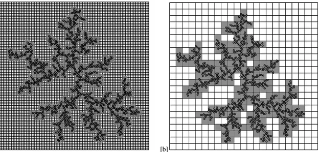
FIG. 1: (a) Schematic representation of the “optimized random trajectories”. (b) A DLA aggregate and a mesh of cells 2rint×2rint. Long steps are forbidden in the gray boxes and allowed in the white ones. Also, two long steps are illustrated. (c) A zoom of the region inside the large square in (b).
rkmuch larger than the system size. In the DLA, where
par-ticles follow discrete time random walks of unitary steps, a standard method is to allow the particles outside the launching circle take long random steps of lengthrextif these steps do not
brings up a particle inside the launching circle, as illustrated in Fig. 1(a). An adequate choice isrext=max(r−rmax−δ,1),
where ris the distance of the walker from the origin and a small toleranceδ=5 was used. Also, the Brownian walks in large empty areas in the inner region which delimits the clus-ter (r<rmax) are very computer time consuming, specially
for large aggregates. Ball and Brady [30] proposed a strategy which allows the particles inside the launching circle to take a long step of lengthrint if they do not cross any part of the
aggregate, as illustrated in Fig. 1(a). Similar procedures have been used in other works [31–33].
In the BA model, the particles follow ballistic trajectories and the clusters do not exhibit large empty inner regions as in the DLA model. Hence, the trajectories can be efficiently implemented simply using a long step of sizerext as in DLA
model. An important difference between BA and DLA imple-mentations is that in the first the launching radius should be as large as possible in order to avoid growth instabilities pro-moted by shadowing effects [34, 35] while in the DLA, this radius can be taken a few particle diameters larger than the cluster radius.
A smart strategy to determine the length of the internal steps rint is decisive for the algorithm efficiency. In order to
accomplish this task, we define a square region of sideL cen-tered on the initial seed which delimits the entire aggregate. This region should be sufficiently large in order to guaran-tee that aggregate does not exceed its boundary. Then, the region is divided in a coarse-grained mesh with cells of size 2rint×2rint as illustrated in Figs. 1(b) and 1(c). Each cell of
the mesh is associated to an element of aK×Ksquare matrix
A
, whereK=L/(2rint), which assumes 1 if the cell or one ofits nearest or next-nearest neighbors contains any particle of the aggregate or assumes 0 otherwise. The boxes depicted in gray (
A
i j=1) are those in which the random walk can cross the cluster after a step of lengthrint, since they contain or areadjacent to a part of the cluster. Consequently, long steps
start-ing from gray boxes are forbidden. There are two options for a walker on a gray box: the particle executes a unitary step or tries a shorter step of lengthr′
int, where 1<r′int<rint,
us-ing other auxiliary coarse-grained mesh
A
′with cells of size 2r′int×2r′int. Indeed, several auxiliary meshes can be used in
order to maximize the efficiency. In this paper, we report sim-ulation for 3 meshes withrint=4,8,and 16.
The overlap between particles can occur after a unitary step if the preceding step brings the random walker at a distance from the cluster particle where it sticks lower than the unity. In this case, one just brings back the particle to the adjacent position along the opposite direction of the movement.
B. Determination of the neighborhood
re-[a] [b]
FIG. 2: Illustration of the optimizations for off-lattice aggregation processes. (a) An auxiliary square lattice is used to determine when the walker is neighboring the cluster. The cluster particles are represented by black circles and their neighbors are depicted in gray. (b) A mesh with cells of size 4×4 used to restrict the search for contacts nearby the walker.
[a]
1
2
[b] [c]
FIG. 3: Growth rules for the off-lattice Eden model. Active and inactive particles are represented by open and fullfiled discs, respectively. (a) A cluster and two active particles selected for the growth. The particle 1 has an empty region where a new adjacent particle can be added while the particle 2 does not. (b) The growth region adjacent to the particle 1 is shown as a dashed sector. (c) A new particle is added at a random direction in the growth region shown in (b) and the particle 2 is discarded from the list of active ones (both indicated by arrows).
gion around the walker position. In this strategy, the cells are sequentially labeled by an indexk=1,2,3,· · ·when they are occupied by a particle of the cluster for the first time. Also, the number of particlesNkin the cells are stored. Finally, a third
auxiliary one-dimensional array
F
divided in blocks withℓ2elements is used to store the indexes of the particles in the ar-rays of coordinates. Each block is associated to a cell of the mesh. Once the analysis of the auxiliary square matrix
Z
has provided that the walker may be in contact with a particle of the cluster, the indexkread in the meshW
is used to restrict the search for a contact in the array of coordinates usingF
. The cell index of a walker at real coordinates(x,y)is given by k=W
i j, wherei=nint(x/ℓ),j=nint(y/ℓ), and nint(x) func-tion roundsxto the nearest integer. Indeed, the particles in the cellkare visited by varying the index of the arrayF
from n=nk+1 ton=nk+Nk, wherenk=ℓ2×(k−1). Notice thatthe cell jof the mesh
W
and its neighbor cells should bever-ified to check the contacts on the cell edges. In the simulation results presented in the next section,ℓ=4 was used.
C. The Eden model
The off-lattice simulation of the Eden model was proposed by Wang et al. [16] and improved by Ferreira and Alves [17] as follows
• A particle with unitary diameter is chosen at random from a list of active ones (Fig. 3(a)). A particle is con-sidered active when a new one adjacent to it can be added to the aggregate without any overlap.
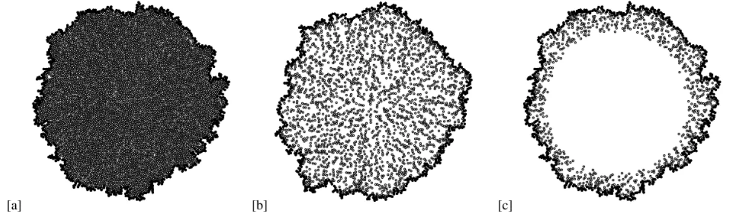
[a] [b] [c]
FIG. 4: (a) Eden cluster with 6000 particles. The border is represented by fullfiled symbols. Active particles for (b) standard and (c) optimized off-lattice algorithms for the Eden model are shown.
103 104 105 106
N
10-3 10-2 10-1 100 101 102 103 104 105
CPU Time (min) O
0
O
1
O
2
O
3
FIG. 5: CPU times as functions of the number of particles in the off-lattice DLA model for distinct optimization strategies. Lines are power fits.
new particle and those previously aggregated, is deter-mined. A new particle is put in a direction randomly chosen among the allowed ones (Fig.3(b)).
• If the active particle does not have a growth region, it is
labeled as inactive (Fig.3(c)).
In Fig, 3 the evolution rules are illustrated by two indepen-dent growth processes. Since the interest on Eden clusters is focused on the interface scaling, Ferreira and Alves [17] intro-duced an optimization where any active cell inside a central core of radius rc is labeled as inactive. Since the inactiva-tion of the particles near or belonging to the interface must be avoided,rc=0.8¯rwas chosen, where ¯ris the mean radius of the interface. This optimization was used only for ¯r>80a. In Fig. 4, typical growth patterns with and without this last optimization, the corresponding borders [36], and the active particles are illustrated. Finally, the optimizations described in sub-section II B for determining the neighborhood of a par-ticle can be used for the Eden model.
III. SIMULATIONS
All simulations were performed on the same computer, a Pentium IV 3.0 GHz with 2GB of RAM memory under De-bian Linux operating system. One process was run by time. The algorithm codes were written in FORTRAN 90 language and compiled with the standard options of the Intel Fortran Compiler 9.1 [37].
A. Diffusion-limited aggregation
Off-lattice DLA clusters withN particles were grown us-ing different combinations of the previously described opti-mizations. In all simulations, the launching and killing radius were taken asrl =rmax+5 andrk=100rl, respectively. In 1981, when Sander and Witten published their seminal work introducing the DLA model [6] without any optimization, the largest cluster generated on square lattices produced with computers of that age did not reach 4000 particles. Nowadays, this sort of simulation can be performed in a few minutes with any standard home computer. In table I, the CPU times spent in off-lattice simulations of a single cluster for some optimiza-tion schedules are listed. Also, CPU times are shown as func-tions ofNin Fig. 5.
N O0 O1 O2 O3 1×10³ 3.93
×100 1.62×10⁻³ 1.6×10⁻³ 1.6×10⁻³
2×10³ 1.38×101 5.81×10⁻² 1.3
×10−2 8.3
×10−3
5×10³ 8.79×101 6.37×100 3.0×10⁻² 2.5
×10−2
1×10⁴ 3.48×10² 4.29×101 8.8×10⁻² 4.0
×10−2
2×10⁴ 2.57×10³ 2.49×10² 3.7×10⁻¹ 8.8
×10−2
5×10⁴ 1.37×10⁴ 2.69×10³ 2.25×100 2.3×10⁻¹ 1×10⁵ — 2.94×10⁴ 8.33×100 5.0×10⁻¹
2×10⁵ — — 1.74×101 1.55×100
5×10⁵ — — 1.76×10² 6.60×100
1×10⁶ — — 8.73×10² 2.60×101
CPU time T∼N2.1 T ∼N2.8 T∼N1.9 T∼N1.4
TABLE I: Real CPU times in minutes for distinct optimizations ap-plied to the DLA model. N is the number of particles; O0 refers to the algorithm with the default optimization where the backward inspetion of the coordinate arrays is used;O1means that the long ex-ternal steps of sizerextwere used;O2means that external steps and optimized neighborhood were used simultaneously;O3the previous optimizations plus the internal long steps of sizerint(Figs. 1 and 2) were adopted. The approximate dependence between CPU time and cluster size are indicated in the last line.
103 104 105 106 107
N
10-3 10-2 10-1 100 101 102 103 104
CPU Time (min) O
0
O
1
O
2
O
3
FIG. 6: CPU times as functions of the number of particles in the off-lattice BA model for distinct optimization strategies. Lines are power fits.
Also, notice that the computational time increases faster in O1than in the others optimizations, but for large clustersO0 andO1optimizations are expected to be equivalent due to the presence of large empty inner regions.
B. Ballistic aggregation
Off-lattice simulations of the BA model are very similar to the DLA model. The main difference is that the unitary steps performed by the walkers are in a fixed direction randomly chosen at the beginning of the ballistic walk. Also, the launch-ing and killlaunch-ing radius used were rl =100rmax+1000 and rk=rl+10. In table II, the computational times for the same
104 105 106 107
N
10-1 100 101 102 103
CPU Time (min)
E
0
E
1
E
2
FIG. 7: CPU times as functions of the number of particles in the off-lattice Eden model using distinct optimization strategies. Lines are power fits.
N O0 O1 O2
1×10³ 2.81×10⁻¹ 1.51
×10−2 1.35
×10−2
2×10³ 6.45×10⁻¹ 2.78
×10−2 2.09
×10−2
5×10³ 1.96×100 1.08×10⁻¹ 2.27
×10−2
1×10⁴ 4.78×100 4.63×10⁻¹ 3.62
×10−2
2×10⁴ 1.29×101 2.03×100 6.10×10⁻² 5×10⁴ 5.44×101 1.43×101 1.34×10⁻¹ 1×10⁵ 1.67
×102 5.99×101 2.52×10⁻¹
2×10⁵ 6.10×10² 2.85×10² 4.94×10⁻¹ 5×10⁵ 3.50×10³ 2.18×10³ 1.22×100
1×10⁶ — — 2.43×100
2×10⁶ — — 5.01×100
5×10⁶ — — 1.29×101
5×10⁶ — — 2.61×101
TABLE II: Real CPU time in minutes for distinct optimizations ap-plied to BA model. Optimizations as in table I.
strategies used for DLA are listed. Like in the DLA model, long steps improve simulation efficiency for small clusters, but this gain decreases with increasing number of particles. However, optimized neighborhood determination provodes a gain of three orders of magnitude. In Fig. 6 the CPU times are drawn as functions ofN. These times grow approximately as T∼N1.7,T∼N2.1, andT ∼N1.0forO0,O1, andO2, respec-tively.
C. Eden model
N E0 E1 E2 1×10³ 1.12×10⁻² 1.33
×10−2 1.33
×10−2
2×10³ 2.04
×10−2 1.33×10⁻² 1.33×10⁻²
5×10³ 7.31×10⁻² 1.60
×10−2 1.83
×10−2
1×10⁴ 3.63×10⁻¹ 2.33
×10−2 2.33
×10−2
2×10⁴ 1.92×100 3.67×10⁻² 3.33
×10−2
5×10⁴ 1.92×101 8.33×10⁻² 6.00
×10−2
1×10⁵ 1.09×10² 1.81×10⁻¹ 1.20×10⁻¹ 2×10⁵ 6.13×10² 4.72×10⁻¹ 2.40
×10−1
5×10⁵ — 1.70
×100 7.30×10⁻¹
1×10⁶ — 4.63×100 1.78×100 2×10⁶ — 1.26×101 4.55×100 5×10⁶ — 4.89×101 1.62×101
TABLE III: Eden Model Optimizations. SymbolsE0, E1, and E2 described in text.
the model is denoted byE1. CPU times are given in table III and Fig. 7. The last algorithm overcomes the first one in three or more orders of magnitude. If a central core of particles is excluded from the list of active ones, the optimizationE2, simulations become up to three times faster. Moreover, the
efficiency gain increases with the number of particles. Indeed, CPU times grow approximately asT ∼N2.5,T ∼N1.4, and T∼N1.2forE0,E1, andE2, respectively.
IV. SUMMARY
Several optimizing strategies for the computer simulation of aggregation models dispersed throughout the literature were described in the present paper. It have been demon-strated that the combined implementation of such strategies can reduce in up to four order of magnitude the computer time demanded to perform large scale simulations of off-lattice ag-gregates with an increase of one order of magnitude in the allocated memory. Furthermore, these procedures can be ap-plied to the simulations of other cluster growth processes be-yond the traditional DLA, BA, and Eden models.
Acknowledgments
This work was partially supported by CNPq and FAPEMIG, Brazilian agencies. We thank to Nem´esio M. Oliveira-Neto for non expertise reading of the manuscript and his valuable contribution to make the paper more accessible.
[1] M. Matsushita, M. Sano, Y. Hayakawa, H. Honjo, and Y. Sawada, Phys. Rev. Lett.53, 286 (1984).
[2] K. J. M˚aløy, J. Feder, and T. Jøssang, Phys. Rev. Lett.55, 2688 (1985).
[3] M. Matsushita and H. Fujikawa, Physica A168, 498 (1990). [4] F. Caserta, H. E. Stanley, W. D. Eldred, G. Daccord, R. E.
Haus-man, and J. Nittmann, Phys. Rev. Lett.64, 95 (1990).
[5] H. E. Stanley, Introduction to phase transitions and Critical Phenomena(Oxford University Press, Cambridge, 1971). [6] T. A. Witten and L. M. Sander, Phys. Rev. Lett.47, 1400 (1981). [7] C. Amitrano, A. Coniglio, P. Meakin and M. Zanneti, Phys.
Rev. B44, 4974 (1991).
[8] B. B. Mandelbrot, B. Kol, and A. Aharony, Phys. Rev. Lett.88, 055501 (2002).
[9] C. Amitrano, A. Coniglio, and F. Diliberto, Phys. Rev. Lett.57, 1016 (1986).
[10] L. M. Sander, Contemp. Phys.41, 203 (2000). [11] M. J. Vold, J. Colloid. Sci.18, 684 (1963).
[12] P. Meakin,Fractals, scaling and growth far from equilibrium (Cambridge University Press, Cambridge, 1998).
[13] S. Liang and L. P. Kadanoff, Phys. Rev. A31, 2628 (1985). [14] T. Vicsek,Fractal Growth Phenomena(World Scientific,
Sin-gapore, 1992).
[15] M. Eden, in J. Neyman (ed.), Proceedings of the 4th Berke-ley Symposium on Mathematical Statistics and Probability Vol. 4: Biology and Problems of Health, (University of California Press) (1961).
[16] C. Y. Wang, P. L. Liu, and J. G. Bassingthwaighte, J. Phys. A: Math. Gen.28, 2141 (1995).
[17] S. C. Ferreira Jr. and S. G. Alves, J. Stat. Mech.: theory and experiment P11007 (2006).
[18] The interface width is commonly defined as the standard devi-ation of the distances from the center of the lattice.
[19] J. Kert´esz and D. E. Wolf, J. Phys. A: Math. Gen. 21, 747 (1988).
[20] P. Devillard and H. E. Stanley, Physica A160, 298 (1989). [21] M. Kardar, G. Parisi and Y. C. Zhang, Phys. Rev. Lett.56, 889
(1986).
[22] S. Tolman and P. Meakin, Phys. Rev. A40, 428 (1989) [23] N. R. Goold, E. Somfai, R. C. Ball, Phys. Rev. E72, 031403
(2005).
[24] J. G. Zabolitzky and D. Stauffer, Phys. Rev. A34, 1523 (1986). [25] M. J. Batchelor and B. I. Henry, Phys. Lett. A157, 229 (1991). [26] L. R. Paiva and S. C. Ferreira, J. Phys. A. Math. Gen.40, F43
(2007).
[27] S. G. Alves and S. C. Ferreira, J. Phys. A. Math. Gen.39, 2843 (2006).
[28] V. A. Bogoyavlenskiy, J. Phys. A. Math. Gen.35, 2533 (2002). [29] B. Davidovitch, H. G. E Hentschel, Z. Olami1, I. Procaccia1,
L. M. Sander, and E. Somfai, Phys. Rev E.59, 1368 (1999). [30] R. C. Ball and R. M Brady, J. Phys. A: Math. Gen.18, L809
(1985).
[31] P. Meakin and T. Vicsek, Phys. Rev. A32, 685 (1986). [32] S. G. Alves and S. C. Ferreira, Phys. Rev. E73, 051401 (2006). [33] S. C. Ferreira, Eur. Phys. J. B42, 263 (2004).
[34] C. Tang and S. Liang, Phys. Rev. Lett.71, 2769 (1993). [35] J. Yu and J. G. Amar, Phys. Rev. E66, 021603 (2002). [36] The border is defined as the set of cells that forms an external
layer impenetrable for incoming cells. Consequently, the spaces between consecutive border cells is smaller than a cell diameter. [37] The free non-commercial version of the Intel Fotran Compiler
for linux was take from http://www.intel.com/cd/ software/products/asmo-na/eng/compilers/