Influence of snow depth distribution on surface roughness in alpine terrain: a multi-scale approach

(1)

terrain: a multi-scale approach

J. Veitinger1, B. Sovilla1, and R. S. Purves2

1_{WSL Institute for Snow and Avalanche Research SLF, Davos, Switzerland} 2_{Department of Geography, University of Zurich, Zurich, Switzerland} Correspondence to:J. Veitinger ([email protected])

Received: 16 July 2013 – Published in The Cryosphere Discuss.: 13 September 2013 Revised: 17 January 2014 – Accepted: 18 February 2014 – Published: 3 April 2014

Abstract.In alpine terrain, the snow-covered winter surface deviates from its underlying summer terrain due to the pro-gressive smoothing caused by snow accumulation. Terrain smoothing is believed to be an important factor in avalanche formation and avalanche dynamics, and it affects surface heat transfer, energy balance as well as snow depth distri-bution. To assess the effect of snow on terrain, we use an adequate roughness definition. We developed a method to quantify terrain smoothing by combining roughness calcu-lations of snow surfaces and their corresponding underly-ing terrain with snow depth measurements. To this end, el-evation models of winter and summer terrain in three se-lected alpine basins in the Swiss Alps characterized by low, medium and high terrain roughness were derived from high-resolution measurements performed by airborne and terres-trial lidar. The preliminary results in the selected basins re-veal that, at basin scale, terrain smoothing depends not only on mean snow depth in the basin but also on its variabil-ity. The multi-temporal analysis over three winter seasons in one basin suggests that terrain smoothing can be modelled as a function of mean snow depth and its standard deviation using a power law. However, a relationship between terrain smoothing and snow depth was not found at pixel scale. Fur-ther, we show that snow surface roughness is to some extent persistent, even in-between winter seasons. Those persistent patterns might be very useful to improve the representation of a winter terrain without modelling of the snow cover distri-bution. This can for example improve avalanche release area definition and, in the long term, natural hazard management strategies.

1 Introduction

During and after a snowfall event, wind, snow gliding and avalanches redistribute snow and smooth the geomorphol-ogy of the terrain by filling irregularities. During the snow accumulation season, terrain features successively disappear, leading to increasingly homogeneous deposition patterns during storm events and, thus, to a progressive smoothing of the terrain surface. Terrain smoothing influences albedo (e.g. Manninen et al., 2012), surface heat transfer and en-ergy balance (e.g Fassnacht et al., 2009) and/or snow depth distribution (Mott et al., 2010). Whereas albedo is mainly affected by millimetre to centimetre changes of the winter terrain surface, snow distribution processes are modified by a changing winter topography at scales up to several tens of metres. Thus, understanding the multi-scale effects of snow smoothing on topography is very important in avalanche haz-ard assessment, run-off modelling and water resource man-agement.

(2)

explain the observed differences in release areas.

The importance of snow cover distribution in avalanche formation processes is well known and widely mentioned in the literature. One parameter particularly highlighted in this context is roughness. For a shallow snowpack, roughness can have a stabilizing function hindering the formation of contin-uous weak layers (Schweizer et al., 2003) and slabs (Simen-hois and Birkeland, 2008) as well as providing mechanical support to the snowpack. McClung (2001) showed in a study of 76 avalanche paths due to clear-cut logging in the Coast and Columbia mountains of British Columbia that ground roughness (defined in a categorical way: (1) low: ground fea-tures smaller than 1 m relief; (2) medium: ground feafea-tures 1–2 m relief; (3) high: ground features bigger than 2 m re-lief) is potentially important in inhibiting avalanche initia-tion. Actually, no events were reported in areas with rough-ness height larger than 2 m. Moreover, van Herwijnen and Heierli (2009) stated that, in the case of weak layer failure, roughness of the bed surface plays an important role in de-termining whether an avalanche will release or not. However these stabilizing effects of terrain roughness disappear if the snowpack is deep enough to form a relatively smooth inter-mediate surface (McClung and Schaerer, 2002) where the formation of a homogenous snowpack with continuous weak layers and slabs is facilitated. All these studies demonstrate the ability of roughness to capture terrain smoothing as well as its importance in avalanche formation processes.

In recent years, airborne (Vallet, 2011; Fischer et al., 2011) and terrestrial laser scanning (Grünewald et al., 2010; Prokop, 2008; Prokop et al., 2008) have become increasingly reliable and feasible techniques to obtain high-resolution snow depth measurements even in steep alpine terrain, allow-ing analysis of snow depth distribution over multiple scales (Schirmer and Lehning, 2011; Deems et al., 2008; Trujillo et al., 2007). The importance of scale in snow redistribu-tion is widely recognized. For instance it is known that snow redistribution patterns vary over scales due to different un-derlying processes (Blöschl, 1999). Winstral et al. (2002) suggested that one reason for the low percentage of snow depth variation that can be explained by terrain parameters might be differences in modelled processes and scales. Ac-cordingly, methods like fractal analysis have been applied to evaluate snow depth variability over a wide range of scales (Schirmer and Lehning, 2011; Deems et al., 2008, 2006).

et al. (2011) established a statistical relationship between to-pography and snow depth in small topographical units. While Grünewald et al. (2013) showed that this behaviour is not universal, they stressed again the consistency of such sta-tistical models at a given field site for consecutive years at times of maximum snow accumulation. Although these stud-ies have brought valuable insight into snow depth distribution and its persistent topographical control in alpine terrain, little focus was put on how snow depth affects roughness of a win-ter win-terrain surface. Schirmer and Lehning (2011) inwin-terpreted the two distinct fractal scaling behaviours of snow depth in combination with increasing scale breaks in the accumula-tion season as smoothing of terrain roughness at increasing scales. Schweizer et al. (2003) stated that a snow depth of 0.3 to 1 m is required to eliminate terrain roughness. However, a consistent method to quantify the influence of snow depth on the geomorphology of a terrain surface integrating scale dependency and the temporal consistency of these processes has not been attempted yet.

In this study we provide a method to characterize and quantify the smoothing effects of snow on terrain based on high-resolution, multitemporal lidar measurements of sum-mer and winter terrain. To this end, we derive local rough-ness estimates based on gemorphological parameters of win-ter and summer win-terrain. First, we develop a method to capture and quantify terrain smoothing at basin as well as at pixel scale as a function of snow depth parameters. We apply and discuss the method, using lidar data of three geomorphologi-cally different basins within two alpine field sites in the Swiss Alps. Finally, we assess and quantify the persistence of snow depth and its corresponding terrain smoothing effects.

2 Methods and data

2.1 Field sites and data acquisition

(3)

2600 m a.s.l., and the orientation ranges from NE through E to SE. Steep slopes are located near the ridge, flattening out in the lower part of the basin. The terrain surface is less rugged and irregular than in CB1 but still contains more to-pographical variety, such as gullies and rocky outcrops, than CB2. The mean slope of the basin is 35.6◦_{with a standard} de-viation of 7.3◦_{. Slope maps of all basins are shown in Fig. 2.} Further, all three basins represent areas where avalanches can potentially release (slope angle steeper than 28◦).

Snow distribution in the Steintälli basin was determined by terrestrial laser scanning (TLS). The Riegl LPM-321 de-vice, operating at 905 nm, was used. This device has proven its ability to work in harsh alpine environment with sufficient accuracy (Prokop, 2008; Prokop et al., 2008). Grünewald et al. (2010) compared TLS with tachymeter measurements and found a mean deviation of 4 cm with a standard devia-tion of 5 cm at distances up to 250 m. Our measurement dis-tances ranged from 200 up to 600 m; thus we estimate our vertical measurement accuracy of 20 cm or better. To ensure scan quality, we further performed reproducibility tests. We always performed a scan in coarse resolution in the begin-ning of the measurement campaign in addition to the normal laser scan acquisition. This allowed us in the post-processing to detect misalignments between the two, indicating possi-ble errors due to an unstapossi-ble scanner setup (stability of tri-pod, wind influence, etc.). Only scans with a mean deviation of less than 10 cm of the coarse scan were considered. We produced raster maps with a spatial resolution of 1 m. We performed in total eight scans of the winter terrain between January and March within the winter seasons of 2010/11, 2011/12 and 2012/13. An additional scan of the summer ter-rain was acquired on 18 September 2011 and serves as a ref-erence for the snow depth calculations.

At the Vallée de la Sionne site, airborne laser scan-ning (ALS) measurements are performed before and after avalanche events using a helicopter-based system, and a de-tailed description of the method and the precision of the mea-surements can be found in Sovilla et al. (2010). The vertical accuracy of the data is 0.10 m. We resampled the original grid from 0.5 m resolution to 1 m resolution using cubic interpo-lation to have the same spatial resolution as in Steintälli. At the Vallée de la Sionne test site, three ALS measurements were performed in three different winter seasons.

To calculate snow depth, the summer terrain was sub-tracted from the winter terrain and negative snow depth

val-The ST field site serves as an example for the exploitation of mulitemporal acquisitions over a larger time span (eight scans over three winter seasons). The comparison with the VdlS field site, where only three data sets are available, is intended to illustrate the differences with respect to different terrain morphology.

2.2 Surface roughness calculation

In general we understand as roughness the variability of a to-pographical surface at a given scale. A number of definitions of roughness exist; for a recent overview see Grohmann et al. (2011). We decided to choose the vector ruggedness measure developed by Sappington et al. (2007) and based on the vec-tor approach proposed by Hobson (1972). In a preliminary step, the elevation gradient in both thexandy directions of a grid cell and its eight neighbouring cells is used to calcu-late the magnitude (slope),α, and the direction (aspect),β, of steepest gradient (Horn, 1981). We definea,bandcas the upper left, upper central and upper right pixel respectively;d

andf as the central left and central right pixel respectively; andg,handias the lower left, lower central and lower right pixel respectively (Fig. 3). We denote

dz

dx =

(c+2f+i)−(a+2d+g) (8·cellsizex)

, (2)

dz

dy =

(g+2h+i)−(a+2b+c) (8·cellsizey)

, (3)

wherea...irepresent the elevation of the corresponding cells and cellsizexand cellsizeycorrespond to the size of the grid

cell inx andy direction, respectively. Slope and aspect are then calculated using the following formulas:

α=arctan



sdz

dx 2 + dz dy 2

, (4)

β=arctan dz dy dz dx ! . (5)

(4)

CB2

CB1

ST

Fig. 1.Field sites Vallée de la Sionne (left) and Steintälli (right). In red are marked the exact location of the analysed basins CB1, CB2 and ST, and in green the location of the weather stations. Pixmaps©2013 swisstopo (5704 000 000).

−1. Consequently, trigonometric operations using these val-ues are treated as 0. Based on these definitions, normal unit vectors of every grid cell of a digital elevation model (DEM) are decomposed intox,yandzcomponents (Fig. 4, Eqs. 6– 9):

z=1·cos(α), (6)

xy=1·sin(α), (7)

x=xy·cos(β), (8)

y=xy·sin(β). (9)

A resultant vector|r|is then obtained for every pixel by sum-ming up the single components of the centre pixel and its neighbours using a moving window technique. The neigh-bourhood size can be set by the user and is defined by the number of pixelsntaken into account.

|r| =

q

(Xx)2₊₍X_y)2₊₍X_z)2_, ₍₁₀₎

as shown in Fig. 4b. The magnitude of the resultant vector is then normalized by the number of grid cellsnand subtracted from 1:

R=1−|r|

n, (11)

whereRis the vector ruggedness measure.

The result is a measure of the surface roughness with val-ues ranging from 0 (flat) to 1 (extremely rough). This defi-nition makes it possible to derive roughness directly from a DEM, and the moving window technique allows us to cal-culate local, pixel-based estimates of roughness. Since the method incorporates both the aspect and slope of the ele-vation gradient, we can distinguish between constant slope with constant aspect and constant slope with changing as-pect (Fig. 4c). Sappington et al. (2007) showed that the vec-tor ruggedness measure is uncorrelated with slope. The mea-sure has already been applied in different research fields, in-cluding, among others, animal habitat analysis (Sappington et al., 2007), avalanche dynamics (Sovilla et al., 2012) and avalanche formation (Vontobel, 2011).

(5)

2.3 Terrain smoothing assessment

Snow changes the underlying terrain by filling gullies and covering rocks; it also creates drift features such as dunes and cornices, which may be uncorrelated with the underly-ing terrain. Thus, to evaluate terrain smoothunderly-ing it is necessary to both calculate the degree of attenuation of terrain features produced by snow and estimate the degree of similarity be-tween winter and summer surface. In this study, we use the roughness calculations to assess the terrain smoothing pro-cesses.

To quantify terrain smoothing at basin scale, we performed a linear regression analysis between all pixels of a winter and

Fig. 3.Calculation of the horizontal and vertical gradient at grid celle, using the elevation values of the centre celleand its eight neighbours. Gradients are calculated for each grid cell in the input raster using a 3×3 window.

the corresponding summer surface of the form

RS=b×RT, (12)

wherebis the slope of the regression fit. We then denote the smoothing factorF:

F =1−b. (13)

F ranges between 0, when surface roughness is equal to ter-rain roughness and no smoothing is observed, and 1 for a complete even snow surface. Theoretically,F can be neg-ative for snow surfaces which are rougher than the terrain surface.

Further, we calculate the coefficient of determination,R2, of the regression fit, which determines the degree of similar-ity between the snow surface and terrain surface. High val-ues, up to 1, indicate that the underlying terrain is still domi-nating and the influence of snow is low. Low values indicate that snow influence is dominant, creating significant changes of the surface structure. Thus, these measures,F andR2 de-fine terrain smoothing at basin scale.

At pixel scale, terrain smoothing is analysed as a function of the roughness of the summer terrain as well as of the snow depth at this position. We assume that terrain smoothing is dependent on the value of the terrain roughness under con-sideration. We binned terrain roughness values into classes separated by intervals of 0.002. For each class with similar terrain roughness, snow surface roughness is analysed as a function of snow depth.

To quantify intra- and interannual persistence of snow depth and surface roughness, we calculate the degree of cor-relation between two distinct winter snow covers using the coefficient of determination,R2.

3 Results and discussion

3.1 Snow depth distribution

(6)

Fig. 4.Calculation of vector ruggedness measureR.(a)Decomposition of normal unit vectors of a DTM grid cell intox,yandzcomponents using slopeαand aspectβ.(b)Resultant vectorris obtained by summing up thex,yandzcomponents of all pixelsnwithin the neigh-bourhood window.(c)Vector ruggedness measure in flat (left), steep and even (middle), as well as steep and uneven terrain (right). Graphics from Sappington et al. (2007).

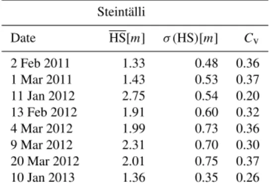
Table 1. Mean HS, standard deviationσ (HS) and coefficient of variationCvof snow depth distribution for every laser scan

acqui-sition in the ST basin.

Steintälli

Date HS[m] σ (HS)[m] Cv

2 Feb 2011 1.33 0.48 0.36

1 Mar 2011 1.43 0.53 0.37

11 Jan 2012 2.75 0.54 0.20

13 Feb 2012 1.91 0.60 0.32

4 Mar 2012 1.99 0.73 0.36

9 Mar 2012 2.31 0.70 0.30

20 Mar 2012 2.01 0.75 0.37

10 Jan 2013 1.36 0.35 0.26

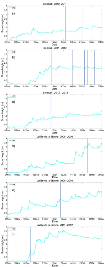
snow cover characteristics of all acquisitions for the basin ST. Snow depths in 2010/11 and 2012/13 were lower (be-tween 1.33 and 1.43 m) than in 2011/12, when snow depth varied between 1.91 and 2.75 m. The coefficient of variation ranges from 0.2 to 0.37 with generally increasing values to-wards the end of the accumulation period. Thus we believe it is a potentially good indicator for the increasing redistribu-tion of the snow cover during the accumularedistribu-tion season. Fig-ure 5 shows the evolution of snow depth for the three winter seasons of 2010/11, 2011/12 and 2012/13 at the weather sta-tion WAN7 in close vicinity to the basin ST. Interestingly, the maximum snow depth was reached very early in the winter season 2011/2012, in January, and it is basically the result of one long period of intermittent snowfalls. Normally peak ac-cumulations at these altitudes are reached later in the season (March or April).

At the Vallée de la Sionne test site, three ALS measure-ments were performed in three different winter seasons. The three scans were taken at significantly different stages of the accumulation season. Figure 5 shows the evolution of snow

Table 2. Mean HS, standard deviationσ (HS)and coefficient of variationCvof snow depth distribution for every laser scan

acqui-sition in the CB1 and CB2 basins.

Date HS[m] σ (HS)[m] Cv

Crêta Besse 1

8 Mar 2006 2.71 0.78 0.29

25 Jan 2009 1.36 0.64 0.47

8 Dec 2011 1.39 0.30 0.22

Crêta Besse 2

8 Mar 2006 3.68 0.61 0.17

25 Jan 2009 2.13 0.62 0.29

8 Dec 2011 1.36 0.23 0.17

depth for the winters 2005/06, 2008/09 and 2011/12 at the weather station Donin du Jour, which is situated about 2 km away from the basins. Table 2 shows the snow cover charac-teristics of all acquisitions for the basins CB1 and CB2. The scan acquired on 8 March 2006 can be considered close to the peak accumulation of the winter. The scan of 25 January 2009 is the result of several snowfalls within the winter sea-son. Both scans show a significantly larger standard devia-tion. Finally, the scan of the 8 December 2011 was performed after the first significant snowfall of the winter season, and represents a very homogeneous snowpack where little redis-tribution has taken place.

(7)

Fig. 5.Evolution of snow depth from 1 November until 31 March measured(a–c)at the weather station WAN7 in Steintälli and(d–f) at the weather station Donin du Jour in Vallée de la Sionne. The vertical blue lines correspond to the acquisition times of the laser scans.

Fig. 6. Terrain roughness derived from a DTM with 1 m resolu-tion, for a 5 m scale in(a)the ST basin and(b)the VdlS basin.

3.2 Terrain smoothing at basin scale

Figure 6 shows terrain roughness of the three basins CB1, CB2 and ST. We observe that the vector ruggedness measure

Rcaptures well terrain features such as rocky outcrops, boul-ders as well as small channels and gullies. It further confirms our selection criteria with increasing roughness from CB2 to ST to CB1. Mean roughness in CB2 is 0.0028 with a stan-dard deviation of 0.0044, mean roughness in ST is 0.0050 with a standard deviation of 0.0089, and mean roughness in CB1 is 0.0084 with a standard deviation of 0.133 (all values calculated at a scale of 5 m).

Figure 7 shows an example of the correlation between ter-rain roughness,RT, and snow surface roughness,RS, for the CB1 basin and for scales of 5 and 25 m. We observe a lin-ear relationship betweenRS and RT. Whereas the correla-tion is very strong at larger scales (R2 of 0.97 at a scale of 25 m), more deviation from the linear fit is observed on smaller scales (R2of 0.73 at a scale of 5 m).

Figure 8 gives an overview over all basins and showsF

(8)

Fig. 7.Snow surface roughness as a function of terrain roughness for every pixel in CB1 in the year 2011 for scales of(a)5 m and(b)25 m. In green the linear regression line.

and snow surface roughness as a function of different scales for the basins ST, CB1 and CB2. It confirms that correlation between terrain and surface roughness increases with scale in all basins. Further, all basins show a decreasing smooth-ing factor F with increasing scales. Thus, we observe in-versely proportional behaviour ofR2andF, indicating that the more terrain roughness is attenuated (highF), the more snow surface roughness can deviate from its underlying ter-rain, forming a distinct winter terrain (lowR2). This confirms quantitatively our intuitive understanding of terrain smooth-ing. We further observe that terrain smoothing is generally larger (higherF, lowerR2) in sampled basins with low ter-rain roughness (e.g CB2, Fig. 6). Smoothing is strongest in CB2 where small-scale terrain roughness could be almost completely eliminated (F close to 1,R2almost 0). With in-creasing terrain roughness (ST, CB1) terrain smoothing is less pronounced. This behaviour can be best illustrated with the example of 8 December 2011 in CB1 and CB2, where the first significant snowfall of the winter season resulted in a very similar mean snow depth (1.39 and 1.36 m in CB1 and CB2 respectively) in both basins. However, terrain smooth-ing is significantly larger (higherF, lowerR2) in CB2 than in CB1. This underlines that every basin has a unique imprint and shows a different smoothing behaviour even with almost identical snow depth distribution parameters such as mean snow depth.

Beside the basin characteristics, it is clear that the differ-ences of the smoothing behaviour observed within every in-dividual basin are due to a varying snow cover distribution.

Figure 8 shows qualitatively that terrain smoothing in-creases with increasing snow depth. In the basin ST for example, we clearly identify two different smoothing be-haviours between the two winters of 2010/11 and 2012/13 and the winter of 2011/12, which were characterized by snow depths in the range of 1.33–1.43 m and 1.91–2.75 m, respec-tively. This pronounced difference in snow depth of the win-ter season 2011/12 compared to the two others results in more pronounced smoothing at scales up to 15 m. At larger

scales,F of all winter seasons converges to values of around 0.45. However, this behaviour is not unequivocal, and mean snow depth alone cannot always explain terrain smoothing. For example, the scans of 11 January 2012 and 4 March 2012 show almost the same smoothing behaviour despite a signif-icantly larger mean snow depth on 11 January 2012 (2.75 m compared to 1.99 m on 4 March). In this case, the coefficient of variation,Cv, is significantly lower for the scan of 11 Jan-uary 2012, indicating that the snow cover is less distributed than for 4 March 2012. This is confirmed in other basins. In CB2 we observe that the smoothing in the year 2006 is only slightly larger than in 2009 despite a significantly thicker snowpack (3.68 m in 2006 compared to 2.13 m in 2009). Also in this case,Cv is almost twice as large in 2009, indicating that relatively more snow has been redistributed. In CB1 we observe that both years 2006 and 2009 show a very simi-lar smoothing behaviour despite higher mean snow depth in 2006. Again,Cvis larger in 2009; thus the snow cover was more affected by redistribution processes.

The above observations suggest that terrain smoothing may thus be dependent on the mean snow depth, HS, as well as its variability,σ (HS). To examine this relationship we use the data of the ST basin where eight laser scans are available. With only three scans in VdlS, this would not be possible. We define:

f

HS=HS×σ (HS)[m2]. (14)

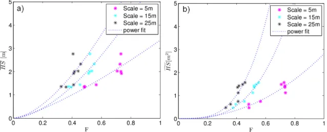
Figure 9 showsF withHS for the scales of 5, 15 and 25 mf and as a comparison only with HS. In both cases, we can see that increasing scales lead to a decreasing smoothing be-haviour and that a linear increase in HS and HS does notf result in a linear increase of the smoothing factor. Therefore a power function of the form

f

HS=c×Fr, (15)

(9)

(a) F in ST (b) F in CB1 (c) F in CB2

(d)R2_{in ST} _(e)R2_{in CB1} _(f)R2_{in CB2}

Fig. 8. (a–c)Smoothing factorF and (d–f)coefficient of determinationR2 (p <0.0001) between snow surface roughness and terrain roughness as a function of scale for the basins ST, CB1 and CB2.

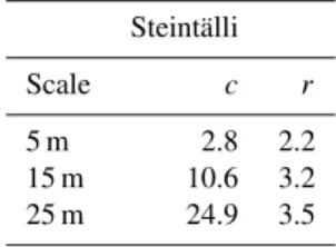
Table 3.Coefficientscandrof the power function modelling ter-rain smoothing (Eq. 16) in the basin of ST.

Steintälli

Scale c r

5 m 2.8 2.2

15 m 10.6 3.2

25 m 24.9 3.5

ofHS with F. Further, by visual inspection, we observe a bet-f ter agreement with the fit when the variability of snow depth is integrated.

If we solve Eq. (15) forF we obtain

F = HSf

c !1

r

, (16)

where Table 3 shows characteristic values ofcandrfor the basin ST.

The observed smoothing behaviour indicates that the snow which fell at the beginning of the winter season is more ef-ficient in cancelling out roughness than larger snowfalls

oc-curring later in the season, when the snow cover is already relatively high. Further, it shows how a simple standard de-viation can capture complex redistribution processes such as a wind transport, at least at basin scale.

We believe that the obtained relation in this basin captures well the essence of terrain smoothing. Basins with different terrain characteristics may show different behaviours with stronger or weaker increases ofF in relation to snow depth and its variability.

Nonetheless, this result suggests that, in contrast to the in-dications given by Schweizer et al. (2003), terrain smoothing processes are not restricted to snow depths of 0.3–1 m, but are still observable in considerably thicker snowpacks. How-ever, it is important to emphasize that this is dependent of the scale of terrain roughness under consideration. Consider-ing the work of Schirmer and LehnConsider-ing (2011), we can con-firm increasing terrain smoothing on increasing scales with a deeper and more variable snowpack; however we did not find a clear break separating scales where terrain is smoothed or not smoothed. We rather observe a gradual decrease of ter-rain smoothing with increasing scales.

(10)

Fig. 9. (a)F as a function of mean snow depth and(b)Fas a function of mean snow depth multiplied by its standard deviation for scales of 5, 15 and 25 m.

mostly between 5 and 10 m for snow depth ranging roughly between 1 and 3 m. Larger critical scales were found in smoother terrain of CB2 with values around 25 m. This find-ing is very useful to select appropriate resolutions of the DTM for modelling purposes in a winter terrain.

3.3 Terrain smoothing at local scale

As discussed above, terrain smoothing at basin scale is di-rectly proportional to the average snow depth and its standard deviation. However, to understand the smoothing behaviour of single terrain features, it is necessary to assess the link be-tween snow depth and surface roughness at local scale. Ac-cordingly, we analysed the correlation between snow depth and terrain smoothing at pixel scale (Fig. 10). This example shows that, in contrast to what was observed at basin level, it is not possible to establish a general relationship between the two variables. No relationship was found in any basin or at any scale.

To get a deeper understanding of this behaviour, we pro-duced gridded maps of 1 m resolution of snow depth and surface roughness and assessed the spatial distribution of snow depth and surface roughness. Figures 11 and 12 show two selected snow depth distributions and the correspond-ing surface roughness and underlycorrespond-ing terrain roughness at a scale of 5 and 25 m in the basin ST and VdlS, respec-tively. Maps of all snow depth and roughness distributions can be consulted in the Appendix. Even if a correlation be-tween snow depth and smoothing at the pixel level could not be found, by visual inspection we observe that snow can in-fluence smoothing processes at feature level, systematically and persistently. This can be observed for example in Fig. 11 where channels (marked with black circles) are systemati-cally filled with snow and completely disappear on the sur-face roughness maps, in all observed scans. Another example is surface roughness due to small rocks (marked with yellow

Fig. 10.Snow surface roughness as a function of snow depth for pixels with terrain roughness of 0.025±0.001. Example for acqui-sition of 2 February 2011 and a scale of 15 m in the basin ST.

(11)

8 Mar 2006 1

25 Jan 2009 0.58 1

8 Dec 2011 0.54 0.29 1

deposition, redistribution (e.g. snow drift, saltation, prefer-ential deposition (Lehning et al., 2008; Mott et al., 2010)) and/or wind erosion processes. Surface roughness might thus be influenced by drift features (dunes, cornices) or sastrugi. This complex behaviour is not captured by a simple power law as shown in Sect. 3.2, but can only be reproduced using physical models able to calculate snow redistribution in 3-D terrain (e.g. Alpine 3-D; Lehning et al., 2006).

However we stress that, under snow influence, character-istic patterns of surface roughness appear to be persistent. In the following we will thus analyse quantitatively the persis-tence of snow depth distribution and whether persispersis-tence is further transferred to surface roughness.

3.4 Intra- and interannual persistence of snow depth

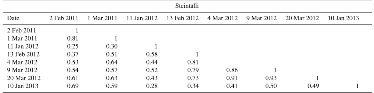
Table 5 shows the correlations of the snow depth distribution for the Steintälli basin. We observe high intra-annual corre-lation of 0.81 between the two scans in the season 2010/11 as well as the last four scans in 2011/12, with values ranging from 0.73 to 0.93. Only the scan from 11 January 2012 is cor-related to a less strong extent with all other scans from this winter season, with values ranging from 0.43 to 0.58. Thus, in general the intra-annual correlation at this site is strong, with higher values towards the middle and end of the accu-mulation season.

The same holds for the interannual comparison. The cor-relation between scans performed at the beginning of the winter season is generally lower as in the case of the scan from 11 January 2012 compared with the scan from 2 Febru-ary 2011 (R2=0.25) and with that from 10 January 2013 (R2=0.28). The correlation increases for scans performed towards the end of the winter season as in the case of scans from 1 March 2011 and 20 March 2012 (R2=0.65). Still, we observe that strong correlations exist also between scans acquired substantially before the peak of the accumulation season (e.g. scans of 10 January 2013 and 2 February 2011 with a correlation ofR2=0.69).

annual persistence (R2=0.58 between 2006 and 2009). To summarize, we generally observe larger intra- and in-terannual persistence for snow depth distributions acquired closer to the end of the accumulation period which have been exposed to settling and redistribution processes over a whole winter. Still, large persistence is possible already early in the accumulation season, under the condition that a cer-tain settling and redistribution has occurred (e.g. scans of 10 January 2013 and 2 February 2011 in ST). A significantly weaker intra- and interannual consistency was observed for snow depth distributions which resulted basically from the first snowfall or snowfall period in the winter season, like the scans from 11 January 2012 in ST or the scan from 8 De-cember 2011 in VdlS. Thus, a single snowfall (period) at the beginning of the accumulation season can considerably vary from the characteristic accumulation pattern.

This is in agreement with previous studies of the snow cover distribution, which have generally found very high in-terannual persistence of the snow cover at the end of the ac-cumulation season, with correlations up to 0.97 (Pearson’s correlation coefficient; Schirmer et al., 2011). Yet, interan-nual persistence is slightly lower in the Steintälli basin. This can be explained by large glide cracks in the winter sea-son 2011/12, affecting the snow depth distribution during the whole winter season. Still the correlations are significant and the results confirm the hypothesis that the snow cover distri-bution converges towards a site-specific, characteristic pat-tern.

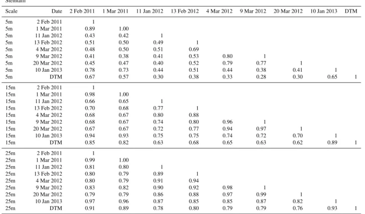
3.5 Intra- and interannual persistence of surface roughness

Tables 6 and 7 show the correlation of surface roughness of all winter surfaces with each other and with terrain roughness at scales of 5, 15 and 25 m for the basins ST, CB1 and CB2 respectively.

(12)

(a) DTM (b) 01 Mar 2011 (c) 20 Mar 2012

±

HS [m]

High : 4

Low : 0

0 3060 120 180 240

Meters

(d) 01 Mar 2011

±

HS [m]

High : 4

Low : 0

0 3060 120 180 240

Meters

(e) 20 Mar 2012

Fig. 11. (a)Surface roughness of summer terrain and(b, c)winter terrain at a scale of 5 m in the basin ST.(d, e)show the corresponding snow depth distributions. The black and yellow circles show persistent smoothing features. Red circles show the location of glide cracks.

Table 5.Coefficient of determination (R2) of correlations between snow depth distributions in the ST basin (p <0.0001).

Steintälli

Date 2 Feb 2011 1 Mar 2011 11 Jan 2012 13 Feb 2012 4 Mar 2012 9 Mar 2012 20 Mar 2012 10 Jan 2013

2 Feb 2011 1

1 Mar 2011 0.81 1

11 Jan 2012 0.25 0.30 1

13 Feb 2012 0.37 0.51 0.58 1 4 Mar 2012 0.53 0.64 0.44 0.81

9 Mar 2012 0.54 0.57 0.52 0.79 0.86 1

20 Mar 2012 0.61 0.63 0.43 0.73 0.91 0.93 1

10 Jan 2013 0.69 0.59 0.28 0.34 0.41 0.50 0.49 1

We observe that the persistence of snow surface roughness follows similar patterns to those observed for the snow depth distribution. For example, the intra-annual persistence at a scale of 5 m in ST in 2010/11 is slightly larger than those of the corresponding snow depth distribution (R2=0.89 com-pared to 0.81 for snow depth), whereas in 2011/12 the persis-tence is slightly weaker. The same is observed for the

(13)

±

03060 120 180 240

Meters

(a) DTM

±

03060 120 180 240

Meters

(b) 08 Mar 2006

±

03060 120 180 240

Meters

(c) 25 Jan 2009

HS [m]

High : 6

Low : 0

±

03060 120 180 240 Meters

(d) 08 Mar 2006

HS [m]

High : 6

Low : 0

±

03060 120 180 240 Meters

(e) 25 Jan 2009

Fig. 12. (a)Surface roughness of summer terrain and(b, c)winter terrain at a scale of 25 m in the basins CB1 and CB2.(d, e)show the corresponding snow depth distributions. Pixmaps©2013 swisstopo (5704 000 000).

surface roughness is similar to those of the snow depth distri-bution at a scale of 5 m, it is significantly higher for the larger scales of 15 and 25 m. Even more important, winter terrain roughness is correlated to a significantly larger degree with all other winter surfaces with similar or larger snow depth than each of the winter surfaces is with the terrain. For exam-ple, at a scale of 5 m in ST, an increase ofR2between 0.09 and 0.16 for all winter surfaces is observed using the win-ter win-terrain of 10 January 2013 as a reference instead of the summer terrain. This is noteworthy as several glide cracks in winter 2011/12 introduced considerable alteration in the surfaces. At larger scales of 15 and 25 m the increase is also observed but to a slightly lesser extent. This is mainly due to the already very strong correlation with the terrain at larger scales, reducing the potential gain in correlation.

The same behaviour can be observed in the basins CB1 and CB2. Using for example the scan of the first snowfall of the winter season on 8 December 2011 instead of the summer terrain increases the correlation with the surfaces of 8 March 2006 and 25 January 2009 of 0.1 and 0.23 respectively in CB1 (0.21 and 0.1 in CB2 respectively). In the case of CB2 the increase of correlation is even more pronounced on larger scales (15 and 25 m) than at the 5 m scale, with an increase ofR2up to 0.31. That confirms the finding in Sect. 3.3 that snow influence in smooth terrain affects larger scales than in rough terrain.

(14)

15m 2 Feb 2011 1

15m 1 Mar 2011 0.98 1.00

15m 11 Jan 2012 0.66 0.65 1

15m 13 Feb 2012 0.70 0.68 0.77 1

15m 4 Mar 2012 0.68 0.67 0.80 0.88

15m 9 Mar 2012 0.68 0.67 0.74 0.80 0.96 1

15m 20 Mar 2012 0.67 0.67 0.72 0.77 0.94 0.97 1

15m 10 Jan 2013 0.94 0.93 0.75 0.75 0.74 0.72 0.70 1

15m DTM 0.85 0.82 0.63 0.68 0.65 0.63 0.62 0.89 1

25m 2 Feb 2011 1

25m 1 Mar 2011 0.99 1.00

25m 11 Jan 2012 0.81 0.80 1

25m 13 Feb 2012 0.80 0.79 0.89 1

25m 4 Mar 2012 0.80 0.79 0.91 0.94

25m 9 Mar 2012 0.83 0.82 0.90 0.92 0.98 1

25m 20 Mar 2012 0.79 0.79 0.86 0.88 0.97 0.99 1

25m 10 Jan 2013 0.97 0.96 0.87 0.85 0.85 0.87 0.82 1

25m DTM 0.91 0.89 0.78 0.80 0.79 0.79 0.76 0.93 1

Table 7.Coefficient of determination (R2) of surface roughness correlations in the CB1 and CB2 basins (p <0.0001).

Crêta Besse 1 Crêta Besse 2

Scale Date 8 Mar 2006 25 Jan 2009 8 Dec 2011 DTM 8 Mar 2006 25 Jan 2009 8 Dec 2011 DTM

5m 8 Mar 2006 1 1

5m 25 Jan 2009 0.62 1 0.38 1

5m 8 Dec 2011 0.49 0.65 1 0.31 0.33 1

5m DTM 0.39 0.43 0.73 1 0.10 0.23 0.43 1

15m 8 Mar 2006 1 1

15m 25 Jan 2009 0.89 1 0.74 1

15m 8 Dec 2011 0.84 0.84 1 0.67 0.64 1

15m DTM 0.78 0.76 0.93 1 0.36 0.43 0.72 1

25m 8 Mar 2006 1 1

25m 25 Jan 2009 0.95 1 0.83 1

25m 8 Dec 2011 0.92 0.89 1 0.81 0.74 1

25m DTM 0.88 0.84 0.97 1 0.53 0.53 0.79 1

characteristics of a winter terrain surface, including wind ef-fects, without extensive modelling of the snow cover. How-ever, this is only true if the reference DSM is used to ap-proximate winter surfaces with similar or deeper snowpack. A DSM representing a very thick snow cover situation might be less representative for a thin snow cover situation than the summer DTM.

(15)

In this study we present a method to quantify terrain smooth-ing based on a multi-scale roughness approach. This method allows us to link terrain smoothing to geomorphological pa-rameters as the roughness estimates used in our study are based on changes in slope and aspect. Together with the pos-sibility to precisely map roughness changes in the terrain, this is a significant step forward in interpreting terrain smoothing. The analysis of three selected alpine basins suggests that, at basin scale, not only mean snow depth but also its vari-ability drive the process of terrain smoothing. The multi-temporal analysis in one basin revealed that the relation be-tween terrain smoothing and snow depth parameters follows a power law indicating that snowfalls at the beginning of the winter season are more efficient in eliminating terrain roughness than snowfalls occurring later in the season. On the other hand, a relationship between terrain smoothing and snow depth was not found at pixel level as geomorphology and snow depth of neighbouring pixels strongly influence surface roughness at a given point. Still, at larger scales, winter terrain roughness can be derived, even at pixel level, from a summer DTM using a simple smoothing factor as the relationship between terrain and snow surface roughness is strongly linear. At smaller scales, snow surface roughness decorrelates stronger from terrain roughness and the summer DTM is not representative for the winter surface anymore. In this case, the representation of a winter terrain can be sig-nificantly improved by the acquisition of a winter DSM with similar or less snow depth as it captures site-specific and per-sistent effects of wind–terrain interaction on the snow depth distribution.

Our results are promising; however, the relatively small number of data sets with limited spatial and temporal ex-tent restricts the generality of our results. A larger number of scans obtained in all possible snow cover situations, cover-ing different terrain types and snow climates, would be nec-essary to confirm and strengthen the significance of our find-ings. New technologies to derive high-resolution DSMs over a wide area even in a winter terrain are currently being de-veloped (Bühler et al., 2012; Bühler, 2012), making it more feasible in the future to obtain DSMs at significantly lower cost than lidar techniques.

Such winter terrains may then be very useful in avalanche dynamics simulations (e.g. RAMMS; Christen et al., 2010) as they provide a more realistic estimation of topography. For example the disappearance of small channels observed in a

determining avalanche release size and location. This has to be assessed in future studies. A more realistic winter terrain will further improve modelling of wind–ground interaction in snow-covered terrain and be important for better snow distribution simulation, which can be valuable for water re-sources assessment or ecology purposes.

Acknowledgements. Funding for this research has been provided through the Interreg project STRADA by the following partners: Amt für Wald Graubünden, Canton du Valais – Service de forêts et paysage, Regione Lombardia, ARPA Lombardia, ARPA Piemonte, and Regione Autonoma Valle d’Aosta. The authors would like to thank Walter Steinkogler for helping in the acquisition of the laser scans. We also thank the two reviewers, Margherita Maggioni and Samuel Morin, for their very constructive comments and corrections which considerably improved the manuscript.

Edited by: E. Larour

References

Blöschl, G.: Scaling issues in snow hydrology, Hydrol. Process., 13, 2149–2175, 1999.

Bühler, Y.: Remote sensing tools for snow and avalanche research, Proceedings of the 2012 International Snow Science Workshop, Anchorage, Alaska, 264–268, 2012.

Bühler, Y., Marty, M., and Ginzler, C.: High Resolution DEM Gen-eration in High-Alpine Terrain Using Airborne Remote Sensing Techniques, Transactions in GIS, 16, 635–647, 2012.

Bühler, Y., Kumar, S., Veitinger, J., Christen, M., Stoffel, A., and Snehmani: Automated identification of potential snow avalanche release areas based on digital elevation models, Nat. Hazards Earth Syst. Sci., 13, 1321–1335, doi:10.5194/nhess-13-1321-2013, 2013.

Christen, M., Kowalski, J., and Bartelt, P.: RAMMS: Numerical simulation of dense snow avalanches in three-dimensional ter-rain, Cold Reg. Sci. Technol., 63, 1–14, 2010.

Deems, J. S., Fassnacht, S. R., and Elder, K. J.: Fractal Distribution of Snow Depth from Lidar Data, J. Hydrometeorol., 7, 285–297, 2006.

Deems, J. S., Fassnacht, S. R., and Elder, K. J.: Interannual Consis-tency in Fractal Snow Depth Patterns at Two Colorado Mountain Sites, J. Hydrometeorol., 9, 977–988, 2008.

(16)

in a small mountain catchment, The Cryosphere, 4, 215–225, doi:10.5194/tc-4-215-2010, 2010.

Grünewald, T., Stötter, J., Pomeroy, J. W., Dadic, R., Moreno Baños, I., Marturià, J., Spross, M., Hopkinson, C., Burlando, P., and Lehning, M.: Statistical modelling of the snow depth distribution in open alpine terrain, Hydrol. Earth Syst. Sci., 17, 3005–3021, doi:10.5194/hess-17-3005-2013, 2013.

Hobson, R. D.: Surface roughness in topography: a quantitative ap-proach, 221–245, Harper & Row, 1972.

Horn, B. K. P.: Hill shading and the reflectance map, P. IEEE, 69, 14–47, 1981.

Lehning, M., Völksch, I., Gustafsson, D., Nguyen, T. A., Stähli, M., and Zappa, M.: ALPINE3D: a detailed model of mountain surface processes and its application to snow hydrology, Hydrol. Process., 20, 2111–2128, 2006.

Lehning, M., Löwe, H., Ryser, M., and Raderschall, N.:

In-homogeneous precipitation distribution and snow

trans-port in steep terrain, Water Res. Res., 44, W07404,

doi:10.1029/2007WR006545, 2008.

Lehning, M., Grünewald, T., and Schirmer, M.: Mountain

snow distribution governed by an altitudinal gradient

and terrain roughness, Geophys. Res. Lett., 38, L19504, doi:10.1029/2011GL048927, 2011.

Maggioni, M. and Gruber, U.: The influence of topographic param-eters on avalanche release dimension and frequency, Cold Reg. Sci. Technol., 37, 407–419, 2003.

Maggioni, M., Bovet, E., Dreier, L., Buehler, Y., Godone, D., Bartelt, P., M., F., Chiaia, B., and Segor, V.: Influence of summer and winter surface topography on numerical avalanche simula-tions, Proceedings of the 2013 International Snow Science Work-shop, Grenoble, France, 591–598, 2013.

Manninen, T., Anttila, K., Karjalainen, T., and Lahtinen, P.: Auto-matic snow surface roughness estimation using digital photos, J. Glaciol., 58, 993–1007, 2012.

McClung, D.: Characteristics of terrain, snow supply and forest cover for avalanche initiation caused by logging, Ann. Glaciol., 32, 223–229, 2001.

McClung, D. M. and Schaerer, P. A.: The Avalanche Handbook, Seattle, WA, the mountaineers Edn., 2002.

Mott, R., Schirmer, M., Bavay, M., Grünewald, T., and Lehning, M.: Understanding snow-transport processes shaping the mountain snow-cover, The Cryosphere, 4, 545–559, doi:10.5194/tc-4-545-2010, 2010.

Schirmer, M. and Lehning, M.: Persistence in intra-annual

snow depth distribution: 2. Fractal analysis of snow

depth development, Water Resour. Res., 47, W09517,

doi:10.1029/2010WR009429, 2011.

Schirmer, M., Wirz, V., Clifton, A., and Lehning, M.: Persis-tence in intra-annual snow depth distribution: 1. Measurements and topographic control, Water Resour. Res., 47, W09516, doi:10.1029/2010WR009426, 2011.

Schweizer, J., Bruce Jamieson, J., and Schneebeli, M.:

Snow avalanche formation, Rev. Geophys., 41, 1016,

doi:10.1029/2002RG000123, 2003.

Simenhois, R. and Birkeland, K. W.: The effect of changing slab thickness on fracture propagation, Proceedings of the 2008 In-ternational Snow Science Workshop, Whistler, B.C., 755–760, 2008.

Sovilla, B., McElwaine, J. N., Schaer, M., and Vallet, J.: Variation of deposition depth with slope angle in snow avalanches: Measure-ments from Vallée de la Sionne, J. Geophys. Res., 115, F02016, doi:10.1029/2009JF001390, 2010.

Sovilla, B., Sonatore, I., Bühler, Y., and Margreth, S.: Wet-snow avalanche interaction with a deflecting dam: field observa-tions and numerical simulaobserva-tions in a case study, Nat. Hazards Earth Syst. Sci., 12, 1407–1423, doi:10.5194/nhess-12-1407-2012, 2012.

Trujillo, E., Ramirez, J. A., and Elder, K. J.: Topographic, meteo-rologic, and canopy controls on the scaling characteristics of the spatial distribution of snow depth fields, Water Resour. Res., 43, W07409, doi:10.1029/2006WR005317, 2007.

Vallet, J.: Quick Deployment Heliborne Handheld LiDAR System for Natural Hazard Mapping, 3–7 May, in: Gi4DM – Geoinfor-mation for Disaster management Conference, Antalya, Turkey, 2011.

van Herwijnen, A. and Heierli, J.: Measurement of crack-face fric-tion in collapsed weak snow layers, Geophys. Res. Lett., 36, L23502, doi:10.1029/2009GL040389, 2009.

Vontobel, I.: Geländeanalysen von Unfalllawinen, Master’s thesis, Department of Geography, University of Zurich, 2011.

(h) 20 Mar 2012

Pixelkarten © XXXX (aktuelles J ahr) swiss topo (5704 000 000) 0 3060 120 180 240

Meters

±

Roughness

0 - 0.001 0.001 - 0.002 0.002 - 0.005 0.005 - 0.01 0.01 - 0.02 0.02 - 0.05 0.05 - 0.1 > 0.1

(h) 20 Mar 2012

0 3060 120 180 240 Meters

±

Roughness 0 - 0.001 0.001 - 0.002 0.002 - 0.005 0.005 - 0.01 0.01 - 0.02 0.02 - 0.05 0.05 - 0.1 > 0.1

(i) 10 Jan 2013

±

HS [m]

High : 4

Low : 0

0 3060 120 180 240 Meters

(g) 20 Mar 2012

0 3060 120 180 240 Meters

±

HS [m]

High : 4

Low : 0

(h) 10 Jan 2013

(21)

±

03060 120 180 240

Meters

(a) DTM

±

03060 120 180 240

Meters

(b) 08 Mar 2006

±

03060 120 180 240

Meters

(c) 25 Jan 2009

±

03060 120 180 240

Meters

(d) 08 Dec 2011

(22)

±

03060 120 180 240

Meters

(a) DTM

±

03060 120 180 240

Meters

(b) 08 Mar 2006

±

03060 120 180 240

Meters

(c) 25 Jan 2009

±

03060 120 180 240

Meters

03060 120 180 240 Meters

(c) 08 Dec 2011