MODIS Collection 6 shortwave-derived cloud phase classification algorithm and comparisons with CALIOP

(1)

Atmos. Meas. Tech., 9, 1587–1599, 2016 www.atmos-meas-tech.net/9/1587/2016/ doi:10.5194/amt-9-1587-2016

MODIS Collection 6 shortwave-derived cloud phase classification

algorithm and comparisons with CALIOP

Benjamin Marchant1,2, Steven Platnick1, Kerry Meyer1,2, G. Thomas Arnold1,3, and Jérôme Riedi4 1_{NASA Goddard Space Flight Center, Greenbelt, Maryland, USA}

2_{USRA Universities Space Research Association, Columbia, Maryland, USA} 3_{SSAI, Inc., 10210 Greenbelt Road, Lanham, MD 20706, USA}

4_{LOA (Laboratoire d’Optique Atmospherique), Université Lille 1, France}

Correspondence to:Benjamin Marchant ([email protected])

Received: 9 September 2015 – Published in Atmos. Meas. Tech. Discuss.: 16 November 2015 Revised: 22 February 2016 – Accepted: 12 March 2016 – Published: 11 April 2016

Abstract. Cloud thermodynamic phase (ice, liquid, unde-termined) classification is an important first step for cloud retrievals from passive sensors such as MODIS (Moder-ate Resolution Imaging Spectroradiometer). Because ice and liquid phase clouds have very different scattering and ab-sorbing properties, an incorrect cloud phase decision can lead to substantial errors in the cloud optical and micro-physical property products such as cloud optical thickness or effective particle radius. Furthermore, it is well estab-lished that ice and liquid clouds have different impacts on the Earth’s energy budget and hydrological cycle, thus ac-curately monitoring the spatial and temporal distribution of these clouds is of continued importance. For MODIS Col-lection 6 (C6), the shortwave-derived cloud thermodynamic phase algorithm used by the optical and microphysical prop-erty retrievals has been completely rewritten to improve the phase discrimination skill for a variety of cloudy scenes (e.g., thin/thick clouds, over ocean/land/desert/snow/ice surface, etc). To evaluate the performance of the C6 cloud phase algorithm, extensive granule-level and global comparisons have been conducted against the heritage C5 algorithm and CALIOP. A wholesale improvement is seen for C6 compared to C5.

1 Introduction

In addition to cloud height, thickness, and microphysics (e.g., size distribution), thermodynamic phase (i.e., ice, liq-uid, mixed) is an important determinant of the role of clouds

in the Earth’s radiation budget, weather, and hydrological cy-cle (Liou, 1986; Ramanathan et al., 1989, 2001; Chahine et al. 1992; Wielicki et al., 1995). Moreover, correctly deter-mining the phase of a cloudy field of view is a critical initial step for remote sensing retrievals of cloud properties such as optical thickness (COT), effective particle radius (CER), and water path. Because ice and liquid phase clouds have sub-stantially different scattering and absorption properties, an incorrect phase decision can lead to significant errors in re-motely retrieved cloud properties. For those reasons several cloud phase classification algorithms have been developed and continue to be improved for several instruments such as AVHRR (Key and Intrieri, 2000), CALIOP (Hu et al., 2009), POLDER (Goloub et al., 2000; Riedi et al., 2010), AIRS (Jin and Nasiri, 2014) and MODIS (Platnick et al., 2003; Baum et al., 2012). Each of these algorithms is designed to take advantage of the given instrument’s features; here we intro-duce the new cloud phase algorithm developed for MODIS Collection 6 (C6).

(2)

2003), designated MOD06 and MYD06 for Terra and Aqua, respectively (for simplicity, the Terra and Aqua products will be referred to collectively with the identifier “MOD” since the retrieval algorithms are the same for each platform). The MOD06 product includes 1 km pixel-level cloud ther-modynamic phase information derived from two approaches, namely an algorithm that exclusively uses infrared (IR) chan-nels (Baum et al., 2000, 2012) whose results are reported for both daytime and nighttime (also available at 5 km resolu-tion), and a daytime-only algorithm that uses a combination of visible (VIS), shortwave IR (SWIR), and IR channels.

The daytime-only algorithm (referred to hereafter as the MOD06 cloud optical property (COP) phase algorithm) that provides the phase decisions for the MOD06 cloud optical and microphysical property retrievals (e.g., COT, CER, cloud water path) has undergone an extensive overhaul in the latest MOD06 C6 reprocessing efforts. The primary motivation for the C6 changes was to overcome some well-known short-comings in Collection 5 (C5). In particular, the C5 phase decision logic was somewhat opaque to end users, and be-cause the algorithm relied on SWIR channel ratio thresh-olds specific to MODIS, was inadequate for achieving cli-mate data record continuity from multiple passive sensors such as MODIS, VIIRS, and beyond. In addition, the algo-rithm underperformed in certain situations, such as broken liquid cloud scenes that were often misidentified as ice and thin ice cloud edges that were often misidentified as liquid. Because the cloud phase decision determines the processing path (i.e., ice or liquid) of the MOD06 retrievals, an incorrect cloud phase classification can introduce substantial errors in the final Level-2 COT, CER and water path products. Fur-thermore, these errors can impact the global Level-3 prod-uct (MOD08) by introducing biases into the grid-level, phase segregated cloud property populations (e.g., ice and liquid phase fractions) and derived statistics.

With these shortcomings in mind, the design goals for the new C6 MOD06 COP phase algorithm were to create a more universal phase algorithm applicable to multiple sen-sors and to minimize cloud phase decision errors. Algo-rithm development relied heavily on collocated observations from CALIOP (Cloud-Aerosol Lidar with Orthogonal Po-larization) onboard CALIPSO (Winker et al., 2009), and a thorough assessment was performed using CALIOP as the benchmark. Notable changes include a complete restructur-ing of the phase decision logic, though some C5 tests were retained for C6, in addition to removal of the bulk of the SWIR ratio threshold tests in favor of assessments of ice and liquid phase spectral CER retrievals that inherently account for instrument differences (e.g., spectral channel selection and response functions, etc.). Here, a detailed description of the C6 MOD06 COP phase algorithm is provided, including changes and enhancements with respect to C5. The C6 phase algorithm compares quite well with CALIOP for scenes in which CALIOP observes only one cloud phase. Furthermore,

the C6 algorithm is shown to provide a significant perfor-mance improvement over C5 for all surface types.

2 Data

The active lidar observations from CALIOP provide an ex-cellent benchmark for developing and evaluating the C6 MOD06 COP phase algorithm. This study uses the CALIOP cloud phase discrimination (Hu et al., 2009) reported in the 1 and 5 km cloud layer products for two selected months (July 2008 and November 2012). First the CALIOP 1 km layer products are collocated with MODIS by finding the MODIS pixel with the minimum great circle distance with respect to each CALIOP profile. Because some optically thin clouds such as cirrus require lidar horizontal averaging scales longer than 1 km for detection and are only reported in the CALIOP 5 km layer products, the 5 km layer products are also col-located with MODIS by over-sampling the 5 km profiles to 1 km resolution and concatenating with the 1 km layer prod-ucts. Thus a complete CALIOP phase data set is created to screen for single-phase ice or liquid profiles only. The impor-tance of this merged data set is illustrated in Fig. 1. Here the CALIOP 1 (panel b) and 5 km (panel d) layer cloud phase, with dark and light blue denoting liquid and ice phases, re-spectively, is plotted for an example Aqua MODIS gran-ule observed on 3 July 2008 at 08:30 UTC (panel a). Also shown in Fig. 1b, d is a horizontal bar near 20 km altitude indicating the collocated MOD06 C6 cloud phase classifica-tion (panel c). It is evident here that the CALIOP 1 and 5 km cloud layer sampling can be quite different, with more low-altitude, broken liquid clouds found in the 1 km layer prod-uct and more high-altitude ice clouds found in the 5 km layer product. Note the CALIOP 333 m layer products were also evaluated, though only minor differences were found with respect to the 1 km products. Consequently, the 333 m layer products are excluded from this investigation.

3 Algorithm description

(3)

B. Marchant et al.: MODIS Collection 6 shortwave-derived cloud phase classification algorithm 1589

Figure 1.Aqua MODIS granule (3 July 2008, 08:30 UTC) with the corresponding RGB image(a)and the MODIS C6 cloud phase classifi-cation(c), selected to illustrate the collocation between MODIS and CALIOP 1 km(b)and 5 km(d)cloud layer products.

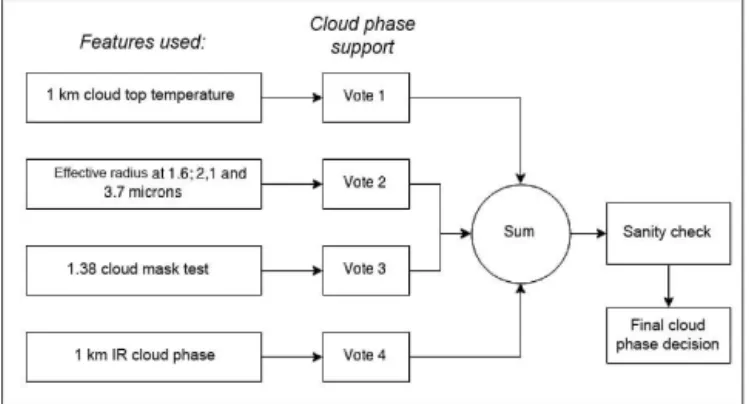
Figure 2.MODIS C6 cloud phase classification algorithm general logic flowchart.

For a given 1 km MODIS pixel, the COP cloud phase al-gorithm is only invoked if the pixel is classified as “cloudy” or “probably cloudy” by the MODIS cloud mask (MOD35),

(4)

3.1 Cloud top temperature tests

An obvious first-order cloud phase test is the application of thresholds on the retrieved cloud top temperature (CTT), here the new 1 km CTT product that is included in MOD06 (Baum et al., 2012). However, the MOD06 cloud top retrieval is known to lose sensitivity for optically thinner clouds, roughly below COT =2 (Menzel et al., 2010). Furthermore, for mul-tilayer scenes, namely ice clouds overlying liquid clouds that are often difficult to identify with passive imager-based tech-niques, a simple CTT threshold test may yield undesirable phase results. For instance, the cloud top retrieval may give a relatively cold CTT (e.g., less than 240 K) for moderately thick cirrus overlying an optically thick liquid cloud, and thus result in an ice phase vote, even though the underlying liquid cloud may dominate the TOA reflectance in the solar chan-nels; in such a case the more radiatively consistent result may instead be liquid phase. It is therefore important to exercise caution when determining cloud phase from CTT retrievals alone, and the CTT test was designed with these limitations in mind.

For optically thick warm clouds (i.e., liquid COT > 2 and CTT > 270 K), the CTT retrieval is considered to be of high confidence and the cloud phase is forced to liquid via an insurmountably large vote. This is analogous to the “warm sanity check” in the C5 algorithm. Conversely, for cold clouds (i.e., CTT < 240 K) the possibility of multi-layer (or mixed-phase) clouds precludes such confidence, and the test yields only a weak vote for ice phase. Optically thin warm clouds (COT < 2), or those clouds with a more ambiguous warm CTT retrieval (260 K < CTT < 270 K), yield weaker liquid phase votes. Completely ambiguous CTT retrievals (240 K < CTT < 260 K) yield no phase vote (i.e., undeter-mined).

3.2 Tri-spectral IR cloud phase test

As part of the MOD06 cloud top property retrieval algorithm, an IR-only cloud phase is also provided at 1 and 5 km resolu-tion. Previously a two-channel approach, for C6 this product was enhanced with the addition of a third IR channel (Baum et al., 2012), and uses emissivity ratios to infer cloud phase. While the bi-spectral IR cloud phase was used only as an initial guess in the C5 MOD06 COP phase algorithm, the so-called tri-spectral IR phase provides an independent vote in the C6 phase algorithm, albeit with a smaller weight since its results are strongly correlated with the retrieved CTT. Note in addition to ice, liquid, and undetermined designations, the tri-spectral IR phase can also return a mixed-phase desig-nation, though only the ice and liquid designations provide votes here.

3.3 1.38 µm channel test

To help identify optically thin cirrus as at the ice phase, a test based on the 1.38 µm channel is implemented in C6. An ad-vantage of the 1.38 µm channel is its location within a strong water vapor absorption band; if the atmosphere contains a sufficient amount of water vapor, measured TOA reflectance at 1.38 µm is primarily from high altitude cirrus that lie above most of the water vapor, while low altitude liquid clouds and the surface only negligibly contribute (Gao et al., 1993). The 1.38 µm test used in the COP cloud phase discrimination al-gorithm comes directly from the MODIS cloud mask product and is based on simple thresholds to separate thin cirrus from clear and low altitude clouds (Ackerman et al., 2010).

It should be noted that the skill of the 1.38 µm channel to discriminate ice and liquid clouds is strongly tied to the col-umn water vapor amount and the retrieved COT. For exam-ple, in more arid atmospheres (such as in subsidence zones), though optically thin low altitude clouds are still expected to negligibly contribute to TOA 1.38 µm reflectance, opti-cally thick low altitude liquid clouds may have a significant contribution. Thus applying the 1.38 µm test in all cases can lead to false ice cloud phase designations. Consequently, the 1.38 µm channel test is coupled with a retrieved ice phase COT threshold, and provides an ice phase vote only when retrieved COT is less than 2. Because the MOD06 COT re-trievals use solar window channels, and can thus be consid-ered total column retrievals, applying the 1.38 µm test only when COT is small adds confidence this test only votes ice phase for cirrus cases.

3.4 Spectral cloud CER tests

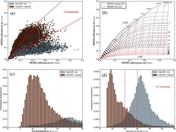
In C5, the primary COP cloud phase tests were a series of thresholds applied to SWIR reflectance ratios. The rationale for these tests is the fact that ice and liquid particles have different imaginary indexes of refraction at 1.6 and 2.1 µm (Kou et al., 1993); i.e., ice particles are more absorptive than liquid droplets at these wavelengths and thus have smaller TOA SWIR reflectances. Figure 3a shows a scatter plot of 2.1 µm (y axis) vs. 0.85 µm (x axis) cloud reflectances over ocean, randomly sampled from the MODIS–CALIOP collo-cated data set. The scatter point color indicates the collocollo-cated CALIOP cloud phase (ice phase in light blue and liquid phase in burgundy). The corresponding C5 SWIR ratio thresholds are plotted as dashed red lines, such that all points above the upper dashed red line are considered liquid and all points below the lower dashed red line are considered ice; points between the two lines are considered undetermined. It is evi-dent the SWIR ratio approach allows a rough discrimination of ice and liquid phase clouds, though the non-linearity of cloud reflectances, due to their dependence on COT, view geometry, etc., render single linear thresholds inadequate.

(5)

Figure 3.The MODIS C5 bidirectional reflectance thresholds(a)have been replaced by thresholds based on forced ice cloud effective radius (i.e., ice cloud effective radius retrieval is attempted for each cloudy pixel) retrieved at three separate wavelengths: 1.6, 2.1, and 3.7 µm. Example liquid (black) and ice (red) cloud retrieval look-up tables are shown in(b).(c)and(d)show the forced liquid and ice 2.1 µm cloud effective radius histograms, respectively, from the MODIS–CALIOP collocated data set, color coded by CALIOP-derived phase.

phase spectral CER retrievals (i.e., at 1.6, 2.1, and 3.7 µm) that inherently account for COT and view geometry (among other) dependencies. The rationale for this change is that it is more appropriate to define single linear thresholds in CER space than in reflectance space. Figure 3b shows example ice (red dashed line) and liquid (black dashed line) MOD06 COT–CER look-up tables (LUTs) for a given viewing ge-ometry. Note the C5 ice crystal model that assumed a mix-ture of crystal shapes has been replaced in C6 by a single-habit severely roughened aggregate column model (Yang et al., 2013) that provides better spectral consistency between MODIS solar- and IR-based COT retrievals as well as those from CALIOP (Holz et al., 2015). Figure 3c and d show histograms of forced liquid and ice phase 2.1 µm CER re-trievals along the CALIPSO track, respectively, segregated by collocated CALIOP phase (ice phase in light blue and liq-uid phase in burgundy). It is evident that the distribution of forced ice phase CER retrievals for those pixels identified as ice by CALIOP is quite different from that of the pixels identified as liquid; the forced liquid phase CER histograms are more ambiguous. Note, however, that including informa-tion about failed retrievals, i.e., from the new retrieval failure metric (RFM) introduced in C6 MOD06, can reduce the

am-biguity in the liquid phase CER histograms in Fig. 3c, though during development of the phase algorithm this information was not yet available. Similar results are found for the 1.6 and 3.7 µm CER retrieval histograms (not shown), though the 3.7 µm distributions are offset towards smaller CER com-pared to the 1.6 and 2.1 µm distributions. Thus it is possible to define simple CER thresholds to discriminate ice and liq-uid phase clouds; an example is shown by the dashed red lines in Fig. 3d. The C6 spectral CER thresholds were de-rived via extensive evaluation along the CALIPSO track with the collocated CALIOP cloud layer products, and are sum-marized in Table 1.

(6)

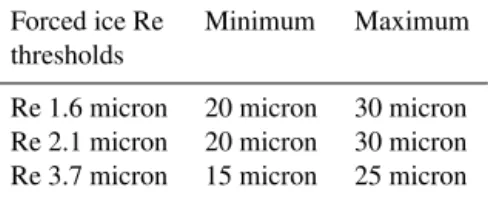
obser-Table 1. Forced ice cloud effective-radius-based thresholds (us-ing the severely roughened compact aggregated columns ice crys-tal model) derived from the MODIS–CALIOP collocated data set (Re < Min. liquid; Re > Max. ice; Max. > Re > Min. undetermined).

Forced ice Re Minimum Maximum thresholds

Re 1.6 micron 20 micron 30 micron Re 2.1 micron 20 micron 30 micron Re 3.7 micron 15 micron 25 micron

vations, as well as a measure of the relative distance to the LUT (note these parameters are reported for the final solu-tion phase in the RFM Scientific data sets (SDS). Thus for pixels for which any ice phase spectral CER retrieval fails, the C6 COP phase algorithm instead uses the nearest LUT CER information from the alternate solution logic. Note also that, because Aqua MODIS has non-functioning detectors at 1.6 µm, the 2.1 µm CER test is used as a proxy when 1.6 µm is not available, and therefore votes twice in such instances.

Finally, there are two distinct disadvantages to using spec-tral CER retrievals in the phase logic. First, computational efficiency is greatly reduced since it is necessary to perform two CER retrievals, i.e., both ice and liquid phase, for each of the three COT–CER spectral combinations (VNSWIR1.6, -2.1, -3.7 µm), thus six independent retrievals for each cloudy pixel. Second, the ice CER thresholds depend on the assumed ice crystal model used in the forward radiative transfer simu-lations. Therefore changes in the ice model assumption may in turn require changes in the CER thresholds.

4 Algorithm evaluation

To evaluate the performance of the C6 MOD06 COP phase algorithm, extensive comparisons have been carried out against the heritage C5 MOD06 algorithm, as well as col-located phase retrievals from the CALIOP v3 cloud layer products. In this section, we will first discuss the main differ-ences between C5 and C6 cloud phase results at a granule and global level. We will then discuss the CALIOP and MODIS cloud phase comparison results for a variety of surface types and cloud optical thicknesses, i.e., opaque and non-opaque clouds as determined by CALIOP.

4.1 Evaluation against C5

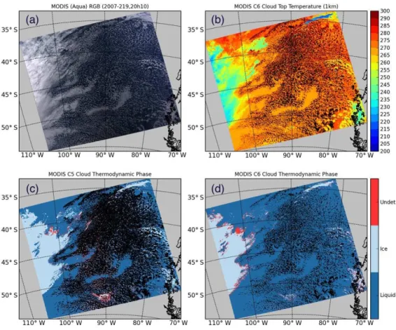
A comparison of cloud phase results from the C5 and C6 algorithms is shown in Fig. 4 for a selected Aqua MODIS granule observed on 7 August 2007 at 2010 UTC. Panel a shows the true color RGB image (0.66, 0.55, 0.47 µm) for this granule. The scene is mainly covered by broken marine boundary layer clouds and what appears to be cirrus on the left. Panel b shows the 1 km cloud top temperature retrievals,

and panels c and d show the C5 and C6 cloud phase classi-fication. Note the gray regions within the granule in panels b, c, and d correspond to clear sky pixels. Immediately visi-ble here is the increased number of cloud phase pixels in C6 compared to C5. This increase does not represent changes to the MOD35 cloud mask, but is instead a result of the inclu-sion in C6 MOD06 of pixels identified by the CSR algorithm as either cloud edges or partly cloudy (collectively referred to as PCL pixels) that are presumably inhomogeneous and were previously discarded in C5.

A research-level version of the C5 phase algorithm has been run on the PCL pixel population, and results indicate a large amount of the marine boundary layer clouds are mis-classified as ice phase (not shown). Broken liquid clouds such as those shown in Fig. 5 can be challenging for cloud phase classification for multiple reasons. For example, as can be seen in Fig. 5b, the CTT of broken clouds, particularly at higher latitudes, is often lower than the 270 K liquid phase threshold used in the C5 algorithm. Furthermore, inhomo-geneous broken clouds have been shown to be associated with a high CER retrieval failure rate (Zhang and Platnick, 2011; Cho et al., 2015); thus relying heavily on CER tests for phase determination can be problematic. Consequently, an extensive granule-level analysis was used to optimize the vote weights and CTT thresholds in the C6 COP phase al-gorithm to increase the classification skill for these clouds. These modifications helped to improve the cloud phase clas-sification, as the additional, likely inhomogeneous, PCL pix-els in the broken boundary layer cloud field in Fig. 5d are correctly classified as liquid. Finally, also note that C6 un-determined cloud phase (red color) is mainly reported in the transition between ice and liquid clouds, as we can expect in this ambiguous cloud phase area where multi-layer clouds might be found.

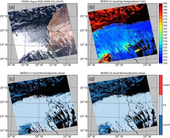
Cloud phase classification improvement can also be ob-served for C6 compared to C5 at the edge of cirrus clouds, especially over desert surfaces, as is shown by the Aqua MODIS granule (15 January 2008, 14:35 UTC) in Fig. 5. The RGB in Fig. 5a indicates a cirrus cloud deck extending from the tropical eastern Atlantic over the western Sahara. The corresponding MOD06 1 km CTT retrievals are shown in Fig. 5b, confirming the clouds are at high altitudes. It is ev-ident in Fig. 5c that the edges of the cirrus over the desert in this granule were misclassified in C5 as liquid phase clouds; this misclassification is greatly reduced for C6, shown in Fig. 5d.

The granule-level differences between C5 and C6 ob-served in Figs. 4 and 5 can also be obob-served in global sta-tistical aggregations. As an example, Fig. 6 shows MODIS C6 monthly liquid (panel a) and ice (panel b) cloud fraction (including both successful and unsuccessful optical property retrievals) gridded at 1×1◦

(7)

Figure 4.Example Aqua MODIS granule (7 August 2007, 20:10 UTC) with the corresponding RGB image(a), the C6 1 km cloud top temperature(b), and the cloud phase classification for C5(c)and C6(d), respectively. Note that for C6 the cloud phase is now reported for partially cloudy pixels leading to an increase of liquid cloud pixels, in particular for the broken cloud area.

population (i.e., CSR=1, 3) are shown in panels c and d, respectively. One can see that the PCL pixel population is mostly identified as liquid by the C6 COP phase algorithm, an expected result given that liquid clouds tend to be smaller in scale and have a more broken structure than do ice clouds. The difference between the C5 and C6 November 2012 monthly fractions, for the overcast CSR=0 pixel population only (PCL pixels were previously discarded in C5), is shown in Fig. 6e and f for liquid and ice phase, respectively. Here red shades indicate an increase for C6 over C5, and blue col-ors indicate a decrease; color bar values denote absolute frac-tion changes. Several differences are worth noting. The most obvious is that the C6 algorithm identifies more liquid phase clouds in the southern oceans than does C5, along with a cor-responding decrease in ice phase. An increase in liquid phase identification over many non-polar vegetated land areas, as well as a decrease over South America, is also evident. Com-parisons have also been performed for other months (e.g., summer months), with similar differences observed. As will be shown in subsequent sections, these C6 changes largely represent phase classification improvements over C5.

Although the C6 COP phase classification algorithm is significantly improved over C5, some situations continue to

be problematic. For instance, optically thin cirrus over warm surfaces, a particularly acute problem in C5 in which such cases were often incorrectly identified as liquid phase, may continue to be identified as liquid phase though C6 provides better skill in such circumstances, as shown in Fig. 5. In ad-dition, at oblique sun angles, especially at high latitudes, the spectral CER tests become less sensitive to phase and may incorrectly vote for liquid phase clouds. False ice phase clas-sification of broken liquid phase clouds also remains prob-lematic despite improvements in low maritime broken cloudy scenes. However, these pixels are often identified as partly cloudy by the CSR algorithm and are therefore excluded from the standard MOD06 retrieval products (though they are reported in separate PCL SDSs).

4.2 Evaluation against CALIOP

(8)

regard-Figure 5.Same as Fig. 4, except for an Aqua MODIS granule on 15 January 2008 (14:35 UTC). Note here the improvement of ice cloud edge classification over desert surface.

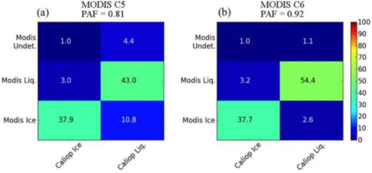
less of the success/failure status of the various spectral CER retrievals; the CSR=_{0 constraint is applied such that the C6} pixel population is consistent with C5. The abscissa denotes CALIOP phase, and the ordinate denotes MODIS phase. The numerical values in each table can be interpreted as the per-cent of total collocated cloudy scenes for which the given phase condition is observed. For instance, the value corre-sponding to the second column and second row in the C6 ta-ble (panel b) indicates that MODIS and CALIOP agreed on liquid phase designation in 54.4 % of the collocated cloudy pixels; similarly, the value of the first column and second row indicates that in 3.2 % of the collocated cloudy pixels CALIOP determined ice phase while MODIS disagreed, de-termining liquid phase. Note the total CALIOP ice and liq-uid phase populations, in terms of percent of the total col-located cloudy pixel population, can be found by summing each column; likewise, the MODIS ice, liquid, and undeter-mined phase populations are found by summing each row.

A convenient method of summarizing these contingency tables is to define a simple skill score, referred to as the phase agreement fraction (PAF): PAF=a2P,2+a3,1

i,j

ai,j

!

.

Here, the a values are the number of pixels correspond-ing to the phase condition of rowiand columnj. Thus the

(9)

Figure 6. Monthly gridded cloud phase fractions derived from the MOD06 COP phase product for November 2012.(a)and(b) show the liquid and ice cloud fraction, respectively, for the overcast (CSR=0) pixel population, while(c)and(d)show the partly cloudy PCL (CSR=1, 3) liquid and ice cloud fraction, respectively. The differences between the C5 and C6 overcast liquid(e)and ice(f)cloud phase fractions are also shown.

Figure 7.Contingency tables corresponding to MODIS C5(a)and C6(b)cloud phase calculated from the MODIS and CALIOP col-located data set during November 2012.

but may also be due to insufficiently screening out all multi-layer cloud cases from the MODIS–CALIOP collocated data set. In some cases where ice clouds overlap optically thick liquid clouds, CALIOP might detect only the overlying ice

cloud, while MODIS may identify the scene as liquid. This “spurious” liquid phase classification might in fact be prefer-able for the MODIS cloud optical products, as a liquid phase may provide better radiative consistency and reduce retrieval errors.

In addition to the contingency tables that globally sum-marize the cloud phase classification skill, a more detailed analysis has also been done. Figure 8 shows the global grid-ded November 2012 PAF score at 10×₁₀◦ _{resolution for} MODIS C5 (panel a) and C6 (panel b). The C6 cloud phase improvement is broadly distributed, with a noticeable im-provement over ocean. Moreover, the C5 cloud phase skill gradually decreased with increasing latitude, with a pro-nounced minimum over Antarctica, a shortcoming that has been greatly reduced in C6.

(10)

Figure 8.Gridded PAF (phase agreement fraction) score maps, for C5(a)and C6(b), obtained from the MODIS–CALIOP collocated data set for November 2012.

10 for November 2012 and July 2008, respectively. These fig-ures underscore the broad phase identification skill improve-ment for C6. Only for optically thin (non-opaque) clouds over desert surfaces, specifically in November 2012, does C6 slightly underperform C5; however, it should be noted the pixel count in this category is only 5 % of the total Novem-ber 2012 collocated cloudy pixel population. It is also worth noticing the significant improvement of the cloud phase skill over snow/ice surfaces for optically thick clouds compared to C5, in particular in November 2012. As expected, the cloud phase skill is overall lower for optically thin clouds compared to thick clouds, though C6 performs reasonably well for op-tically thin clouds over ocean.

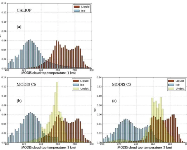
Cloud top temperature is a widely used parameter and plays a critical role in the MODIS cloud phase algorithm. Figure 11 shows the probability density functions (PDFs) for CALIOP (panel a) and MODIS C6 (panel b) and C5 (panel c) cloud phase against the MODIS 1 km cloud top temperature calculated for November 2012. Note these distributions again exclude multi-phase scenes as identified by CALIOP (about 20 % of cloudy scenes from the MODIS–CALIOP collocated data set present multi-phase scenes). The main conclusion is that the MODIS C6 ice and liquid PDFs now look quite similar to the CALIOP cloud phase PDFs, in contrast to C5

Figure 9.Detailed PAF (phase agreement fraction) scores, derived from the MODIS–CALIOP collocated data set for November 2012, as a function of surface type (ocean, snow/ice, desert, and vegetated land) and cloud opacity (opaque vs. non-opaque clouds) as deter-mined by CALIOP. The percentage of pixels for each classification is also shown (Note that coastal surfaces are not included).

Figure 10.Same as Fig. 9 except the month is July 2008.

that yields too much ice in the interval (240 K, 260 K). This figure also shows that the C6 undetermined cloud phase is roughly in the interval between 240 and 270 K, as expected since cloud phase discrimination is particularly difficult in these temperature ranges.

5 Conclusions

(11)

Figure 11.Probability density functions (PDFs) of CALIOP(a)and MODIS C6(b)and C5(c)cloud phase against the MODIS 1 km cloud top temperature for November 2012.

using intensive comparisons between MODIS and CALIOP. The new algorithm is now based on a simple majority vote logic that uses thresholds derived from MODIS and CALIOP comparisons instead of the C5 decision-tree-logic-based al-gorithm approach that was difficult to optimize. In addition, the C6 phase algorithm uses four primary tests, based on the 1 km cloud top temperature, the 1 km IR cloud phase, the 1.38 cirrus detection test from the MOD35 cloud mask, and three spectral cloud effective radius tests (derived from 1.6, 2.1, and 3.7 µm channels). The spectral effective radius tests effectively replace the C5 SWIR bidirectional reflectance ra-tio thresholds; the C5 SWIR rara-tio thresholds were problem-atic as they did not account for the reflectance dependence on both the viewing geometry and cloud optical thickness, lead-ing in particular to false ice phase classification for optically thick clouds. The new cloud effective radius tests outperform the C5 reflectance ratio tests, though the radius thresholds now depend on the assumed ice radiative model and are more computationally expensive.

These cloud phase classification algorithm modifications have resulted in noticeable changes between C5 and C6. In particular, global MODIS–CALIOP cloud phase classifica-tion agreement has increased by about 10 % for C6 com-pared to C5, leading to a total cloud phase agrement

be-tween MODIS C6 and CALIOP of over 90 % for single-phase cloudy pixels. Moreover, these improvements are ob-served for several surface types (ocean, land, desert, and snow/ice) and cloud optical thicknesses (thin and thick). The most significant improvement is found for opaque clouds (defined by the CALIOP lidar) over snow/ice surfaces. On the other hand, cloud phase discrimination for optically thin clouds over really bright or warm surfaces (such as thin cir-rus clouds over desert) continue to be problematic. Another important difference between C5 and C6, though not a result of cloud phase algorithm development, is the cloudy pixel population for which the cloud phase is reported. Previously in C5, only pixels identified as overcast by the clear sky restoral algorithm were optical/microphysical retrieval can-didates, and as such cloud phase was only reported for this pixel population (regardless of retrieval success/failure). For C6, optical/microphysical retrievals are also attempted for pixels classified as very inhomogenous (e.g., partly cloudy) and cloud phase is reported for this pixel population as well (again regardless of retrieval success/failure).

(12)

which CALIOP observed a single cloud phase in the column, the extent to which the results presented here hold for mul-tilayer clouds is still an open question. Limiting the anal-ysis to the CALIPSO ground track also limits the viewing and scattering angle space such that it is unclear whether the C6 improvements are consistent across the entire MODIS swath; the impacts of potential view angle dependencies are at present unknown. Moreover, because spectral channels sets can vary between satellite sensors (e.g., MODIS 2.1 µm vs. VIIRS 2.25 µm), it is uncertain whether the spectral ef-fective radius tests, as used here, can be applied uniformly across multiple platforms for climate data record continu-ity, though work to this end is ongoing. Nevertheless, the C6 COP phase algorithm represents a vast improvement over C5, and future work will focus on the remaining challenges such as multilayer clouds and view and scattering angle dependen-cies.

Data availability

MODIS data are available through the LAADS (Level 1 and Atmosphere Archive and Distribution Sys-tem) web http://modis-atmos.gsfc.nasa.gov/_docs/ C6MOD06OPUserGuide.pdf. Availability: from 2000 (Terra) and 2002 (Aqua) to today.

Edited by: B. Mayer

The Supplement related to this article is available online at doi:10.5194/amt-9-1587-2016-supplement.

References

Ackerman, S., Frey, R., Strabala, K., Liu, Y., Gumley, L., Baum, B., and Menzel, P.: Discriminating clear-sky from cloud with MODIS algorithm theoretical basis document (MOD35), ATBD reference number ATBDMpaych-OD-06, 129 pp., 2010. Baum, B. A., Soulen, P. F., Strabala, K. I., King, M. D.,

Acker-man, S. A., Menzel, W. P., and Yang, P.: Remote sensing of cloud properties using MODIS airborne simulator imagery dur-ing SUCCESS 2, Cloud thermodynamic phase, J. Geophys. Res., 105, 11781–11792, 2000.

Baum, B. A., Menzel, W. P., Frey, R. A., Tobin, D. C., Holz, R. E., Ackerman, S. A., Heidinger, A. K., and Yang, P.: MODIS cloud top property refinements for Collection 6, J. Appl. Meteorol. Cli-matol., 51, 1145–1163, 2012.

Chahine, M. T.: The hydrological cycle and its influence on climate, Nature, 359, 373–379, 1992.

Gao, B.-C., Goetz, A. F., and Wiscombe, W. J.: Cirrus cloud detec-tion from airborne imaging spectrometer data using the 1.38 µm water vapor band, Geophys. Res. Lett., 20, 301–304, 1993. Gao, B.-C., Goetz, A. F. H., Westwater, E. D. R., Conel J. E., and

Green, R. O.: Possible Near-IR Channels for Remote Sensing

Precipitable Water Vapor from Geostationary Satellite Platforms, J. Appl. Meteorol., 32, 1791–1801, 1993.

Goloub, P., Herman, M., Chepfer, H., Riedi, J., Brogniez, G., Cou-vert, P., and Seze, G.: Cloud thermodynamical phase classifica-tion from the POLDER spaceborne instrument, 39, 105, 14747– 14759, 2000.

Holz, R. E., Platnick, S., Meyer, K., Vaughan, M., Heidinger, A., Yang, P., Wind, G., Dutcher, S., Ackerman, S., Amarasinghe, N., and Wang, C.: Resolving cirrus optical thickness biases between CALIOP and MODIS using infrared retrievals, Atmos. Chem. Phys. Discuss., 15, 29455–29495, 2015.

Hu, Y., Winker, D., Vaughan, M., Lin, B., Omar, A., Trepte, C., Flittner, D., Yang, P., Nasiri, S. L., Baum, B., Sun, W., Liu, Z., Wang, Z., Young, S., Stamnes, K., Huang, J., Kuehn, R., and Holz, R.: Calipso/caliop cloud phase discrimination algorithm, J. Atmos. Ocean. Technol., 26, 2293–2309, 2009.

Jin, H. and Nasiri, S. L.: Evaluation of AIRS Cloud-Thermodynamic-Phase Determination with CALISO, J. Appl. Meteorol. Climatol., 53, 1012-1027, 2014.

Justice, C. O., Vermote, E., Townshend, J. R. G., Defries, R., and Roy, D. P.: The Moderate Resolution Imaging Spectroradiometer (MODIS): Land Remote Sensing for Global Change Research, IEEE Trans. Geosci. Remote Sens., 36, 1228–1249, 1998. Key, J. R. and Intrieri, J. M.: Cloud Particle Phase Determination

with the AVHRR, Notes and Correspondence, 1797–1804, 2000. King, M. D., Menzel, W. P., Kaufman, Y. J., Tanreì, D., Gao, B. C., Platnick, S., Ackerman, S. A., Remer, L. A., Pincus, R., and Hubanks, P. A.: Cloud and aerosol properties, precipitable water, and profiles of temperature and humidity from MODIS, IEEE Trans. Geosci. Remote Sens., 41, 442–458, 2003.

King, M. D., Platnick, S., Hubanks, P. A., Arnold, G. A., Moody, E. G., Wind, G., and Wind, B.: Collection 005 Change Summary for the MODIS Cloud Optical Properties (06-OD) Algorithm, 2006. Kou, L., Labrie, D., and Chylek, P.: Refractive indices of water and ice in the 0.65- to 2.5-µ m spectral range, Appl. Opt., 32, 3531– 3540, 1993.

Liou, K. N.: Influence of cirrus clouds on weather and climate pro-cesses: A global perspective, Mon. Weather Rev., 114, 1167– 1199, 1986.

Menzel, W. P., Frey Richard, A., and Baum, B. A.: Cloud top properties and cloud phase algorithm theoretical basis document, 2010.

Pincus, R., Platnick, S., Ackerman, S. A., Hemler, R. S., and Hof-mann, R. J. P.: Reconciling simulated and observed views of clo-dus: MODIS, ISCCP, and the limits of instrument simulators, J. Climate, 25, 4699–4720, doi:10.1175/JCLI-D-11-00267.1, 2012. Platnick, S., King, M. D., Ackerman, S. A., Menzel, W. P., Baum, B. A., Riedi, J. C., and Frey, R. A.: The MODIS cloud products: al-gorithms and examples from Terra, IEEE Trans. Geosci. Remote Sens., 41, 459–473, 2003.

Platnick, S., King, M. D., Meyer, K. G., Wind, G., Amarasinghe, N., Marchant, B., Arnold, G. T., Zhang, Z., Hubanks, P. A., Ridg-way, B., and Riedi, J.: MODIS Cloud Optical Properties: User Guide for the Collection 6 Level-2 MOD06/MYD06 Product and Associated Level-3 Datasets, http://modis-atmos.gsfc.nasa.gov/ _docs/C6MOD06OPUserGuide.pdf, 2014.

(13)

Re-B. Marchant et al.: MODIS Collection 6 shortwave-derived cloud phase classification algorithm 1599

sults from the Earth Radiation Budget Experiment, Research Ar-ticles, 243, 57–63, 1989.

Ramanathan, V., Crutzen, P. J., Kiehl, J. T., and Rosenfeld, D.: Aerosols, climate, and the hydrological cycle, Science, 294, 2119–2124, 2001.

Riedi, J., Marchant, B., Platnick, S., Baum, B. A., Thieuleux, F., Oudard, C., Parol, F., Nicolas, J.-M., and Dubuisson, P.: Cloud thermodynamic phase inferred from merged POLDER and MODIS data, Atmos. Chem. Phys., 10, 11851–11865, doi:10.5194/acp-10-11851-2010, 2010.

Wielicki, B. A., Cess, R. D., King, M. D., Randall, D. A., and Har-rison, E. F.: Mission to planet earth: role of clouds and radiation in climate, Bull. Am. Meteor. Soc., 76, 2125–2153, 1995.

Winker, D. M., Vaughan, M. A., Omar, A. H., Hu, Y., Powell, K. A., Liu, Z., Hunt, W. H., and Young, S. A.: Overview of the CALIPSO mission 85 and CALIOP data processing algorithms, J. Atmos. Ocean. Technol., 26, 2310–2323, 2009.

Yang, P., Bi, L., Baum, B. A., Liou, K. N., Kattawar, G. W., Mishchenko, M. I., and Cole, B.: Spectrally consistent scatter-ing, absorption, and polarization properties of atmospheric ice crystals at wavelengths from 0.2 to 100 µm, J. Atmos. Sci., 70, 330–347, 2013.