An objective determination of optimal site locations for detecting expected trends in upper-air temperature and total column ozone

(1)

ACPD

15, 1617–1650, 2015

An objective determination of optimal site locations

K. Kreher et al.

Title Page

Abstract Introduction

Conclusions References

Tables Figures

◭ ◮

Back Close

Full Screen / Esc

Printer-friendly Version Interactive Discussion

Discussion

P

a

per

|

Discussion

P

a

per

|

Discussion

P

a

per

|

Discussion

P

a

per

|

Atmos. Chem. Phys. Discuss., 15, 1617–1650, 2015 www.atmos-chem-phys-discuss.net/15/1617/2015/ doi:10.5194/acpd-15-1617-2015

This discussion paper is/has been under review for the journal Atmospheric Chemistry and Physics (ACP). Please refer to the corresponding final paper in ACP if available.

An objective determination of optimal site

locations for detecting expected trends in

upper-air temperature and total column

ozone

K. Kreher1,2, G. E. Bodeker1, and M. Sigmond3

1

Bodeker Scientific, Alexandra, New Zealand

2

BK Scientific, Mainz, Germany

3

Canadian Centre for Modelling and Analysis, Victoria, BC, Canada

Received: 27 October 2014 – Accepted: 5 December 2014 – Published: 19 January 2015 Correspondence to: K. Kreher ([email protected])

(2)

ACPD

15, 1617–1650, 2015

K. Kreher et al.

Title Page

Tables Figures

◭ ◮

Back Close

Full Screen / Esc

Discussion

P

a

per

|

Discussion

P

a

per

|

Discussion

P

a

per

|

Discussion

P

a

per

|

Abstract

In the first study reported on here, requirements on random uncertainty of instan-taneous temperature measurements, sampling frequency, season and pressure, re-quired to ensure a minimum random uncertainty of monthly mean temperatures, have been explored. These results then inform analyses conducted in a second study which

5

seeks to identify the optimal location of sites for detecting projected trends in upper-air temperatures in the shortest possible time. The third part of the paper presents a simi-lar analysis for the optimal locations of sites to detect projected trends in total column ozone. Results from the first study show that only for individual measurement random uncertainties >0.2 K does the measurement random uncertainty start to contribute

10

significantly to the random uncertainty of the monthly mean. Analysis of the effects of the individual measurement random uncertainty and sampling strategy on the ability to detect upper-air temperature trends shows that only when the measurement random uncertainty exceeds 2 K, and measurements are made just once or twice a month, is the quality of the trend determination compromised.

15

The time to detect a trend in some upper-air climate variable is a function of the unforced variance in the signal, the degree of autocorrelation, and the expected mag-nitude of the trend. For middle tropospheric and lower stratospheric temperatures, the first two quantities were derived from Microwave Sounding Unit (MSU) and Advanced Microwave Sounding Unit (AMSU) measurements while projected trends were obtained

20

by averaging 21st century trends from simulations made by 11 chemistry–climate mod-els (CCMs). For total column ozone, variance and autocorrelation were derived from the Bodeker Scientific total column ozone database with projected trends obtained from median values from 21 CCM simulations of total column ozone changes over the 21st century. While the optimal sites identified in this analysis for detecting temperature and

25

(3)

ACPD

15, 1617–1650, 2015

K. Kreher et al.

Title Page

Tables Figures

◭ ◮

Back Close

Full Screen / Esc

Discussion

P

a

per

|

Discussion

P

a

per

|

Discussion

P

a

per

|

Discussion

P

a

per

|

initiating measurement programmes at these sites or, if already in operation, to con-tinue to be supported.

1 Introduction

Stratospheric temperatures represent the first order connection between natural and anthropogenically driven changes in radiative forcing and changes in other climate

5

variables at the Earth’s surface. There is, therefore, a strong interest in detecting upper-air temperature trends as efficiently and reliably as possible. The vertical structure of temperature trends also provides important information for climate change attribution since increases in atmospheric long-lived greenhouse gas (GHG) concentrations warm the troposphere, but cool the stratosphere. Ozone also acts as a GHG and absorbs UV

10

radiation in the stratosphere such that changes in ozone concentration also change the temperature structure of the atmosphere. Thus, dependable long-term measurements of temperature and ozone are essential for climate change detection and attribution studies.

Historical observations present challenges for estimating trends since measurement

15

uncertainties can be large. A number of papers (e.g. Free et al., 2002; Wang et al., 2012 and references therein) point to the inherent, and partly irreparable, problems that arise from complicated merging of data sets of changing or unknown quality and different measurement approaches. Homogenisation of merged data sets cannot eliminate the respective uncertainty in derived trends.

20

Although satellite instruments are capable of measuring the vertical distribution of temperature and ozone globally, the resultant measurement series are often deficient for trend detection since: (1) the calibration of satellites, once in orbit, is a challenging task and slight differences in instrumental design, satellite and satellite-operation de-sign, and retrieval algorithms impose severe difficulties on constructing homogeneous

25

(4)

ap-ACPD

15, 1617–1650, 2015

K. Kreher et al.

Title Page

Tables Figures

◭ ◮

Back Close

Full Screen / Esc

Discussion

P

a

per

|

Discussion

P

a

per

|

Discussion

P

a

per

|

Discussion

P

a

per

|

propriate continuity or overlap in observations. (3) The vertical and horizontal resolution of satellite measurements may be too coarse to allow for appropriate interpretation and attribution of observed changes.

Stable ground-based long-term temperature and ozone measurements at selected sites, adhering to stringent measurement standards and traceability protocols (e.g.

5

Immler et al., 2010), facilitate the calibration of individual satellite instruments (e.g. Tobin et al., 2006; Balis et al., 2007; Adams et al., 2013) and support the merging of data sets from different satellites with the goal of creating reliable long-term climate data records (e.g. Tummon et al., 2014 and references therein). Such high-quality tem-perature and ozone time series can also support bridging any gaps that may emerge

10

in satellite data records. With unexpected termination of satellite operations, as well as the ongoing change in satellite technology, bridging gaps becomes critical to creating a continuous monitoring system for the global atmosphere.

More importantly though, these data sets could allow trend analysis in their own right. If observing sites are strategically placed, they might well sample a sufficiently

15

diverse range of regimes to provide a global picture of trends. Most of the current measurement sites, however, are located close to populated areas for ease of access and for historical reason. With approximately 90 % of the global population living in the Northern Hemisphere, measurement sites favour the Northern Hemisphere. As a result, such a distribution of sites is unlikely to be representative of the global climate.

20

An example for this is the distribution of the 15 initial GRUAN (GCOS Reference Upper-Air Network) sites which were predominantly located at Northern Hemisphere mid-latitudes (see map at www.gruan.org). Hence, the need exists to provide an objective approach to determine the optimal location of sites.

To address this need, we describe one objective approach for locating sites for early

25

(5)

ACPD

15, 1617–1650, 2015

K. Kreher et al.

Title Page

Tables Figures

◭ ◮

Back Close

Full Screen / Esc

Discussion

P

a

per

|

Discussion

P

a

per

|

Discussion

P

a

per

|

Discussion

P

a

per

|

the site selection process are described in Sect. 3 for temperature and in Sect. 4 for ozone.

2 Sampling and trend detection using temperature profiles

The two key questions addressed in this section are: what individual measurement uncertainty and measurement frequency is needed to achieve a certain uncertainty

5

in monthly mean temperature and what are the effects of the individual measurement uncertainty and sampling strategy on the ability to detect upper-air temperature trends? The temperature profile data used within this study are 6 hourly data from the Cli-mate Forecast System Reanalysis (CFSR; Saha et al., 2010) produced by the National Centers for Environmental Prediction (NCEP). Seidel and Free (2006), using the

re-10

analysis of the climate of the past half century as a model of temperature variations over the next half century, tested various data collection protocols to develop recom-mendations for observing system requirements to monitor upper-air (here we define “upper-air” as the free troposphere and above) temperature trends. The analysis of Seidel and Free (2006) focussed on estimating monthly average temperature and its

15

standard deviation (SD), as well as multi-decadal trends in monthly temperatures at specific locations, from the surface to 30 hPa. The analysis presented here repeats, in part, that of Seidel and Free (2006), but extends above 30 hPa (the highest level analysed by Seidel and Free) using NCEP CFSR data to extend the results to 1 hPa and to add to some of their conclusions especially with the goal in mind to provide site

20

location recommendations.

Seidel and Free (2006) also assessed the effects on monthly mean temperatures of increasing the uncertainty of temperature measurements, incomplete sampling of the diurnal cycle, incomplete sampling of the days in the month, imperfect long-term stability of the observations, and changes in observation schedule. They found that

ob-25

(6)

(specif-ACPD

15, 1617–1650, 2015

K. Kreher et al.

Title Page

Tables Figures

◭ ◮

Back Close

Full Screen / Esc

Discussion

P

a

per

|

Discussion

P

a

per

|

Discussion

P

a

per

|

Discussion

P

a

per

|

ically, monthly mean temperature and standard variation), i.e. only_∼5 % of monthly statistics will be significantly different from those based on four observations per day.

2.1 Effects of sampling on monthly mean uncertainty

To corroborate the findings of Seidel and Free (2006), and to extend the analysis into the upper stratosphere, a similar approach has been followed here, where for a number

5

of selected locations, the uncertainty on monthly mean temperatures is determined as a function of the uncertainty on each contributing instantaneous measurement, sam-pling frequency, season, and pressure. For this study, we have used 72 locations in 90◦ longitude zones and 10◦ latitude zones and added the 15 initial GRUAN sites, which results in a total of 87 locations as shown in Fig. 1.

10

The analysis is based on sampling of NCEP CFSR fields, assuming that sampling at the highest possible frequency (6 hourly) produces the “true” monthly mean. Then, by simulating different sampling strategies, with different simulated uncertainties on each measurement, and doing this in a Monte Carlo framework, the SD of the differences be-tween the calculated monthly means and the true monthly means can be determined.

15

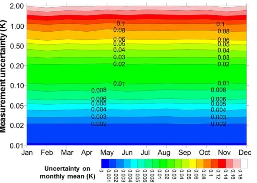
Figure 2 shows the uncertainty on the monthly mean temperature as a function of season and the uncertainty on each individual measurement for 6 hourly sampling throughout the month. There is no contribution to the uncertainty on the monthly mean from sampling because the same 6 hourly sampling is used to derive the “true” monthly mean. Therefore, the uncertainty on the monthly mean is about an order of magnitude

20

smaller than the uncertainty on each instantaneous measurement, which is to be ex-pected when averaging∼120 measurements through the month i.e. 1/√120≈0.1. As can be seen clearly in Fig. 1, the seasonal influence is minimal.

Figure 3 shows the uncertainty on the monthly means for the same location and pres-sure level as in Fig. 2 but now for a range of different sampling strategies, including the

25

(7)

ACPD

15, 1617–1650, 2015

K. Kreher et al.

Title Page

Tables Figures

◭ ◮

Back Close

Full Screen / Esc

Discussion

P

a

per

|

Discussion

P

a

per

|

Discussion

P

a

per

|

Discussion

P

a

per

|

temperatures very different to what would be achieved when sampling every 24 h at midnight, the SD of the differences between the calculated monthly mean and the true monthly mean (rather than the absolute value) is what is assessed. The uncertainty on the monthly mean now shows a clear seasonal cycle for 12 hourly sampling, or coarser, since the temperatures show a higher degree of variability in the winter months at this

5

location and level. At this pressure level (50 hPa), reductions in measurement uncer-tainty below 0.2 K have little effect on the uncertainty on the monthly mean because it is the uncertainty resulting from incomplete sampling that dominates. It is only for a mea-surement uncertainty greater than 0.2 K that the meamea-surement uncertainty begins to make an appreciable contribution to the uncertainty on the monthly mean. This 0.2 K

10

threshold does not only apply to the one location displayed in Fig. 3 but is also valid for the other locations at 50 hPa as well as most other sites at 500 hPa (not shown here). The 0.2 K threshold also supports the GRUAN target of less than 0.2 K uncertainty for instantaneous stratospheric temperature measurements (Immler et al., 2010). The permissible measurement uncertainty varies with pressure and season.

15

The permissible uncertainty of individual temperature measurements required to avoid increasing the uncertainty on the monthly means by more than 10 % above what would be achieved when sampling with 0.01 K uncertainty is shown in Fig. 4. Results from all the 87 locations selected for this analysis and for all months were averaged to produce this figure, with the individual curves showing the permissible uncertainty for

20

each of the 11 sampling schemes.

When sampling every 12 h, at noon/midnight or at 6 a.m./6 p.m. (solid blue and cyan curves), in the upper stratosphere, measuring with 0.5 K uncertainty is su_fficient to avoid affecting the uncertainty of the monthly means by more than 10 %; this reduces to 0.25 K at_∼20 hPa and to 0.15 K in the free troposphere. If the frequency of sampling

25

(8)

ACPD

15, 1617–1650, 2015

K. Kreher et al.

Title Page

Tables Figures

◭ ◮

Back Close

Full Screen / Esc

Discussion

P

a

per

|

Discussion

P

a

per

|

Discussion

P

a

per

|

Discussion

P

a

per

|

or less since this minimizes the uncertainty on the resultant monthly means, thereby allowing for more robust estimates of upper-air temperature trends. For sites sampling only once per week, or less frequently (blue, green and red dashed curves in Fig. 4), a measurement uncertainty of 0.5 K is sufficient to ensure that there is no additional in-crease in the random uncertainty of the resultant monthly means. Of course with such

5

infrequent sampling the monthly means will have greater uncertainties than with more frequent sampling.

2.2 Sampling strategies, measurement uncertainty, and trend detection

The effects of individual measurement uncertainty and sampling strategy on the abil-ity to detect upper air temperature trends has also been investigated using the NCEP

10

CFSR reanalyses temperature profiles. Temperature trends were calculated at each of the 37 pressure levels, for each of the 87 locations using a state-of-the-art regres-sion model (Bodeker et al., 1998). Residuals from the regresregres-sion model fit were then used in a Monte Carlo bootstrap resampling to create 1000 statistically identical time series, each of which was passed through the regression model to create a histogram

15

of trends. Blocks of residuals are selected so as to preserve the autocorrelation struc-ture in the original time series. This method was applied to each of the monthly mean time series, as generated above, based on different assumptions about the uncertainty of each of the individual temperature measurements, and the 12 di_fferent sampling strategies (see Fig. 3 and caption of Fig. 4).

20

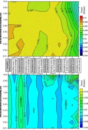
Two examples of the effects of (1) uncertainty on individual measurements and (2) sampling strategy on the quantification of temperature trends are displayed in Fig. 5. The graph shows that at this location and pressure, only sampling less frequently than once weekly, and with measurement uncertainty _≥2 K is the quality of trend detec-tion significantly degraded. At 50 hPa and 39.95◦N, 105.2◦W (lower panel of Fig. 5),

25

(9)

ACPD

15, 1617–1650, 2015

K. Kreher et al.

Title Page

Tables Figures

◭ ◮

Back Close

Full Screen / Esc

Discussion

P

a

per

|

Discussion

P

a

per

|

Discussion

P

a

per

|

Discussion

P

a

per

|

As in the previous example, it is only when the measurement uncertainty exceeds 2 K, and measurements are made only once or twice per month, is the robustness of the trend determination compromised.

3 Site selection for temperature trend detection

In this section, we address the question: which of the existing sites engaged in

upper-5

air temperature measurements are best located to detect expected future trends in upper-air temperatures within the shortest time possible? To do so, we explore and discuss one objective method (without claiming that it is the best or only method) for selecting the optimal locations for detecting projected 21st century temperature trends at approximately 5 and 17.5 km altitude in the shortest time possible.

10

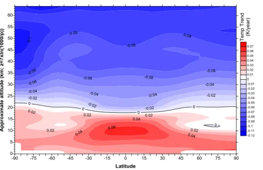
To provide specific guidance based on the material presented in Sect. 2, we investi-gated the number of years it would take to detect projected trends in upper-air temper-atures for specified sampling regimens (both in terms of frequency and measurement uncertainty). Figure 6 shows expected 21st century trends in upper-air temperatures obtained by averaging trends from REF-B2 simulations made by 11 chemistry–climate

15

models as part of the SPARC CCMVal-2 activity (e.g. Young et al., 2013). REF-B2 is the so-called reference simulation and is a self consistent transient simulation from 1960 to 2100 (Eyring et al., 2010). In this simulation the surface time series of halocarbons are based on the adjusted A1 scenario from WMO (2007). The adjusted A1 halogen scenario includes the earlier phase out of hydrochlorofluorocarbons (HCFCs) that was

20

(10)

ACPD

15, 1617–1650, 2015

K. Kreher et al.

Title Page

Tables Figures

◭ ◮

Back Close

Full Screen / Esc

Discussion

P

a

per

|

Discussion

P

a

per

|

Discussion

P

a

per

|

Discussion

P

a

per

|

The number of years of measurements required to detect a trend at the 95 % confi-dence level with a probability of 0.9 can be approximated by (Whiteman et al., 2011):

n∗=





3.3σN

|ω0|

s

1+φN

1₋φ_N 



2/3

(1)

whereσNis the SD of the unforced variability in the time series, i.e. the SD of the

resid-uals after the application of the regression model (described in Sect. 2.2) to remove all

5

known sources of variability,ω0is the trend magnitude in K year− 1

(see Fig. 6), andφ_N

is the autocorrelation in the residuals (Tiao et al., 1990).

This equation implies that after the calculated number of years, there is a 90 % prob-ability that a trend of the correct sign will have been detected, if we assume that detect-ing a trend means identifydetect-ing a trend at the 95 % confidence level.σN and φN values

10

for the 87 analysis locations at the 37 pressure levels were calculated from the NCEP CFSR time series for the 120 different sampling regimens (i.e. 12 sampling strategies for 10 different measurements uncertainties ranging from 0.01–10 K).

When used in Eq. (1) together with the projected 21st century temperature trends shown in Fig. 6, examples of results for two sites are shown in Fig. 7. Calculations

15

were made for 3219 cases (87 locations and 37 pressure levels). Typically, it is only when the uncertainty on each measurement exceeds 2 K, is the ability to detect trends significantly compromised, consistent with the findings presented in Sect. 2.2.

When comparing the results for the two sites displayed in Fig. 7, one in the tropics and one at high latitudes, it is clear that the uncertainty on each temperature

measure-20

ment, has little impact on the time required to detect the projected trend. Similarly, it is only for sampling regimens of every 4 days, or less frequently, that the sampling fre-quency affects the number of years required to detect the projected trend (see also Seidel and Free, 2006). The biggest effect on the time required to detect the pro-jected trend stems from the natural variability (the noise) in the time series, the

auto-25

(11)

ACPD

15, 1617–1650, 2015

K. Kreher et al.

Title Page

Tables Figures

◭ ◮

Back Close

Full Screen / Esc

Discussion

P

a

per

|

Discussion

P

a

per

|

Discussion

P

a

per

|

Discussion

P

a

per

|

25◦N the projected trend is expected to be detected within 30 years or less, for the site at 85◦N, the projected trend will likely not be detected within 100 years.

To further synthesize the results, three pressure levels, viz. 50, 10, and 1 hPa were selected to investigate which measurement regimens, if any, allow for the detection of a temperature trend within 30 years, assuming an uncertainty on each measurement

5

of 1 K. It is apparent from the analysis (not shown here) that in the upper stratosphere (1 hPa), it is possible to detect temperature trends in the tropics (30◦S to 30◦N) with almost any measurement programme – even one measurement per month would be sufficient to detect the trend within 30 years. Over the Arctic however, no measure-ment regimen, no matter how frequently the measuremeasure-ments are made, and even if the

10

measurements are made with very small uncertainty (at 0.01 K), would detect the an-nual temperature trend within 30 years. In contrast to this, in the Antarctic, most mea-surement regimens (at 1 K uncertainty) would detect the trend within 30 years. Over the southern mid-latitudes, the trends would be detected at only one location within 30 years, whereas over northern mid-latitudes, trends may be detected at several

loca-15

tions.

At 10 hPa, the situation is similar to the 1 hPa level, with tropical trends being de-tected more easily than extra-tropical ones, but the robustness now also extends to northern mid-latitudes. The trend detection over the Antarctic is less robust. At 50 hPa, trends may be detectable at up to half of the locations within the tropics, whereas in

20

the extra-tropical regions, no measurement regimen would lead to the detection of the expected temperature trends within 30 years.

This analysis was performed using annually averaged trends and it might well be that trends in some seasons are more likely to be detectable than in the annual mean, either because the trend is steeper in that season, or because the variability in that season is

25

(12)

ACPD

15, 1617–1650, 2015

K. Kreher et al.

Title Page

Tables Figures

◭ ◮

Back Close

Full Screen / Esc

Discussion

P

a

per

|

Discussion

P

a

per

|

Discussion

P

a

per

|

Discussion

P

a

per

|

then be selected based on the magnitude of the expected trend, the natural variability, and the auto-correlation in the data as detailed in Eq. (1).

To identify such preferable sites where temperature trends could be identified sooner than elsewhere, an analysis based on Microwave Sounding Unit (MSU) and Advanced Microwave Sounding Unit (AMSU) temperature measurements, available from remote

5

sensing systems (Mears and Wentz, 2008), was carried out. Figure 8 shows the results of this analysis for the merged MSU channel 2 and AMSU channel 5 temperatures. These are indicative of the middle troposphere with the weighting function peaking at

∼5 km altitude. The SD of the residuals from the application of the regression model to monthly mean temperatures (Fig. 8a) and the first order auto-correlation coefficient

10

(Fig. 8b) are two of the quantities needed to calculate the number of years required to detect a prescribed temperature trend as detailed in Eq. (1).

The month-to-month variability in the data minimizes in the tropics and maximizes over high latitudes, particularly over the Canadian Arctic. This would suggest that the tropics would be ideally suited to long-term temperature trend detection in the middle

15

troposphere. However, as shown in Fig. 8b, the auto-correlation in the temperature time series also maximizes in the tropics. When the SD on the monthly means and the calculated first order auto-correlation are used together with a prescribed trend of 0.5 K decade−1in Eq. (1), the results shown in Fig. 8c are obtained. Large regions of the tropics and sub-tropics have temperature time series that would be amenable to

detec-20

tion of mid-troposphere temperature trends of 0.5 K decade−1 within∼10 years. How-ever, as seen in Fig. 6, temperature trends at 5 km are not everywhere 0.5 K decade−1. If we use the expected temperature trends at 5 km from Fig. 6 in Eq. (1) then the results displayed in Fig. 8d are obtained. This is the optimal figure to use for deciding where to locate measurement sites for detecting trends in mid-tropospheric temperatures.

25

(13)

ACPD

15, 1617–1650, 2015

K. Kreher et al.

Title Page

Tables Figures

◭ ◮

Back Close

Full Screen / Esc

Discussion

P

a

per

|

Discussion

P

a

per

|

Discussion

P

a

per

|

Discussion

P

a

per

|

found to be the GUAN site at Guam. The next site with the next shortest time to detect expected mid-tropospheric temperature trends, which is at least 6000 km from Guam (since it is not necessary to have sites very close together), is the GUAN station on Tromelin Island. We then continue to look through the list of existing measurement sites, ordered by the number of years required to detect trends, selecting sites that are

5

at least 6000 km away from the already selected sites. The resultant distribution of sites is shown in Fig. 8d and also listed in Table 1. Such a selection of sites would provide good global coverage with a preference for sites in regions where the time to detect expected trends in mid-troposphere temperatures is minimal.

Figure 9 shows the results of a similar analysis, but now using merged MSU channel

10

4 and AMSU channel 9 temperatures indicative of the lower stratosphere (weighting functions peaking at_∼17.5 km). The approach described above is used for selecting the optimal measurement sites, now resulting in different sites including one site in the Arctic (Barrow), as well as one Antarctic site (Amundsen–Scott, South Pole), with less emphasis on tropical sites. The sites shown in Fig. 9 are also listed in Table 2.

15

Note that this is just one possible strategy for selecting sites for detecting expected long-term trends in mid-troposphere and lower stratosphere temperatures. Clearly, dif-ferent strategies would result in a different list of ideal sites and strategies need to be tailored to accommodate other factors such as cost, accessibility, measurement ca-pability etc. The purpose of this exercise is to show that generating fields, such as

20

those shown in Figs. 8d and 9d provide one objective method of selecting the optimal location of sites for detecting long-term temperature trends in different regions of the atmosphere within the shortest possible time.

4 Site selection criteria for the detection of ozone trends

As it was done for upper-air temperature trends, we demonstrate a similar technique

25

(14)

ob-ACPD

15, 1617–1650, 2015

K. Kreher et al.

Title Page

Tables Figures

◭ ◮

Back Close

Full Screen / Esc

Discussion

P

a

per

|

Discussion

P

a

per

|

Discussion

P

a

per

|

Discussion

P

a

per

|

tained from 21 CCM simulations of total column ozone changes over the 21st century under the CCMVal2 REF-B2 scenario. Except for one model (CMAM), sea-surface temperatures and sea-ice concentrations are prescribed from coupled ocean model simulations, either from simulations with the ocean coupled to the underlying general circulation model, or from coupled ocean–atmosphere models used in the IPCC 4th

5

assessment report under the same GHG scenario. At each latitude and longitude, the median ozone trend value from the 21 CCM simulations available was extracted and used as the indicative total column ozone trend.

Trends in total column ozone, unlike those in temperature, are not expected to be linear over the coming century over many regions of the globe. It is therefore less

rele-10

vant to consider the time to detect expected 21st century trends in total column ozone as an indicator of where total column ozone observing sites should be located. For example, if in some region of the globe, such as the tropics, where ozone is expected to increase until the middle of the 21st century and then to decrease thereafter, the time to detect the expected trend until 2100 may be significantly longer than the time to

15

detect the trend until 2050. The approach taken is therefore to first conduct an analy-sis, similar to that for temperature, but considering expected trends in ozone from 2010 to 2020 and identifying which set of locations would be best suited for detecting those expected trends. The trend period is then extended by one year to consider trends from 2010 to 2021, and a second set of sites is identified. This is repeated until 2010–2050,

20

thereby creating 31 sets of optimal sites for detecting ozone trends. An example of the outcomes of this analysis for the 2010–2050 analysis is shown in Fig. 10a.

Monthly mean total column ozone data obtained from the Bodeker Scientific total column ozone database1 spanning the period November 1978 to August 2012 were then analysed for their SD and first order auto-correlation, two of the quantities needed

25

to calculate the number of years required to detect a prescribed total column ozone trend. The model used to derive the residuals was similar to that used in Bodeker et al. (2001), which includes terms accounting for the mean annual cycle, the linear

1

(15)

ACPD

15, 1617–1650, 2015

K. Kreher et al.

Title Page

Tables Figures

◭ ◮

Back Close

Full Screen / Esc

Discussion

P

a

per

|

Discussion

P

a

per

|

Discussion

P

a

per

|

Discussion

P

a

per

|

trend, the quasi-biennial oscillation (QBO), the El Niño Southern Oscillation (ENSO), the solar cycle, and the El Chichón and Mt. Pinatubo volcanic eruptions. The resultant SD of the monthly means and the first order auto-correlation coefficient are displayed in Fig. 10b and c. Month-to-month variability in the data minimizes in the tropics and maximizes over high latitudes, particularly over Siberia. This would suggest that the

5

tropics would be ideally suited to long-term total column ozone trend detection. How-ever, as shown in Fig. 10c, the auto-correlation in the total column ozone also maxi-mizes in the tropics. When the SD of the regression model residuals and the first order auto-correlation are used together with the projected trends in total column ozone, the results shown in Fig. 10d are obtained.

10

In analogy to the temperature trends, one objective strategy (but certainly not the only strategy) to use Fig. 10d to determine optimal locations for measurement sites is to select an existing site closest to the minimum value shown in Fig. 10d. In this case only sites from WOUDC, SHADOZ and NDACC networks were considered.

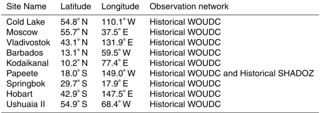
The site closest to the minimum value was found to be the historical WOUDC site at

15

Ushuaia (II). We now look for the next site with the shortest time to detect expected total column ozone trends that is at least 6000 km from Ushuaia. This is found to be Hobart. We then continue to look through the list of existing measurement sites, ordered by the number of years required to detect trends, selecting sites that are at least 6000 km away from sites already selected. The resultant distribution of sites is shown in Fig. 10d

20

and listed in Table 3. Three of the sites in Table 3 are also on the list of the 10 most often selected sites within the 31 sets of optimal sites discussed above and summarized in Table 4. In this analysis, 66 sites were selected in total with 23 of these sites being located in the Southern Hemisphere.

5 Summary

25

(16)

mea-ACPD

15, 1617–1650, 2015

K. Kreher et al.

Title Page

Tables Figures

◭ ◮

Back Close

Full Screen / Esc

Discussion

P

a

per

|

Discussion

P

a

per

|

Discussion

P

a

per

|

Discussion

P

a

per

|

surement uncertainty, sampling frequency, season, and pressure was assessed using NCEP CFSR reanalyses. Our results show that only for individual temperature mea-surement uncertainties greater than 0.2 K, does the meamea-surement uncertainty start to contribute significantly to the uncertainty on the monthly mean. In practical terms, this means that for operational radiosonde stations which carry out temperature profile

5

measurements twice daily, it is worthwhile to work to reduce the uncertainty on each measurement to_≤0.2 K since this minimizes the uncertainty of the resultant monthly means, which should lead to more robust estimates of upper-air temperature trends. However, there is little to be gained by reducing the measurement uncertainty to much less than 0.2 K. This conclusion supports the recommendations made by GRUAN.

10

With a reduction in sampling frequency, the sampling uncertainty starts to dominate, such that less rigorous criteria regarding the uncertainty requirements for each indi-vidual measurement are acceptable. For example, for sites where sampling is only weekly or less frequently, measurement uncertainties of 0.5 K are su_fficient to ensure that there is no additional increase in the random uncertainty on the resultant monthly

15

means by more than 10 % above what would be achieved when sampling with 0.01 K uncertainty. This concurs with the findings of Seidel and Free (2006) who found that if the individual measurement uncertainty is at least 0.5 K, monthly means are accurate to within_∼0.05 K, and SDs are accurate to within 10 %.

Seidel and Free (2006) also found that increasing the uncertainty on temperature

20

measurements has minor effects on the accuracy of the monthly means and SDs and is not an important factor in determining multi-decadal trends. The latter is consistent with our finding that only when the measurement uncertainty exceeds 2 K, and mea-surements are made just once or twice a month or less frequently, the quality of the trend determination is compromised. We find that for a wide range of uncertainties and

25

(17)

ACPD

15, 1617–1650, 2015

K. Kreher et al.

Title Page

Tables Figures

◭ ◮

Back Close

Full Screen / Esc

Discussion

P

a

per

|

Discussion

P

a

per

|

Discussion

P

a

per

|

Discussion

P

a

per

|

30 years or less, while for locations in the northern high latitudes, the projected trend will likely not be detected even within 100 years.

Given these constraints, we have endeavoured to find an objective selection pro-cess for the most suitable measurement sites where temperature trends in the mid-troposphere and lower stratosphere could be identified sooner than elsewhere. Note

5

that this is just one example of an objective site selection strategy and that the resulting maps depend on the criteria used.

A similar technique was applied to find an optimal distribution of measurements sites to detect ozone trends in the shortest time possible. Since trends in total column ozone are not expected to be linear over the coming century over many regions of the globe,

10

it is less pertinent to consider the time to detect expected 21st century trends in total column ozone as an indicator of where total column ozone observing sites should be located. We have therefore investigated different time periods from 2010–2020 up to 2010–2050 to generate 31 sets of optimal sites for ozone trend detection and the 10 measurement sites appearing most often within these 31 sets are listed in Table 4.

15

Studies such as the one presented here provide a sound scientific basis for decision making with regard to new and existing measurements sites and can help reduce costs and concentrate efforts where they are the most needed and most effective.

Acknowledgements. This work was funded in part through the Support to Science Element ESA (European Space Agency) SPARC (Stratosphere–troposphere Processes And their Role

20

in Climate) Initiative (ESA Contract No. 400 010 5291/12/I-NB) and we take this opportunity to acknowledge ESA for this support.

Funding from the NOAA GCOS o_ffice, through the Meteorological Service of New Zealand Ltd, was also essential for completing this work. We would also like to thank Chi-Fan Shih from the National Center for Atmospheric Research in Boulder, CO, for providing the NCEP

25

CFSR reanalyses. We acknowledge the Chemistry–Climate Model Validation (CCMVal) ac-tivity for providing model results from the REF-B2 reference simulations. We also thank the University of Alabama (UAH) and Remote Sensing Systems (RSS) for access to the MSU and AMSU temperature data. The authors wish to thank Anna Mikalsen for helpful comments on the manuscript.

(18)

ACPD

15, 1617–1650, 2015

K. Kreher et al.

Title Page

Tables Figures

◭ ◮

Back Close

Full Screen / Esc

Discussion

P

a

per

|

Discussion

P

a

per

|

Discussion

P

a

per

|

Discussion

P

a

per

|

References

Adams, C., Bourassa, A. E., Sofieva, V., Froidevaux, L., McLinden, C. A., Hubert, D., Lam-bert, J.-C., Sioris, C. E., and Degenstein, D. A.: Assessment of Odin-OSIRIS ozone mea-surements from 2001 to the present using MLS, GOMOS, and ozonesondes, Atmos. Meas. Tech., 7, 49–64, doi:10.5194/amt-7-49-2014, 2014.

5

Balis, D., Kroon, M., Koukouli, M. E., Brinksma, E. J., Labow, G., Veefkind, J. P., and McPeters, R. D.: Validation of Ozone Monitoring Instrument total ozone column measure-ments using Brewer and Dobson spectrophotometer groundbased observations, J. Geophys. Res., 112, D24S46, doi:10.1029/2007JD008796, 2007.

Bodeker, G. E., Boyd, I. S., and Matthews, W. A.: Trends and variability in vertical ozone and

10

temperature profiles measured by ozonesondes at Lauder, New Zealand: 1986–1996, J. Geophys. Res., 103, 28661–28681, 1998.

Bodeker, G. E., Scott, J. C., Kreher, K., and McKenzie, R. L.: Global ozone trends in potential vorticity coordinates using TOMS and GOME intercompared against the Dobson network: 1978–1998, J. Geophys. Res., 106, 23029–23042, 2001.

15

Eyring, V., Cionni, I., Bodeker, G. E., Charlton-Perez, A. J., Kinnison, D. E., Scinocca, J. F., Waugh, D. W., Akiyoshi, H., Bekki, S., Chipperfield, M. P., Dameris, M., Dhomse, S., Frith, S. M., Garny, H., Gettelman, A., Kubin, A., Langematz, U., Mancini, E., Marchand, M., Nakamura, T., Oman, L. D., Pawson, S., Pitari, G., Plummer, D. A., Rozanov, E., Shep-herd, T. G., Shibata, K., Tian, W., Braesicke, P., Hardiman, S. C., Lamarque, J. F.,

Mor-20

genstern, O., Pyle, J. A., Smale, D., and Yamashita, Y.: Multi-model assessment of strato-spheric ozone return dates and ozone recovery in CCMVal-2 models, Atmos. Chem. Phys., 10, 9451–9472, doi:10.5194/acp-10-9451-2010, 2010.

Free, M., Durre, I., Aguilar, E., Seidel, D., Peterson, T. C., Eskridge, R. E., Luers, J. K., Parker, D., Gordon, M., Lanzante, J., Klein, S., Christy, J., Schroeder, S., Soden, B.,

Mcmil-25

lan, L. M., and Weatherhead, E.: Creating climate reference datasets; CARDS Workshop on Adjusting Radiosonde Temperature Data for Climate Monitoring, B. Am. Meteorol. Soc., 83, 891–899, 2002.

Immler, F. J., Dykema, J., Gardiner, T., Whiteman, D. N., Thorne, P. W., and Vömel, H.: Ref-erence Quality Upper-Air Measurements: guidance for developing GRUAN data products,

30

(19)

ACPD

15, 1617–1650, 2015

K. Kreher et al.

Title Page

Tables Figures

◭ ◮

Back Close

Full Screen / Esc

Discussion

P

a

per

|

Discussion

P

a

per

|

Discussion

P

a

per

|

Discussion

P

a

per

|

IPCC (Intergovernmental Panel on Climate Change): Special Report on Emissions Scenarios: a Special Report of Working Group III of the Intergovernmental Panel on Climate Change, Cambridge University Press, Cambridge, UK, 599 pp., 2000.

Mears, C. A. and Wentz, F. J.: Construction of the Remote Sensing Systems V3.2 Atmospheric Temperature Records from the MSU and AMSU Microwave Sounders, J. Atmos. Ocean.

5

Tech., 26, 1040–1056, 2008.

Saha, S., Moorthi, S., Pan, H.-L., Wu, X., Wang, J., Nadiga, S., Tripp, P., Kistler, R., Woollen, J., Behringer, D., Liu, H., Stokes, D., Grumbine, R., Gayno, G., Wang, J., Hou, Y.-T., Chuang, H.-Y., Juang, H.-M. H., Sela, J., Iredell, M., Treadon, R., Kleist, D., Van Delst, P., Keyser, D., Derber, J., Ek, M., Meng, J., Wei, H., Yang, R., Lord, S., van den Dool, H., Kumar, A., Wang,

10

W., Long, C., Chelliah, M., Xue, Y., Huang, B., Schemm, J.-K., Ebisuzaki, W., Lin, R., Xie, P., Chen, M., Zhou, S., Higgins, W., Zou, C.-Z., Liu, Q., Chen, Y., Han, Y., Cucurull, L., Reynolds, R. W., Rutledge, G., and Goldberg, M.: The NCEP climate forecast system reanalysis, B. Am. Meteorol. Soc., 91, 1015–1057, 2010.

Seidel, D. J. and Free, M.: Measurement requirements for climate monitoring of upper-air

tem-15

perature derived from reanalysis data, J. Climate, 19, 854–871, 2006.

Thompson, D. W. J., Seidel, D. J., Randel, W. J., Zou, C., Butler, A. H., Mears, C., Osso, A., Long, C., and Lin, R.: The mystery of recent stratospheric temperature trends, Nature, 491, 692–697, 2012.

Tiao, G. C., Reinsel, G. C., Xu, D., Pedrick, J. H., Zhu, X., Miller, A. J., DeLuisi, J. J.,

Ma-20

teer, C. L., and Wuebbles, D. J.: Effects of autocorrelation and temporal sampling schemes on estimates of trend and spatial correlation, J. Geophys. Res., 95, 20507–20517, 1990. Tobin, D. C., Revercomb, H. E., Knuteson, R. O., Lesht, B. M., Strow, L. L., Hannon, S. E.,

Feltz, W. F., Moy, L. A., Fetzer, E. J., and Cress, T. S.: Atmospheric radiation measurement site atmospheric state best estimates for atmospheric infrared sounder temperature and

wa-25

ter vapor retrieval validation, J. Geophys. Res., 111, D09S14, doi:10.1029/2005JD006103, 2006.

Tummon, F., Hassler, B., Harris, N. R. P., Staehelin, J., Steinbrecht, W., Anderson, J., Bodeker, G. E., Bourassa, A., Davis, S. M., Degenstein, D., Frith, S. M., Froidevaux, L., Kyrölä, E., Laine, M., Long, C., Penckwitt, A. A., Sioris, C. E., Rosenlof, K. H., Roth, C.,

30

(20)

ACPD

15, 1617–1650, 2015

K. Kreher et al.

Title Page

Tables Figures

◭ ◮

Back Close

Full Screen / Esc

Discussion

P

a

per

|

Discussion

P

a

per

|

Discussion

P

a

per

|

Discussion

P

a

per

|

Wang, J. S., Seidel, D. J., and Free, M.: How well do we know recent climate trends at the tropical tropopause?, J. Geophys. Res., 117, D09118, doi:10.1029/2012JD017444, 2012. Whiteman, D. N., Vermeesch, K. C., Oman, L. D., and Weatherhead, E. C.: The relative

impor-tance of random error and observation frequency in detecting trends in upper tropospheric water vapor, J. Geophys. Res., 116, D21118, doi:10.1029/2011JD016610, 2011.

5

World Meteorological Organization (WMO)/United Nations Environment Programme (UNEP), Scientific Assessment of Ozone Depletion: 2006, Global Ozone Research and Monitoring Project, Report No. 50, Geneva, Switzerland, 572 pp., 2007.

Young, P. J., Butler, A. H., Calvo, N., Haimberger, L., Kushner, P. J., Marsh, D. R., Randel, W. J., and Rosenlof, K. H.: Agreement in late twentieth century Southern Hemisphere stratospheric

10

(21)

ACPD

15, 1617–1650, 2015

K. Kreher et al.

Title Page

Tables Figures

◭ ◮

Back Close

Full Screen / Esc

Discussion

P

a

per

|

Discussion

P

a

per

|

Discussion

P

a

per

|

Discussion

P

a

per

|

Table 1.Proposed measurement sites for the detection of 21st century temperature trends at the middle troposphere.

Site Name Latitude Longitude Observation network Annette Island 55.0◦N 131.3◦E GUAN

La Coruna 43.3◦N 8.5◦W GUAN, WOUDC Kashi 39.3◦N 75.6◦E GUAN

Kingston 17.6◦N 76.5◦W GUAN Guam 13.3◦N 144.5◦E GUAN Tromelin Island 15.5◦S 54.3◦E GUAN St. Helena 15.6◦S 5.4◦W GUAN Rarotonga 21.1◦S 159.5◦W GUAN Puerto Montt 41.3◦S 73.1◦W GUAN

(22)

ACPD

15, 1617–1650, 2015

K. Kreher et al.

Title Page

Tables Figures

◭ ◮

Back Close

Full Screen / Esc

Discussion

P

a

per

|

Discussion

P

a

per

|

Discussion

P

a

per

|

Discussion

P

a

per

|

Table 2.Proposed measurement sites for the detection of 21st century temperature trends at the lower stratosphere.

Site Name Latitude Longitude Observation network Barrow 71.3◦N 156.6◦W GRUAN, ARM, GAW Key West 24.3◦N 81.5◦W GUAN

Asswan 23.6◦N 32.5◦E GUAN Chichijima 27.1◦N 142.1◦E GUAN Rapa 27.4◦S 144.2◦W GUAN Perth Airport 31.6◦S 115.6◦E GUAN Cape Town 33.6◦S 18.4◦E GUAN Ezeiza Aero 34.5◦S 58.3◦W GUAN

(23)

ACPD

15, 1617–1650, 2015

K. Kreher et al.

Title Page

Tables Figures

◭ ◮

Back Close

Full Screen / Esc

Discussion

P

a

per

|

Discussion

P

a

per

|

Discussion

P

a

per

|

Discussion

P

a

per

|

Table 3.Proposed measurement sites for the detection of ozone trends from 2010–2050.

Site Name Latitude Longitude Observation network Cold Lake 54.8◦N 110.1◦W Historical WOUDC Moscow 55.7◦N 37.5◦E Historical WOUDC Vladivostok 43.1◦N 131.9◦E Historical WOUDC Barbados 13.1◦N 59.5◦W Historical WOUDC Kodaikanal 10.2◦N 77.4◦E Historical WOUDC

Papeete 18.0◦S 149.0◦W Historical WOUDC and Historical SHADOZ Springbok 29.7◦S 17.9◦E Historical WOUDC

(24)

ACPD

15, 1617–1650, 2015

K. Kreher et al.

Title Page

Tables Figures

◭ ◮

Back Close

Full Screen / Esc

Discussion

P

a

per

|

Discussion

P

a

per

|

Discussion

P

a

per

|

Discussion

P

a

per

|

Table 4.The five most frequently selected Northern Hemisphere sites in the 31 sets of optimal sites followed by the five most frequently selected Southern Hemisphere sites.

Site Name Latitude Longitude Observation network Kyiv-Goloseyev 50.3◦N 30.5◦E Current WOUDC Sapporo 43.0◦N 141.3◦E Current WOUDC, GUAN Moscow 55.7◦N 37.5◦E Historical WOUDC Edmonton/Stony Pl. 53.5◦N 114.1◦W Historical WOUDC Coolidge Field 17.3◦N 61.8◦W Historical WOUDC Hobart 42.9◦S 147.5◦E Historical WOUDC

Papeete 18.0◦S 149.0◦W Historical WOUDC and Historical SHADOZ La Reunion Island 21.1◦S 55.5◦E Historical WOUDC

Ushuaia 54.9◦S 68.3◦W Current WOUDC, GAW

(25)

ACPD

15, 1617–1650, 2015

K. Kreher et al.

Title Page

Tables Figures

◭ ◮

Back Close

Full Screen / Esc

Discussion

P

a

per

|

Discussion

P

a

per

|

Discussion

P

a

per

|

Discussion

P

a

per

|

(26)

ACPD

15, 1617–1650, 2015

K. Kreher et al.

Title Page

Tables Figures

◭ ◮

Back Close

Full Screen / Esc

Discussion

P

a

per

|

Discussion

P

a

per

|

Discussion

P

a

per

|

Discussion

P

a

per

|

(27)

ACPD

15, 1617–1650, 2015

K. Kreher et al.

Title Page

Tables Figures

◭ ◮

Back Close

Full Screen / Esc

Discussion

P

a

per

|

Discussion

P

a

per

|

Discussion

P

a

per

|

Discussion

P

a

per

|

(28)

ACPD

15, 1617–1650, 2015

K. Kreher et al.

Title Page

Tables Figures

◭ ◮

Back Close

Full Screen / Esc

Discussion

P

a

per

|

Discussion

P

a

per

|

Discussion

P

a

per

|

Discussion

P

a

per

|

(29)

ACPD

15, 1617–1650, 2015

K. Kreher et al.

Title Page

Tables Figures

◭ ◮

Back Close

Full Screen / Esc

Discussion

P

a

per

|

Discussion

P

a

per

|

Discussion

P

a

per

|

Discussion

P

a

per

|

(30)

ACPD

15, 1617–1650, 2015

K. Kreher et al.

Title Page

Tables Figures

◭ ◮

Back Close

Full Screen / Esc

Discussion

P

a

per

|

Discussion

P

a

per

|

Discussion

P

a

per

|

Discussion

P

a

per

|

(31)

ACPD

15, 1617–1650, 2015

K. Kreher et al.

Title Page

Tables Figures

◭ ◮

Back Close

Full Screen / Esc

Discussion

P

a

per

|

Discussion

P

a

per

|

Discussion

P

a

per

|

Discussion

P

a

per

|

(32)

ACPD

15, 1617–1650, 2015

K. Kreher et al.

Title Page

Tables Figures

◭ ◮

Back Close

Full Screen / Esc

Discussion

P

a

per

|

Discussion

P

a

per

|

Discussion

P

a

per

|

Discussion

P

a

per

|

(33)

ACPD

15, 1617–1650, 2015

K. Kreher et al.

Title Page

Tables Figures

◭ ◮

Back Close

Full Screen / Esc

Discussion

P

a

per

|

Discussion

P

a

per

|

Discussion

P

a

per

|

Discussion

P

a

per

|

Figure 9.Analyses of merged MSU channel 4 and AMSU channel 9 temperature data – 1978 to 2013.(a) SD of regression model residuals, (b)the first order auto-correlation coefficient of the residuals,(c)the number of years required to detect a trend of 0.5 K decade−1, and(d)

(34)

ACPD

15, 1617–1650, 2015

K. Kreher et al.

Title Page

Tables Figures

◭ ◮

Back Close

Full Screen / Esc

Discussion

P

a

per

|

Discussion

P

a

per

|

Discussion

P

a

per

|

Discussion

P

a

per

|