Numerical and experimental analysis of yield loads in welded gap hollow YT-joint

(1)

Numerical and experimental analysis of yield loads in welded

gap hollow YT-joint

Abstract

This paper presents an analytical, experimental, and numer-ical analysis of plain steel, circular hollow sections welded into a YT joint. The overall behavior and failure of the joint are characterized under axial compression of the lap brace. There are two joint failure modes: plastic failure of the chord face and local buckling of the chord walls. Numerical finite element models agree with the experimental data, in terms of principal stress near the joint intersection, with an accuracy of around 10%. The finite element model thus proves to be reliable and accurate, and will be used in future parametric studies.

Keywords

Hollow structures, joints, numerical analysis, experimental analysis.

R. F. Vieiraa,∗, J. A. V.

Requenaa, A. M. S. Freitasband V. F. Arcaroa

a_{State University of Campinas, Campinas, SP}

– Brazil

b_{Federal University of Ouro Preto, Ouro Preto,}

MG – Brazil

Received 6 May 2009; In revised form 1 Oct 2009

∗_{Author email: [email protected]}

1 INTRODUCTION

One of the reasons that steel structures are used more frequently in buildings nowadays is that their manufacturing process presents several economic advantages. In this context, the increasing demand for hollow sections worldwide must be pointed out; they have provided many buildings with an elegant and modern look. Thus, one of the factors that determine the cost of steel structures is the manufacturing of standardized hollow sections.

The most common hollow sections have square (SHS-Square Hollow Sections), rectangular (RHS-Rectangular Hollow Sections), or circular cross sections (CHS-Circular Hollow Sections). They are made of highly resistant steel, the yield stress is around 350MPa. One of the compa-nies that manufacture this material in Brazil is VALLOUREC & MANNESMANN TUBES, or V&M do BRASIL S.A. (formerly Mannesmann S.A.). It was founded in 1953 at the request of the Brazilian government, to meet the growing demand of their oil industry.

(2)

364 R.F. Vieira et al / Numerical and experimental analysis of yield loads in welded gap hollow YT-joint

NOMENCLATURE

Ai cross sectional area of member i(i=0,1,2,3)

E modulus of elasticity

Et modulus of elasticity tangent

M0 bending moment in the chord member

Ni axial force applied to memberi (i=0,1,2,3)

N_i∗ joint design resistance expressed in terms of axial load in member i N0_P pre-stressing axial force on the chord

W0 elastic section modulus of member i(i=0,1,2,3)

di external diameter of circular hollow section for member i(i=0,1,2,3)

e nodding eccentricity for a connection

fy yield stress

fyi yield stress of member i(i=0,1,2,3)

f0P pre-stress in chord

f(n) function which incorporates the chord pre-stress in the joint resistance equation

g gap between the bracings members of a K, N or KT joint, at the face of the chord

g′ gap divided by chord wall thickness

n′ f0P fy0

= N0P A0⋅fy0+

M0 W0⋅fy0

t_i thickness of hollow section member i(i=0,1,2,3)

β diameter ratio between bracing on chord

β= d1 d0,

d1 b0,

bi

b0 T, Y andX

β= d1+d2

2_⋅d0 , d1+d2

2_⋅b0 ,

b1+b2+h1+h2

4_⋅b0 KandN

γ ratio of the chord’s half diameter to its thickness

ν poisson’s ratio

θ included angle between bracing member i(i=0,1,2,3) and the chord

ϵ maximum specific proportionality strain

f stress

flp maximum proportionality stress

fr maximum resistance stress

f1 principal stress 1

f2 principal stress 2

The third stage of this study uses Ansys [2] to model the hollow joints as an assembly of SHELL elements. The experimental results were used to calibrate the numerical model.

2 FAILURE MODES JOINTS

(3)

and Handerson [6] presents the failure modes of bracing K-joints in square and rectangular hollow sections. They are: MODE A – plastic failure of the chord face; MODE B – punching shear failure of the chord face; MODE C – tension failure of the web member; MODE D – local buckling of the web member; MODE E – overall shear failure of the chord; MODE F – local buckling of the chord walls; and MODE G – local buckling of the chord face.

3 CALCULATION OF CONNECTION RESISTANCE

The YT joint prototype design uses the methodology presented by Wardenier et al. (CIDECT 1991) [8] and Packer and Henderson [6].

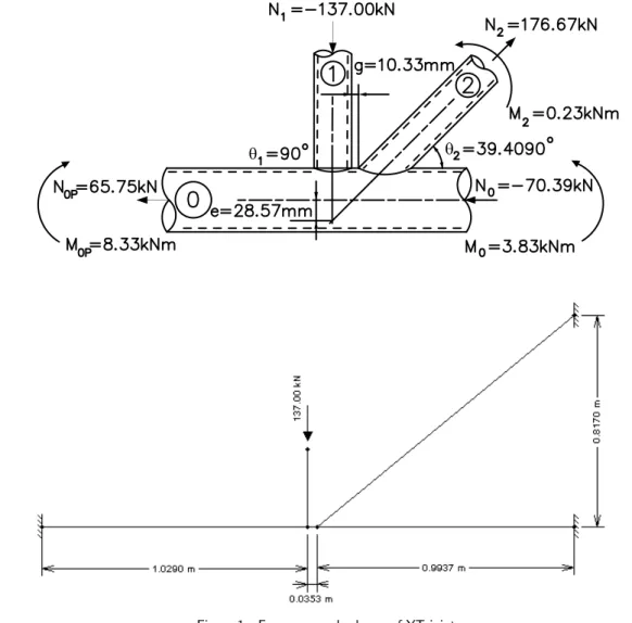
The Fig. 1 shows forces general scheme using as a limit the maximum capacity of the vertical brace member of the YT joint and the bending moment due the eccentricity was not considered.

(4)

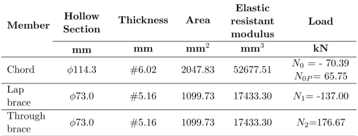
Table 1 shows the geometric characteristics of the VMB 250 circular hollow sections used in the YT joint. The nominal physical proprieties yield stress (fy) are equal 250 MPa.

Table 1 Physical and geometrical characteristics.

Member _SectionHollow Thickness Area

Elastic resistant modulus

Load

mm mm mm2

mm3

kN

Chord ϕ114.3 #6.02 2047.83 52677.51 N0= - 70.39

N0_P= 65.75

Lap

brace ϕ73.0 #5.16 1099.73 17433.30 N1= -137.00

Through

brace ϕ73.0 #5.16 1099.73 17433.30 N2=176.67

3.1 Validity limits

The YT joint meets all geometrical requirements described in the aforementioned references.

3.2 Calculations

a) YT joint parameters

The YT joint parameters are given by Eq. (1) through Eq. (5):

β= d1+d2 2⋅d0

; (1)

g′= g

t0

; (2)

The stress on the chord, f0_P, depends most critically on the compressing stress.

n′= f0P

fy0

= N0P

A0⋅f_y0+

M0

W0⋅f_y0

; (3)

f(n′)=1_.0+0_.3⋅_n′ − 0_.3⋅_n′2 ≤ 1 ; (4)

f(γ, g′)=γ0.2⋅ (1+ 0.024⋅γ

1_.2

1+exp(0_.5_⋅g′₋1_.33₎); (5)

(5)

N1∗=

fy0⋅t 2 0

senθ1 (

1.8+10.2⋅d1

d0) ⋅

f (γ, g′) ⋅ f (n′); (6)

Diagonal through brace:

N2∗=N1∗ ⋅ (

senθ1

senθ2)

; (7)

c) Punching shear failure of the chord face (Mode B)

Vertical lap brace and diagonal through brace are both given by Eq. (8):

N_i∗= fy0⋅t√0⋅π⋅di

3 ⋅ (

1+senθi 2⋅sen2_θ

i)

; (8)

d) YT Joint Resistance

The joint resistance is the lowest value obtained in items (b) and (c) above. Vertical lap brace:

N1

N∗

1

<1; (9)

Diagonal through brace:

N2

N2∗

<1; (10)

Table 2 presents the results of the calculation.

Table 2 Results of the calculation procedure.

Joint parameters Acronym Calculation

Relation between diameters β 0.64

Relation between diameter and thickness γ 9.49

n′=stress/fy (compression) n′ -0.14

Function of prestress on chord f(n′₎ _0.95

Resistance plastic failure of the chord face (Mode A) N∗

1(Pl) 137.40 kN

Resistance punching shear failure of the chord face (Mode B) N∗

1(Pu) 199.27 kN

Lap brace use N1/N1∗ 1.0

Resistance plastic failure of the chord face (Mode A) N2∗(Pl) 216.42 kN

Resistance punching shear failure of the chord face (Mode B) N2∗(Pu) 404.16 kN

(6)

4 EXPERIMENTAL PROGRAM

To study the joint, it was first necessary to determine the mechanical properties of the material through test-body traction. Then four prototypes constructed from seamless rolled tubes were manufactured by V&M do Brasil. They were called pre-experiment, experiments I, II and III.

4.1 Traction test

A stress-strain diagram was obtained through test-body traction measurements [1].

Table 3 presents data obtained from the stress-strain diagram. The flp term is defined as the stress that corresponds to a strain of approximately 0.0012 [5].

Table 3 Data provided by the stress-strain diagram.

Test Bodies ϵ flp fy fr E

X10-6 MPa MPa MPa MPa

cp1a - ϕ73mm 1199 259.3 314.5 480.3 216222.8

cp1b -ϕ73mm 1165 220.3 326.0 486.9 189114.6

cp2a - ϕ114.3mm 1062 323.2 332.2 465.1 304461.5

cp2b -ϕ114.3mm 1165 264.9 322.6 473.6 227390.8

4.2 YT joint prototypes

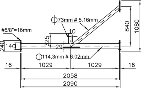
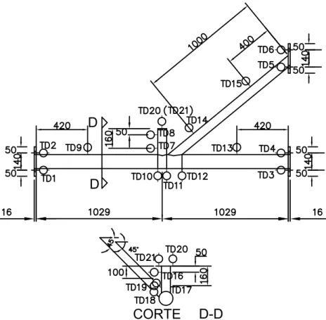
The dimensions of the prototypes are shown in Fig. 2. The prototypes are fixed by four screws at each end. They were loaded axially at the top of the lap brace.

(7)

4.3 Instrumentation for tests

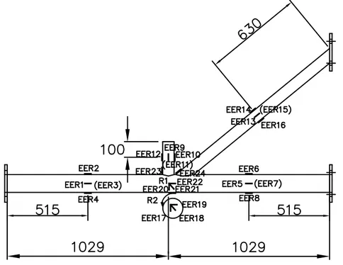
In EXPERIMENTS I, II and III, sixteen 5mm electrical resistance KFG-5-120-C1-11 exten-someters were used. Their positions are marked EER1 to EER16 in Fig. 3.

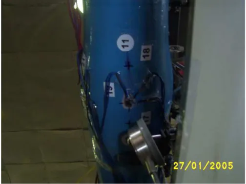
The EERs were placed on the prototype to measure longitudinal strain, drawing on the work of FUNG et al [4]. In EXPERIMENT III, 2 rosette gauges and 2 individual extensometers were added (for a total of 24 EERs). Rosette 1 was composed of EER20, EER21 and EER22; rosette 2 was composed of EER17, EER18 and EER19. EER23 and EER24 were placed at the bases of the lap brace and through brace respectively.

Figure 3 Positioning of the extensometers on the YT joint prototype.

In EXPERIMENTS I, II and III, 19 manual reading displacement transducers (TD1 to TD19) and two digital reading displacement transducers (TD20 and TD21) were placed on the prototype as shown in Fig. 4.

4.4 Experimental results

The testing methodology used was defined in three stages, as shown below:

(8)

Figure 4 Positioning of the DTs on the YT joint prototype.

• Stage II - During the test the speed of the actuator load was kept as slow and steady as possible for both the case of loading and for unloading. The step load was previously set depending on the stage supposed to loading. At each step of loading, when the pre established loading was reached, expected time to stabilize the transducers and then did the reading.

• Stage III- The prototype was loaded to the ultimate state, where the prototype did not offer more resistance, even after he reached the break. Then the prototype was unloaded.

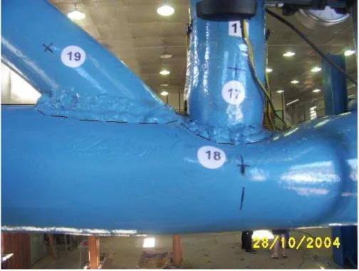
Fig. 5 shows the overall strain of the prototype in EXPERIMENT III, characterized by the development of failure Mode A.

(9)

Figure 5 Overall strain of the prototype for EXPERIMENT III.

(10)

Figure 7 Failure Mode F: local buckling of the chord face.

The results of the last loading for each of the tests are shown in Table 4.

Table 4 Last loading to EXPERIMENTS I, II and III.

EXPERIMENTS Last loading (kN)

EXPERIMENT I 240,0

EXPERIMENT II 358,6

EXPERIMENT III 316,4

Two failure modes were observed: plastic failure of the chord face (Mode A) and local buckling of the chord walls (Mode F).

4.5 Presentation and analysis of the test results

(11)

5 ANALYSIS OF FINITE ELEMENTS

Two numerical models were created in Ansys, one using a bilinear stress-strain diagram (BISO – Bilinear Isotropic Hardening) and the other a multilinear (piecewise linear) diagram (MISO – Multilinear Isotropic Hardening). Their results were compared to the experimental tests.

Both physical and geometrical non-linearity were considered in the analysis. To implement physical non-linearity, we used the stress-strain diagrams obtained in our traction test of the prototype (Section 4.1).

The contour conditions were simulated in Ansys through displacement restrictions. Force was applied in an increasing way, that is, at unit load pitches.

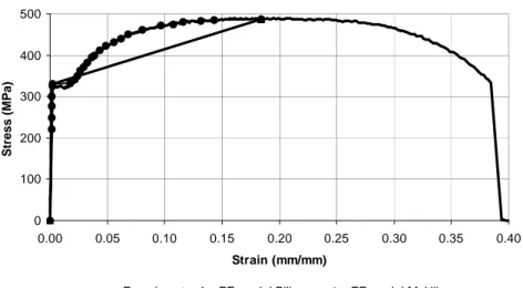
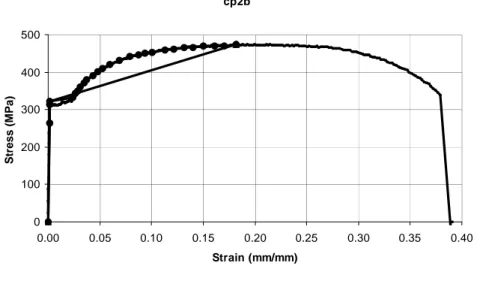
Fig. 8 and Fig. 9 show the stress-strain diagrams of test bodies selected for the numerical analysis. The multilinear model is represented by 26 points (crossed circles), and the bilinear model by two straight lines (triangles).

cp1b

0 100 200 300 400 500

0.00 0.05 0.10 0.15 0.20 0.25 0.30 0.35 0.40

Strain (mm/mm)

S

tr

e

s

(

M

P

a

)

Experiment FE model Bilinear FE model Multilinear

Figure 8 Experimental, bilinear and multilinear stress-strain diagrams used for test body cp1b, from the through brace and lap brace (φ73mm).

Table 5 shows data used to represent the material properties of test bodies cp1b and cp2b in the numerical model. Note that the bilinear stress-strain diagram always runs from the origin to the first stress peak (f), then from this point to the maximum stress (fr) of the material.

Table 5 Data used to represent the bilinear stress-strain diagram with the Ansys software (BISO).

Test Body fy f fr E Et

MPa MPa MPa MPa MPa

cp1b(ϕ73mm) 326.0 331.1 486.9 189114.6 856.5

(12)

cp2b

0 100 200 300 400 500

0.00 0.05 0.10 0.15 0.20 0.25 0.30 0.35 0.40

Strain (mm/mm)

S

tr

e

s

(

M

P

a

)

Experiment FE model Bilinear FE model Multilinear

Figure 9 Experimental, bilinear and multilinear stress-strain diagrams used for test body cp2b, from the chord (φ114,3mm).

The 26 points to represent the multilinear stress-strain diagram is shown by Table 6.

Table 6 Data used to represent the multilinear stress-strain diagram with the Ansys software (MISO).

cp1b(ϕ73mm) cp2b(ϕ114,3mm)

Points e f E e f E

Dimensionless GPa GPa Dimensionless GPa GPa

0 0 0 0 0 0 0

1 0.001165 0.22031 189.1146 0.001165 0.2649 227.3908

2 0.0013373 0.24958 186.6298 0.0014234 0.31285 219.7906

3 0.0015613 0.27689 177.3458 0.0017508 0.32257 184.2415

4 0.0017853 0.29975 167.899 0.023651 0.33273 14.06833

5 0.001992 0.32604 163.6747 0.026081 0.34245 13.13025

6 0.0022849 0.3311 144.9079 0.028562 0.3501 12.25754

7 0.017672 0.3324 18.80942 0.031181 0.3607 11.56794

8 0.021394 0.34219 15.99467 0.034834 0.37027 10.62956

9 0.023668 0.35058 14.8124 0.037418 0.38073 10.17505

10 0.026442 0.36218 13.69715 0.043173 0.39133 9.06423

11 0.029286 0.3713 12.67841 0.047722 0.40085 8.39969

12 0.032646 0.38115 11.67524 0.052478 0.41042 7.820801

13 0.036229 0.39585 10.92633 0.059905 0.42068 7.022452

(13)

Table 6 Data used to represent the multilinear stress-strain diagram with the Ansys software (MISO) (contin-uation).

cp1b(ϕ73mm) cp2b(ϕ114,3mm)

Points e f E e f E

Dimensionless GPa GPa Dimensionless GPa GPa

14 0.038728 0.40007 10.33025 0.068554 0.43103 6.287452

15 0.043656 0.41183 9.433526 0.0786 0.44115 5.612595

16 0.048567 0.42287 8.706941 0.0874737 0.44546 5.092552

17 0.055838 0.43131 7.72431 0.093987 0.45077 4.796089

18 0.061989 0.44038 7.104164 0.1006035 0.45302 4.50305

19 0.068227 0.4504 6.601492 0.11285 0.46019 4.077891

20 0.080736 0.46188 5.720868 0.12118 0.46171 3.810117

21 0.096589 0.47179 4.884511 0.13124 0.465 3.543127

22 0.1074614 0.47472 4.417572 0.14001 0.46647 3.331691

23 0.1159 0.48035 4.144521 0.15042 0.46932 3.120064

24 0.1316533 0.48221 3.662694 0.1611 0.4701 2.918063

25 0.14347 0.48564 3.384959 0.17035 0.47025 2.760493

26 0.18417 0.48688 2.643644 0.18148 0.47364 2.609874

The Poisson’s ratio was obtained by compression test tube used. The value obtained was

ν=0.3.

The SHELL element was considered most appropriate to represent hollow structures. Specifically, the SHELL181 element was used to generate a mesh for the hollow sections. The SHELL63 element was used for fixation plates. Table 7 shows their characteristics.

Table 7 Characteristics of elements.

Elements Nr of nodes

per element

Degrees of

freedom Special features

SHELL 63 4 6 Elastic Large

deflection

Little strain

SHELL 181 4 6 Plastic Large

deflection

Large strain

(14)

Figure 10 Finite element model of the YT joint prototype.

Figure 11 Principal stress (f1) for the multilinear model (GPa).

6 COMPARISON BETWEEN EXPERIMENTAL TEST RESULTS AND NUMERICAL

MODEL RESULTS

The experimental tests and numerical models can be compared on the basis of strains obtained by the extensometers.

In EXPERIMENT II several loading and unloading cycles were carried out, with slight strain occurring in each cycle. In this case, we only report the results of the last cycle. This is why the readings reported for EXPERIMENT II do not present zero initial strain.

(15)

Figure 12 Detail of the multilinear model strain.

The strain on the chord was recorded by extensometers EER1 to EER8. These points do not represent plastic strain. In this paper, only the results from extensometers EER1, EER2 and EER4 are presented (Fig. 13, Fig. 14 and Fig. 15 respectively).

EER 1

0 50 100 150 200 250 300

0 50 100 150 200

Strain (x10-6)

A

p

li

e

d

l

o

a

d

(

k

N

)

Experiment I Experiment II Experiment III

FE model Bilinear FE model Multilinear

Figure 13 Chord strain recorded by extensometer EER1 and the numerical models.

The inversion of strain in Fig. 14 indicates the mechanism of failure Mode A.

(16)

378 R.F. Vieira et al / Numerical and experimental analysis of yield loads in welded gap hollow YT-joint EER 2 0 50 100 150 200 250 300

-350 -300 -250 -200 -150 -100 -50 0 Strain (x10-6) A p p li e d l o a d ( k N )

Figure 14 Chord strain recorded by extensometer EER2 and the numerical models.

EER 4 0 50 100 150 200 250 300

0 100 200 300 400 500 600 700 800

Strain (x10-6) A p p li e d l o a d ( k N )

(17)

EER 9 0.0 50.0 100.0 150.0 200.0 250.0 300.0

-1500 -1200 -900 -600 -300 0

Figure 16 Lap brace strain recorded by extensometer EER9 and the numerical models.

For the through brace, only the result from EER13 is shown (Fig. 17).

EER 13 0 50 100 150 200 250 300

0 2000 4000 6000 8000 10000 12000 14000

Figure 17 Through brace strain recorded by extensometer EER13 and the numerical models.

(18)

380 R.F. Vieira et al / Numerical and experimental analysis of yield loads in welded gap hollow YT-joint 0 50 100 150 200 250 300

0.00 0.20 0.40 0.60 0.80 1.00 1.20

Displacement (mm) A p p li e d l o a d ( k N )

Experiment I Experiment II FE model Multilinear

Figure 18 Local buckling of the chord face.

As for the rosettes, comparisons between theory and experiment can be made between the principal stresses.

Fig. 19 and Fig. 20 show the principal stresses f1 and f2 measured at rosette 1 in

EX-PERIMENT III and the numerical models.

Rosette 1 0 50 100 150 200 250 300 350 400

0.0 50.0 100.0 150.0 200.0 250.0

Applied load (KN)

P ri n c ip a l s tr e s s 1 ( M P a )

Experiment III FE model Bilinear FE model Multilinear

Figure 19 Principal stressf1measured at rosette 1 in EXPERIMENT III and the numerical models.

The principal stresses f1and f2of the two numerical models were in good agreement with

(19)

Rosette 1 0 50 100 150 200 250

0.0 50.0 100.0 150.0 200.0 250.0

Applied load (KN)

P ri n c ip a l s tr e s s 2 ( M P a )

Experiment III FE model Bilinear FE model Multilinear

Figure 20 Principal stressf2 measured at rosette 1 in EXPERIMENT III and the numerical models.

7 CONCLUSION

The experimental tests and numerical analysis agree that the most critical region of the joint is its intersection, where the greatest stress concentration is found. At this spot there was plasticization.

For each of the hollow sections, the yield stress fy can be obtained by finding the average of the stresses provided during the traction test. The average yield stress of the chord is 330 MPa.

The yield load of the YT joint is whatever load induces the yield stress in at least one section.

The yield load measured by rosette 1 in EXPERIMENT III may not be the yield load of the YT joint, however, because the yield may have occurred at some other point. Still, it must be very close as numerical models identify this area as having the greatest stress concentration. With numerical modeling, it is possible to obtain the yield load at the location correspond-ing to rosette 1. It also provides the real yield load of the finite element model, which can be compared to the yield load of the real YT joint. Table 8 shows the relative error between the principal stresses f1 obtained by numerical models and rosette 1 in EXPERIMENT III. The error is only around 10%, which is quite good.

In the numerical models, the yield load was found by examining all nodes in the chord area corresponding to rosette 1. We took the load on whichever node reached the yield stress (fy=330 MPa) first. The results are shown in Table 9.

(20)

Table 8 Error percentage of the principal stress, f1, for the spot represented by rosette 1 and the Ansys numerical models.

Load (kN)

Experiment III

FE model Bilinear

FE model Multilinear

Error Bilinear

Error Multilinear

f1(Mpa) f1(Mpa) f1(Mpa)

50.0 90.4 93.3 92.7 3.1 2.5

75.0 136.6 140.4 139.4 2.7 2.0

100.2 183.5 188.0 186.6 2.4 1.7

125.0 233.1 237.3 236.1 1.8 1.3

151.0 311.5 298.3 297.3 4.4 4.8

160.4 346.6 323.1 319.7 7.3 8.4

170.0 376.6 352.9 345.9 6.7 8.9

174.8 399.4 361.0 353.4 10.6 13.0

Table 9 Yield load for the Ansys numerical models.

Yield Load(kN)

“Bilinear Ansys” 160

“Multilinear Ansys” 161

sections.

Both numerical models present good agreement with the experimental data, proving that physical non-linearity is not a determining factor for results.

There structure exhibited linear behavior until the load reached 157kN, at which point plastic strain started to occur.

The multilinear numerical model will serve as the basis for our next study, which will analyze the influence of the gap on the joint resistance.

AcknowledgementsThe authors are grateful for the support from UNICAMP, from Vallourec

& Mannesmann Tubes (V&M do Brasil) and Prof. Fl´avio Costa.

References

[1] American Society for Testing and Materials - ASTM. Standart test methods for tension testing of metallic materials. Technical report, 1995.

[2] ANSYS Inc. Theory reference, version 9.0. 2004.

(21)

[4] T.C. Fung, C.K. Soh, W.M. Gho, and F. Qin. Ultimate capacity of completely overlapped tubular joints – I. An experimental investigation.Journal of Constructional Steel Research, 57(8):855–880, 2001.

[5] R.C. Hibbeler. Resistˆencia dos materiais. Prentice Hall, S˜ao Paulo, 2004.

[6] J.A. Packer and J.E. Henderson. Hollow structural section joints and trusses: a design guide. Canadian Institute of Steel Construction, Ontario, 2nd edition, 1997.

[7] J.A. Packer, J. Wardenier, Y. Kurobane, D. Dutta, and N. Yeomans. Design guide for rectangular hollow section (RHS) joints under predominantly static loading - CIDECT. Verlag T ¨UV Rheinland Gmbtt, 1992.

(22)