Rev. Bras. Eng. Bioméd. vol.30 número2

(1)

*e-mail: alhakme@sc.usp.br

Received: 06 June 2012 / Accepted: 22 November 2013

Two and three-dimensional morphometric analysis of trabecular

bone using X-ray microtomography (

µ

CT)

Alessandro Márcio Hakme da Silva*, José Marcos Alves, Orivaldo Lopes da Silva, Nelson Ferreira da Silva Junior

Abstract Introduction: Trabecular bones have a porous microstructure and can be modeled as linear elastic solids, heterogeneous and anisotropic. In the literature, few investigations have compared the two- dimensional (2D) and three-dimensional (3D) morphometric analyses of cancellous bone. Methods: In this investigation eighteen cylindrical samples of cancellous bone (10 mm of diameter and 20 mm of height) were obtained from six bovine head femurs, with similar values for the weight and age, of the same race and gender. The samples were harvested and freezed at –20 °C before carrying out the microCT analysis. The CT-Analyzer software was used to measure in three directions (superior-inferior, lateral-medial and anterior-posterior) parameters such as trabecular thickness, trabecular separation, trabecular number and the eigenvalues of the fabric tensor (M). Results: The Comparison of 2D and 3D analyses for the parameters: 2D (plate model) trabecular thickness, trabecular separation and trabecular number were statistically different (p = 0) showing that measurements are not similar to the 3D ones. However, 2D (rod model) trabecular thickness and 3D trabecular thickness measurements presented no signiicant difference (p = 0.26). The eigenvalues show that the bovine trabecular microstructure has a tendency to transverserly isotropic symmetry. Discussion: The method proved to be quite interesting for the characterization of the bone structure through 3D measurements of trabecular bone morphometric parameters in the three possible directions of loading. The results show that x-ray microtomography (µCT) is a technique of great potential for characterization and generating bone quality parameters for the diagnosis of bone metabolism diseases.

Keywords Trabecular bone, X-ray microtomography (µCT), 2D and 3D morphometric analyses, Fabric tensor, Bone quality.

Introduction

Osteoporosis is a changing of bone metabolism characterized by loss of bone mass and changes in the microstructure of the tissue with a compromised bone strength, and consequent increased fragility and susceptibility to fracture. Their occurrence is more common in women after menopause and in elderly people.

Investigations on the trabecular bone microstructure resulted in new concepts on bone quality and the monitoring of osteoporosis. Noninvasive techniques such as computed tomography and magnetic resonance imaging represent a huge diagnosis potential to be explored (Majumdar and Bay, 2001).

The orientation of trabeculae in a sample of trabecular bone changes with the direction. Goulet et al.

(1994) have shown experimentally that the inluence

of the orientation strength: two samples with volume fraction of trabecular bone nearby (BV / TV = bone volume of the sample volume / total volume of sample) 18% and 19%, respectively, showed a variable strength

about 30% to an order of magnitude depending on the measured direction.

The bone density of cancellous bone was related to strength and was observed a strong positive correlation between the density and the maximum breakdown stress and between density and stiffness (Carter and Hayes, 1977; Ciarelli et al., 1991; Currey, 1969; Rice et al., 1988). Despite the density represents an important component of mechanical strength, it is not

inluenced by the microstructure of trabecular bone

and does not explain certain variations observed in this resistance, thus representing a partial measure of this resistance characterization.

Bone quality is monitored clinically by measurement of bone mineral density (BMD), but this

measure is not suficient to completely identify bone

(2)

into the monitoring of bone quality for a more accurate determination of fracture risk and to improve the diagnosis of osteoporosis.

Qualitative and quantitative analysis of the microstructure of an object can be performed by the technique of X-ray computed microtomography (µCT).

When a beam of X-rays with an intensity Io passes through an object with thickness x, there is an attenuation of the beam according to (Figure 1). The intensity of radiation I, after propagation is given by

Equation 1, where μ is the attenuation coeficient of

the material. If the beam path includes regions with

different attenuation coeficients (µ1, µ2 ¸ ... μn) then

the intensity I is given by Equation 2.

0 x

I=I e−µ (1)

1 0 n i i i x

I₌I e−∑=µ (2)

The interest in investigating the microstructure of an object resulted in the development of mathematical algorithms, to determine the spatial distribution of

attenuation coeficients in each of the cross sections

obtained, and reconstruct the images of the cross sections, knowing a set of projections an object in various directions of a beam of X-rays.

Morphometric Analysis of a trabecular bone sample is a measure of microstructural parameters and can be performed by conventional histomorphometry

(Paritt et al., 1987) or by X-ray Microtomography

(µCT) using a radiation source with parallel and monochromatic beam (Kinney et al., 1995) or a

radiation source with conical and polychromatic ield

(Feldkamp et al., 1989). The hardware for µCT conical

ield began to be developed in the 90’s (Kuhn et al.,

1990; Ruegssegger et al., 1996).

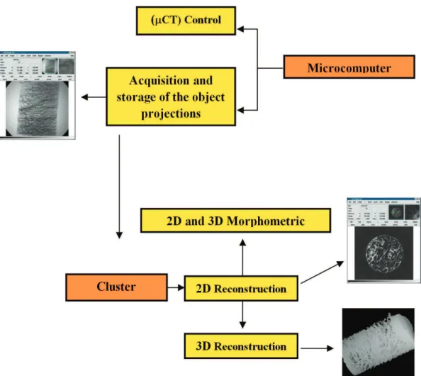
The steps for the acquisition of cross-sections and morphometric analysis by µCT of a trabecular bone sample are shown in Figure 2, in summary, include the following steps:

The Morphometric Analysis by μCT is performed

using the reconstruction of the 2D cross-sections of the sample (2D analysis) or 3D volume reconstruction of the sample (3D analysis), as described by Hildebrand et al. (1999). The parameters are calculated using stereological techniques and assuming that bone sample has a microstructure composed of plates or

rods (Feldkamp et al. 1989). The formulations of equations were originally developed for conventional histomorphometry and continue to be used in 2D

µCT analysis. The algorithm calculates the input parameters for the equations (bone surface area - BS, bone volume – BV, tissue sample volume - TV “bone volume plus the pore volume”) counting the number

of pixels across the histogram (levels of gray scale in the image) which can be seen in white is characterized like bone and black as pores.

Thus, are determined the following parameters:

Trabecular Thickness (Tb.Th):It is the average

thickness of the trabeculae. The measurement unit is mm. Equations 3 and 4 are used considering the plate or rod model, respectively, to represent the trabeculae (CT-Analyser, 2008; Silva et al., 2011):

2 .

( / )

Tb Th

BS BV

= (plate model) (3)

4 .

( / )

Tb Dm

BS BV

= (rod model) (4)

where BS / BV is the ratio of bone surface and bone volume.

Trabecular Number (Tb.N):It is the number of

trabeculae per unit of length. The unit of measurement is mm-1. Equations 5 and 6 are used for the calculation in the plate or rod model, respectively, to represent the trabeculae (CT-Analyser, 2008; Silva et al., 2011):

(

/

)

. . BV TV Tb N Tb Th

= (plate model) (5)

4 . . BV TV Tb N Tb Dm   _×        π 

= (rod model) (6)

where BV / TV is the ratio of bone volume and tissue volume.

Trabecular Separation (Tb.Sp):It is the main

diameter of the cavities containing the bone marrow. The measurement unit is mm. Equations 7 and 8 are used for the calculation in the plate and rod model, respectively, to represent the trabeculae (CT-Analyser, 2008; Silva et al., 2011):

1

. .

.

Tb Sp Tb Th

Tb N

= − (plate model) (7)

4

. . BV 1

Tb Sp Tb Dm

TV

 __{  } __ 

(3)

The 3D Morphometric Analysis is not based on a structural model of plates or rods and all the measurements of parameters, including the primaries (bone surface (BS); bone volume (BV); tissue volume (TV)) are performed directly from the volume of bone reconstructed of sample. The (BS) measurement is calculated using the method of “Marching Cubes” which is performed by placing triangles to the bone surface sample (Lorensen and Cline, 1987; Muller et al., 1994). The (BV) measurement

is calculated using tetrahedrons built in triangle’s

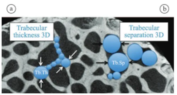
surface (Guilak, 1994). And TV is determined by a count of voxels. To compare samples with different sizes are used standardized indexes (BV/TV), (BS/ TV) and (BS/BV). The parameter (Tb.Th) is calculated using spheres in which the diameter must satisfy the structure of the trabeculae (Hildebrand et al. 1999). In the calculating of parameter (Tb.Sp) is used the same principle of determining (Tb.Th) in the voxels that contains the bone marrow (Figure 3). The parameter (Tb.N), Figure 4, is the inverse of the distance between

the main axes (center lines) of the bone trabeculae (CT-Analyser, 2008; Silva et al., 2011).

Whitehouse (1974) described the measurement of microstructural anisotropy using a counting technique of intersections, expressed by the measurement of length the main intersection (mean intercept length, MIL). The MIL principle is the counting of the intersections number between parallel lines grid and interface trabeculae/marrow on a trabecular bone

lat section. Whitehouse noted these points could be

interpolated accurately and represented by an ellipse. The generalization of the structural anisotropy creates a three-dimensional ellipsoid.

The general equation of an ellipsoid in a Cartesian Coordinate System with axes x, y and z is given by:

2 2 2

2 2 2 1

Ax +By +Cz + Dxy+ Exz+ Fyz= (9)

Let L(θ) the (MIL) calculated in θ direction in α

plane with arbitrary direction. The α plane intercepts a bone sample generating a section. Let n₁, n₂ and n₃

(4)

projections on the x, y and z coordinate system, of a

unit vector n with θ direction belonging to the α plane.

Is a vector with L(θ) magnitude in the direction of

the unit vector n of the α plane. The coordinates of

the vector with L(θ) magnitude on the x, y and z axes are given by: x = L(θ) n1, y = L(θ) n2 and z = L(θ) n3.

The Equation 9 can be rewritten as:

2 2 2

1 2 3 1 2 1 3 2 3 2

1

2 2 2

( )

An Bn Cn Dn n En n Fn n

L

+ + + + + =

θ (10) The Equation 10, in a matrix form, can be rewritten as:

[

1 2 3

]

12 2

3 1

. .

( )

A D E n

n n n D B F n

L

E F C n

     _{   =}

    _θ

       

(11)

Where M is a positive deinite second-order tensor,

expressed by 3×3 matrix of the Equation 11, and n is a

unit vector that deines the direction on which to infer the value of L(θ). The tensor M, named anisotropy

tensor, features the geometric arrangement of the porous media microstructure. The eigenvectors of M provide the main directions of the ellipsoid, which are the main orientations of trabeculae. Harrigan and Mann (1984) proposed an experimental technique for

measuring L(θ) in an arbitrary direction and MIL in

three dimensions. The technique consists in obtaining ellipses on three mutually orthogonal planes of the sample, which are the orthogonal projections of an ellipsoid about these plans.

The Degree of Anisotropy (DA) is deined by:

min 1

max

eigenvalue DA

eigenvalue

  

=_ _{− } __

   (12)

Using the minimum and maximum eigenvalues of the M matrix, the values for the degree of anisotropy can range from 0 (indicating the structure is completely isotropic) to 1 (indicating the structure is completely anisotropic). The main directions of the ellipsoid, which are the preferred orientations of the trabeculae, depend upon the number of distinct eigenvalues obtained from analysis. If all the eigenvalues of M are different, the MIL is represented by an ellipsoid with three principal axes with different sizes and the porous media has an orthotropic symmetry. If two of the three eigenvalues are equal, the MIL is represented by an ellipsoid with two main equal sizes axes and features transversely isotropic symmetry of porous media. If all M eigenvalues are equal, the MIL is represented by a sphere and the porous media has an isotropic symmetry (Cowin, 1985; Cowin and Mehrabadi, 1989).

Methods

Three pairs of bovine femurs from the same breed, with approximate ages and weights were supplied by the company Barra Mansa Comércio de Carnes e Derivados LTDA, city of Sertãozinho, São Paulo. The femurs were kept in a freezer at –20 °C until used for extraction of trabecular bone samples.

The extraction of the eighteen bone samples with 10 mm diameter by 20 mm height was performed in the “Biomechanics Laboratory,” at Instituto de Ortopedia e Traumatologia do Hospital das Clínicas da Faculdade de Medicina da USP (IOT-HC-FMUSP) and mechanical workshop at Escola de Engenharia de Sao Carlos-USP (OME). The following procedures were used to extract samples of bovine femur:

Procedure 1: Extraction of trabecular cubic sample in 3 steps.

• Step 1: Radiography of femurs for viewing

the alignment of trabecular bone in the craniocaudal direction and alignment of the femur to the cuts of samples;

• Step 2: Marking distances of approximately

30 mm in the femoral head, to designate the cuts;

Figure 3. Schematic drawing of the principle of determination (Tb. Th) in A, and (Tb.Sp) in B, by 3D analysis.

(5)

• Step 3: Femoral head cuts in the transverse

and perpendicular directions, determination of cubic sample.

Procedure 2: Extraction in each cubic bone sample of three cylindrical samples in 4 steps. Extraction was carried out in mechanical workshop at EESC-USP. The cylinders with 10 mm diameter and 20 mm height were taken on the main direction of trabeculae.

• Step 1: Fixation of cannula trephine in a radial

drill (Silva, 2009), and pitch adjustment of drilling (0.187 mm) and rotation (60 rpm). The penetration and rotation step of the drill were chosen to minimize the temperature increase at cube sample (maximum 47 °C to avoid necrosis of bone tissue (Eriksson and Albrektsson, 1984)) and possible structure damage;

• Step 2: Cube sample attachment at bench vise

and trephine positioning;

• Step 3: Cube sample drill (keeping irrigated

with distilled water) (Alves, 1996) and monitoring of the temperature with a digital temperature sensor: power 1 mW, accuracy of ± 0.5 °C, red wavelength output 630-670 nm (MT-350 model, Minipa, Brazil);

• Step 4: Cylindrical sample withdrawal with the

trephine and storage with saline (0.9% NaCl) kept in the refrigerator until the morphometric analysis by µCT (Silva, 2009).

The 2D projections acquisition and reconstruction of trabecular cylindrical samples were performed by X-ray microtomograph (1172 model, SkyScan, Belgium) at EMBRAPA Instrumentação Agropecuária (São Carlos-SP). The 2D and 3D morphometric analyzes used the CT-Analyser software provided by manufacturer (SkyScan).

The following procedures were performed during

the microstructural quantiication:

• Procedure 1: Fixation of cylindrical sample

in a circular support with play dough;

• Procedure 2: Projections acquisition from

the central region of the cylindrical samples and reconstruction of 936 cross sections in TIF/16 bits format with 6,96 µm resolution;

• Procedure 3: The 2D and 3D morphometric

analysis of 201 cross sections of central region bone sample.

Statistical Analysis was performed with the Statistica software (version 8.0) using the Pearson correlation test and the paired t-test to compare 2D and 3D measurements of the following microstructural parameters: trabecular thickness, trabecular number, trabecular separation. The anisotropy in 3D dimension was also measured.

Results

Table 1, 2 and 3 describe the average value of the morphometric parameters from the 2D and 3D analyzes measured on each main direction, respectively. Example of 2D and 3D images from the CT-Analyser and CT-Vol softwares, respectively, are shown in Figure 5. The better correlation is between the 2D trabecular thickness (rod model) and the 3D trabecular thickness measurements.

Table 4 describes the paired t-test, with signiicance

level of 0.5% (p < 0.05) in 2D and 3D analyzes, showing the statistical similarity and difference among the measures. The test was applied to the following morphometric parameters: trabecular thickness, trabecular separation, trabecular number, and eigenvalues of the M matrix (anisotropy tensor).

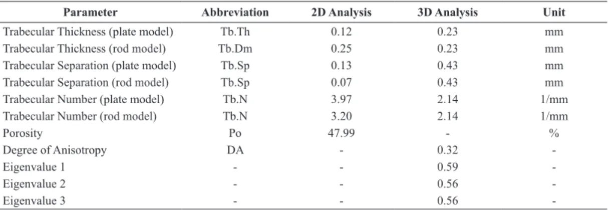
Table 1. Mean values of morphometric parameters (n = 6) from the 2D and 3D analysis (direction cranio-caudal).

Parameter Abbreviation 2D Analysis 3D Analysis Unit

Trabecular Thickness (plate model) Tb.Th 0.12 0.23 mm

Trabecular Thickness (rod model) Tb.Dm 0.25 0.23 mm

Trabecular Separation (plate model) Tb.Sp 0.13 0.43 mm

Trabecular Separation (rod model) Tb.Sp 0.07 0.43 mm

Trabecular Number (plate model) Tb.N 3.97 2.14 1/mm

Trabecular Number (rod model) Tb.N 3.20 2.14 1/mm

Porosity Po 47.99 - %

Degree of Anisotropy DA - 0.32

-Eigenvalue 1 - - 0.59

(6)

-The Statistical Analysis of parameters shows the differences between 2D and 3D Analyzes except for parameter of trabecular thickness in the rod model. And for 3D Analyze the eigenvalue

1 becomes distinct among the eigenvalues of the matrix M (tensor anisotropy) indicating a tendency to transversely isotropic symmetry overall bone structure (macroscale).

Table 2. Mean values of morphometric parameters (n = 5) from the 2D and 3D analysis (direction medial-lateral).

-Table 3. Mean values of morphometric parameters (n = 5) from the 2D and 3D analysis (direction anterior-posterior).

(7)

Discussion

The 2D (plate model) and 3D comparative analysis of the trabecular thickness parameter showed a

statistically signiicant difference (p = 0; Table 4).

However the 2D (rod model) and 3D measurement of the trabecular thickness did not show a statistically

signiicant difference (p = 0.26) meaning that the 2D

measurement (rod model) is a good approximation of the 3D measurement.

For the trabecular separation parameter, 2D and 3D, comparative analysis realized a statistically

signiicant difference (p = 0), showing that both

measurements, plate model and rod model, were not good approximations in the 3D measurement.

The trabecular number values showed a statistically

signiicant difference (p = 0) when the plate and the

rod model measurements were compared with the 3D measurements. However, there was a strong correlation between the plate and the rod model measurements.

The statistical difference observed for the eigenvalues of the M matrix (anisotropy tensor) showed that the eigenvalue 1 is distinct from eigenvalue 2 and 3 and therefore the trabecular bovine bone microstructure had a tendency to present transversely isotropic symmetry (Cowin, 1985; Cowin and Mehrabadi, 1989).

The analyzes based on 2D measurements depend on the region of interest (ROI) chosen in the images making the choice of the ROI a complex procedure. If the sample has a ROI whose microstructure is not the same throughout the sections, the results may lead to false interpretation. Otherwise the 3D measurement responds better to the morphology of the sample, performed by voxels representation of volume, providing all necessary spatial information for the morphometric parameters calculated (Lima et al., 2009). To base results upon average values may

not be the best solution, but when the format of the microstructure remains along the sections (in case of the ROI with a same circumference in the entire structure), observe that the average 2D analysis for the rod model trabecular thickness, is roughly the same of 3D analysis.

It has been observed that not only the bone mineral density (BMD) but also the morphology of the bone structure (symmetry) plays an important role in bone toughness. Luo et al (1999) showed that the BMD contributes with about 65% of the variation in bone strength, but 90% explanation of this variation can be reached if the contribution of the microarchitecture is taken into account in the analysis. In this sense a more detailed study of trabecular morphometry began to raise a great interest in the medical community for seeking more accurate measurements for the osteoporosis diagnosis and treatment (Chapard et al., 1999). The characterization of bone quality can be improved by adding microstructural and mechanical information.

It is possible to use a mechanical test module coupled to microtomograph in order to determine mechanical and microstructural correlations, which to improves the characterization of bone quality by adding a number of structural and mechanical values to BMD, obtaining a better diagnosis of entire bone structure degradation, and the consequent drop in mechanical structural toughness, thus indicating a possible incidence of metabolic bone diseases such as osteoporosis.

Acknowledgements

We wish to thank the Coordenação de Aperfeiçoamento de Pessoal de Nível Superior (Capes) for the master degree fellowship, the Fundação de Amparo a

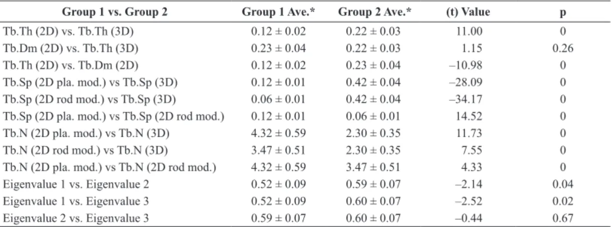
Table 4. Paired t-test (p <0.05) morphometric parameters (n = 16).

Group 1 vs. Group 2 Group 1 Ave.* Group 2 Ave.* (t) Value p

Tb.Th (2D) vs. Tb.Th (3D) 0.12 ± 0.02 0.22 ± 0.03 11.00 0

Tb.Dm (2D) vs. Tb.Th (3D) 0.23 ± 0.04 0.22 ± 0.03 1.15 0.26

Tb.Th (2D) vs. Tb.Dm (2D) 0.12 ± 0.02 0.23 ± 0.04 –10.98 0

Tb.Sp (2D pla. mod.) vs Tb.Sp (3D) 0.12 ± 0.01 0.42 ± 0.04 –28.09 0

Tb.Sp (2D rod mod.) vs Tb.Sp (3D) 0.06 ± 0.01 0.42 ± 0.04 –34.17 0

Tb.Sp (2D pla. mod.) vs Tb.Sp (2D rod mod.) 0.12 ± 0.01 0.06 ± 0.01 14.52 0

Tb.N (2D pla. mod.) vs Tb.N (3D) 4.32 ± 0.59 2.30 ± 0.35 11.73 0

Tb.N (2D rod mod.) vs Tb.N (3D) 3.47 ± 0.51 2.30 ± 0.35 7.55 0

Tb.N (2D pla. mod.) vs Tb.N (2D rod mod.) 4.32 ± 0.59 3.47 ± 0.51 4.33 0

Eigenvalue 1 vs. Eigenvalue 2 0.52 ± 0.09 0.59 ± 0.07 –2.14 0.04

(8)

Pesquisa do Estado de São Paulo (FAPESP) for the grant research # 08/56563-5, the Escola de Engenharia de São Carlos - Universidade de São Paulo, the Instituto de Ortopedia e Traumatologia, Faculdade de Medicina - Universidade de São Paulo, the EMBRAPA Instrumentação Agropecuária and the Programa de Pós-Graduação Interunidades Bioengenharia - Universidade de São Paulo for the facilities to carry out this investigation.

References

Alves JM. Caracterização do tecido ósseo por ultra-som para diagnóstico de osteoporose [thesis]. São Carlos: Instituto de Física de São Carlos; 1996.

Carter DR, Hayes WC. The compressive behavior of bone as a two-phase porous structure. Journal of Bone and Joint Surgery. 1977; 59A:954-62.

Chapard D, Legrand E, Pascaretti C, Baslé MF, Audran M. Comparison of eight histomorphometric methods for measuring trabecular bone architecture by image analysis on histological sections. Microscopy Research and Technique. 1999; 45:303-12. http://dx.doi.org/10.1002/ (SICI)1097-0029(19990515/01)45:4/5<303::AID-JEMT14>3.0.CO;2-8

Ciarelli MJ, Goldstein SA, Kuhn JL, Cody DD, Brown MB. Evaluation of orthogonal mechanical properties and density of human trabecular bone from the major methaphyseal regions with materials testing and computed tomography. Journal of Orthopaedic Research. 1991; 9:674-82. PMid:1870031. http://dx.doi.org/10.1002/jor.1100090507

Cowin SC. The relationship between the elasticity tensor and the fabric tensor. Mechanics of Materials. 1985; 4:137-47. http://dx.doi.org/10.1016/0167-6636(85)90012-2

Cowin SC, Mehrabadi MM. Identification of the elastic symmetry of bone and other materials. Journal of Biomechanics. 1989; 22(6); 503-15. http://dx.doi. org/10.1016/0021-9290(89)90001-8

CT-Analyser. Bone biology user guide. Belgium: Skyscan; 2008.

Currey JD. The mechanical consequences of variation in the mineral content of bone. Journal of Biomechanics. 1969; 2:1-11. http://dx.doi.org/10.1016/0021-9290(69)90036-0

Eriksson AR, Albrektsson T. The effect of heat on bone regeneration: an experimental study in the rabbit using the bone growth chamber. Journal of Oral and Maxillofacial Surgery. 1984; 42(11):705-11. http://dx.doi.org/10.1016/0278-2391(84)90417-8

Feldkamp LA, Godstein SA, Parfitt AM, Jesion G, Kleerekoper M. The direct examination of three-dimensional bone architecture in vitro by computed tomography. Journal of Bone and Mineral Research. 1989; 4:3-11. PMid:2718776. http://dx.doi.org/10.1002/jbmr.5650040103

Goulet RW, Goldstein SA, Ciabelli MJ, Kuhn JL, Brown MB, Feldkamp LA. The relationship between the structural and orthogonal compressive properties of trabecular bone.

Journal of Biomechanics. 1994; 27:375-89. http://dx.doi. org/10.1016/0021-9290(94)90014-0

Guilak F. Volume and surface area of viable chondrocytes in situ using geometric modeling of serial confocal sections, Journal of Microscopy. 1994; 173:245-56. PMid:8189447. http://dx.doi.org/10.1111/j.1365-2818.1994.tb03447.x

Harrigan T, Mann RW. Characterization of microstructural anisotropy in orthotropic materials using a second rank tensor. Journal of Materials Science. 1984; 19:761-7. http:// dx.doi.org/10.1007/BF00540446

Hildebrand T, Laib A, Muller R, Dequeker J, Ruegsegger P. Direct three-dimensional morphometric analysis of human cancellous bone: Microstructural data from spine, femur iliac crest and calcaneus. Journal of Bone and Mineral Research. 1999; 14(7):1167-74. PMid:10404017. http:// dx.doi.org/10.1359/jbmr.1999.14.7.1167

Kinney JH, Lane NE, Haupt DL. In-vivo, three-dimensional microscopy of trabecular bone, Journal of Bone and Mineral Research. 1995; 10(2):264-70. PMid:7754806. http://dx.doi. org/10.1002/jbmr.5650100213

Kuhn JL, Goldstein SA, Feldkamp LA, Goulet RW, Jesion G. Evaluation of a microcomputed tomography system to study trabecular bone structure. Journal of Orthopaedic Research. 1990; 8:833-42. PMid:2213340. http://dx.doi. org/10.1002/jor.1100080608

Lima I, Lopes RT, Oliveira LF, Alves JM. Análise de estrutura óssea através de microtomograia computadorizada 3D. Revista Brasileira de Física Médica. 2009; 2(1):6-10.

Lorensen WE, Cline HE. Marching cubes: A high resolution 3D surface construction algorithm. Computer Graphics. 1987; 21:163-9. http://dx.doi. org/10.1145/37402.37422

Luo G, Kinney JH, Kaufman JJ, Haupt D, Chiabrera A, Siffert RS. Relationship between plain radiographic patterns and three-dimensional trabecular architecture in the human. Osteoporosis International. 1999; 9:339-45. PMid:10550451. http://dx.doi.org/10.1007/s001980050156

Majumdar S, Bay BK. Noninvasive assessment of trabecular bone architecture and the competence of bone. Kluwer Academic, Plenum Publishers; 2001. p. 240. http://dx.doi. org/10.1007/978-1-4615-0651-5

Mccreadie B, Goldstein SA. Biomechanics of fracture: Is bone mineral density suficient to assess risk? Journal of Bone and Mineral Research. 2000; 15(12):2302-8. PMid:11127195. http://dx.doi.org/10.1359/jbmr.2000.15.12.2305

Muller R, Hildebrand T, Ruegsseger P. Non-invasive bone biopsy: a new method to analyse and display the three-dimensional structure of trabecular bone. Physics in Medicine and Biology. 1994; 29:145-64. http://dx.doi. org/10.1088/0031-9155/39/1/009

(9)

Rice JC, Cowin SC, Bowman JA. On the dependence of elasticity and strength of cancellous bone on apparent density. Journal of Biomechanics. 1988; 21:155-68. http:// dx.doi.org/10.1016/0021-9290(88)90008-5

Silva AMH, Alves JM, Da Silva OL, Ferreira NJ, Gazziro M, Pereira JC, Lasso PRO, Vaz CMP, Pereira CAM, Leiva TP, Guarniero R. Microstructural assessment of cancellous bone using 3D microtomography. Journal of Physics. Conference Series (Online). 2011; 313:1-10.

Silva AMH. Análise morfométrica 2D e 3D de amostras de osso trabecular utilizando microtomograia tridimensional por raios-X [dissertation]. São Carlos: Escola de Engenharia de São Carlos, 2009.

Roque WL, Souza ACA, Barbieri DX, Rodrigue FC. Um sistema computacional baseado no brocessamento de imagens

tomográicas para estudo da estrutura trabecular. In: VI Simpósio Brasileiro de Qualidade de Software; VII Workshop de Informática Médica: Anais do Simpósio Brasileiro de Qualidade de Software e Workshop de Informática Médica; 2007; Porto de Galinhas. Porto de Galinhas; 2007. p. 156-65. Relatório Final.

Rüegsegger P, Koller B, Müller R. A microtomographic system for the nondestructive evaluation of bone architecture. Calciied Tissue International. 1996; 58:24-29. PMid:8825235. http://dx.doi.org/10.1007/BF02509542

Whitehouse WJ. The quantitative morphology of anisotropic trabecular bone. Journal of Microscopy. 1974; 101:153-68. PMid:4610138. http://dx.doi.org/10.1111/j.1365-2818.1974. tb03878.x

Authors

Alessandro Márcio Hakme da Silva, Orivaldo Lopes da Silva, Nelson Ferreira da Silva Junior, José Marcos Alves PPGIBiongenharia, Escola de Engenharia de São Carlos, Faculdade de Medicina de Ribeirão Preto, Instituto de Química de São Carlos, Universidade de São Paulo - EESC/FMRP/IQSC - USP, Av. Trabalhador Saocarlense, 400, Centro, 13566-590, São Carlos, São Paulo, Brasil

José Marcos Alves