Abstract
The current study presents an enhanced biogeography-based opti-mization (EBBO) algorithm for size and shape optiopti-mization of truss structures with natural frequency constraints. The BBO algorithm is one of the recently developed meta-heuristic algorithms inspired by the mathematical models in biogeography science and is based on the migration behavior of species among the habitats in the na-ture. In this study, the overall performance of the standard BBO algorithm is enhanced by new migration and mutation operators. The efficiency of the proposed algorithm is demonstrated by utiliz-ing four benchmark truss design examples with frequency con-straints. Numerical results show that the proposed EBBO algorithm not only significantly improves the performance of the standard BBO algorithm, but also finds competitive results compared with recently developed optimization methods.
Keywords
Biogeography-based optimization, meta-heuristic, truss structures, dynamic constraints, size and shape optimization.
Enhanced Biogeography-based Optimization: A New
Method for Size and Shape Optimization of Truss
Structures with Natural Frequency Constraints
1 INTRODUCTION
The ability to control and modify the values of free vibrational frequencies and corresponding mode shapes in structures is a significant issue to keep their vibrational performance desirable. In most of the low frequency vibration problems, the response of the structure to dynamic excitation is primarily a function of its fundamental frequency and mode shapes (Grandhi, 1993). Particularly, this is an important issue when a certain excitation frequency can cause resonance phenomena in the structure. Therefore, structural optimization with natural frequency constraints has important applications in manipulating the dynamic performance of the structures.
Seyed Heja Seyed Taheri a Shahin Jalili b
a Islamic Azad University, Urmia, Iran.
b Young Researchers and Elite Club,
mia Branch, Islamic Azad University, Ur-mia, Iran. [email protected]
http://dx.doi.org/10.1590/1679-78252208
From optimization point-of-view, size optimization of truss structures with frequency constraints is described as highly non-linear and non-convex optimization problem with several local optimums in its search space. On the other hand, if the shape variables, beside the size variables, are considered to resolve this problem, the optimization problem will become more complex, and the associative performance will degrade seriously. The main reason for this complexity is related to the different physical representation of these variables, and sometimes their changes are of widely different orders of magnitude (Wang et al., 2004). Therefore, the size and shape optimization of truss structures with frequency constraints is one of the active areas in the research of structural optimization at present.
Generally, two main approaches are available in the literature to address the structural optimi-zation problem with frequency constraints. These approaches are the conventional optimioptimi-zation tech-niques based on the use of classical gradient-based optimization techtech-niques, and the meta-heuristic search methods based on the use of nature-inspired stochastic optimization algorithms. Nevertheless, the conventional methods such as the optimality criteria (OC) and mathematical programming (MP), need complex and time-consuming dynamic sensitivity analysis and are easily trapped into local op-timum (Lingyun et al., 2005). On the other hand, the meta-heuristic search methods such as the genetic algorithms (GAs) (Goldberg, 1989), particle swarm optimization (PSO) (Eberhart and Ken-nedy, 1995), big bang-big crunch (BB-BC) algorithm (Erol and Eksin, 2006), gravitational search algorithm (GSA) (Rashedi et al., 2009), biogeography-based optimization (BBO) (Simon, 2008; Jalili et al., 2015), Cultural Algorithm (CA) (Reynolds, 1999; Jalili and Hosseinzadeh, 2015), and charged system search (CSS) algorithm (Kaveh and Talatahari, 2010) require less computational effort and can also find near-optimum solutions in a relatively reasonable time. Therefore, meta-heuristic opti-mization techniques are usually preferred to conventional approaches, and in most cases, show much better performances. However, it is widely believed that the overall performance of heuristic search methods mainly depends on the type of the optimization problem and the features of its search space. Hence, extensive studies have been carried out to develop efficient heuristic optimization methods for size and shape optimization of truss structures with natural frequency constraints, ranging from hy-brid techniques to enhanced versions of standard algorithms. The Democratic PSO (DPSO) algorithm (Kaveh and Zolghadr, 2014a), hybrid CSS-BBBC algorithm (Kaveh and Zolghadr, 2012), enhanced CSS algorithm (Kaveh and Zolghadr, 2011), niche hybrid genetic algorithm (NHGA) (Lingyun et al., 2005), and orthogonal multi-gravitational search algorithm (OMGSA) (Khatibinia and Naseralavi, 2014) are some instances of these methods.
migration operator. In addition, the simple and purely random mutation operator of the BBO may lead to revisiting non-productive regions of the search space. In this study, in order to enhance the performance of standard BBO algorithm, new migration and mutation operators are proposed. These new migration and mutation operators improve the convergence properties of the BBO algorithm and enhance the algorithm’s ability to further escape stagnation and premature convergence. To evaluate the efficiency of the proposed algorithm, four benchmark truss design examples with frequency con-straints are investigated and the results generated by the EBBO algorithm are compared with the results of several other state-of-the-art methods. Numerical results show that the proposed EBBO algorithm not only significantly improves the standard BBO algorithm, but also finds competitive results compared with recently developed optimization methods for truss optimum design problem with frequency constraints.
The remaining sections complete the presentation of this paper as followings. Section 2 formulates the optimum design problem of truss structures with frequency constraints. In Section 3, the BBO algorithm is first reviewed and then, the proposed EBBO algorithm is explained in detail. Four benchmark truss design examples are optimized by utilizing the proposed algorithm in Section 4. Finally, the concluding remarks are presented in Section 5.
2 TRUSS OPTIMUM DESIGN PROBLEM
The main purpose of this optimum design problem is to minimize the weight of the structure under some frequency constraints. In the layout and size optimization of truss structures, the cross sectional areas and the coordinates of nodes are considered as design variables. Thus, the optimal design of a truss structure with frequency constraints can be formulated as:
Find:
, , … ,To minimize:
Cost .Subjected to:
(1)max , max , (2)
where α is a constant value and nc and is the number of frequency constraints. The parameter α has a major effect on the algorithm’s performance. At the initial stages of the optimization process, the value of this parameter should be small enough to explore the whole search space (exploration), while whatever the optimization process closes to the final stages, it should be large enough to provide more focus on the feasible solutions (exploitation). In this study, the value of α in Eq. (2) starts from 2 and linearly increases to 7 by lapse of the iteration (Kaveh and Zolghadr, 2014b) as follows:
=2+ (3)
where It and Itmaxare the current iteration number and maximum considered iterations, respectively.
3 OPTIMIZATION METHOD
3.1 Biogeography-Based Optimization
The Biogeography-based optimization (BBO) method inspired by biogeography science is a recently developed meta-heuristic algorithm which has been introduced by Simon (2008).The biogeography sci-ence describes the geographical distribution of biological organisms in nature. The overall framework of this algorithm is developed based on the probabilistic mathematical models of biogeography science. These mathematical models were developed by MacArthur and Wilson (1967) and explain how species migrate between the habitats. In the BBO algorithm, each habitat (Hi) is a solution candidate for the
optimization problem and the position of each habitat (Hi) in an n-dimensional search space represented
by Suitability Index Variables (SIVs), which is an n-dimensional vector. The quality of each habitat is measured by the Habitat Suitability Index (HSI), which is directly proportional to the fitness function value. Thus, the habitats with high HSI values are better solutions than the ones with low HSI values. The BBO algorithm consists of two main operators: migration and mutation.
This algorithm utilizes migration operator as a powerful tool to share information between habi-tats in the solution space. So, it can be considered as an exploitation mechanism during the optimi-zation process. The migration operator shares information between habitats based on immigration
and emigration rates, probabilistically. Each habitat has its own immigrationǺi and
emigra-tion ǻi rates which are the functions of species in the habitat. For a given habitat, the immigration Ǻi
rate is inversely proportional to the HSI (fitness) value, while the emigration ǻi rate is directly
pro-portional to HSI value. The habitats with high immigration rates (poor solutions) are more likely to accept information from the other habitats with high HSI values, while the habitats with low immi-gration rates (good solutions) share their information with other poor habitats with a high probability. The immigration and emigration rates are calculated for each habitat as follows (Simon, 2008):
(4)
(5)
where I is the maximum possible immigration rate; E is the maximum possible emigration rate; K is the number of species in the ith habitat; and Smax is the maximum number of species. These
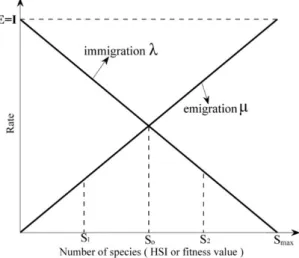
imgration and emiimgration rates are calculated based on the miimgration models. There are different mi-gration models that can be utilized to calculate the immimi-gration and emimi-gration rates. Figure 1 shows the simple linear migration model for the case E=I. According to Figure 1, the habitats with a high HSI value tend to have a large number of species, while those with a low HSI have a small number of species (Simon, 2008). From Figure 1, it can be concluded that the habitat with few species (poor solution, low HSI) like S1, has a low emigration rate and a high immigration rate. This means that,
the habitat with low HSI tends to take information about the good habitats with the high probability, while the probability of sharing its information for other habitats is relatively low. On the other hand, the habitat which has more species (good solution, high HSI) like S2, has a low immigration rate and
a high emigration rate. Such habitats with high HSI values share their information with the other habitats with a high probability. By utilizing this mechanism, the migration operator of the BBO algorithm can achieve adequate exploitation ability between the habitats in the search space. For each variable of a given solution (Hi), the immigration Ǻi rate decides whether or not to immigrate.
If the immigration condition is satisfied, the migration procedure occurs between the immigrating and emigrating habitats as follows:
⟵ (6)
Eq. (6) explains that one of the variables of ith habitat is replaced by a variable of jth habitat. Here, and are the immigrating and emigrating habitats, respectively. It is worth mentioning that the emigrating habitat ( ) is selected based on the emigration rates . The probability of selecting jth habitat as emigrating habitat is calculated as follow:
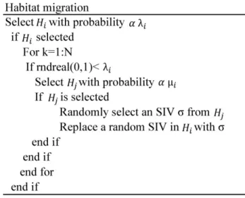
where NP is the population size. Figure 2 demonstrates the details of the migration procedure in the
BBO algorithm. Here, the roulette wheel selection technique is used to select emigrating habitat.
Figure 2: The migration procedure of the BBO algorithm.
In most cases, it is possible that a meta-heuristic algorithm is trapped to the local optimum by lapse of the iteration. In order to escape from the local traps in the search space, the BBO algorithm utilizes a mutation operator. Mutation operator is a probabilistic operator that modifies a habitat’s SIV randomly based on mutation rate ( ), which is related to the habitat’s probability. The mutation rate for each habitat is calculated as follows:
(8)
where is a user-defined parameter and = max . More details about the calculation of and probabilities can be found in (Simon, 2008). Based on Eq. (8), a variable of each habitat mutates randomly in search space with a given probability. For a better explanation, the mutation operator of the BBO algorithm can be described as in Figure 3. In this study, for simplicity, the probability of performing mutation operator for the all habitats is set to 0.1 . .
Another feature of the BBO algorithm is that the elite habitats with high HSI values are selected to keep and transfer from previous generation to the current one. Therefore, the Keeprate parameter is defined for this purpose. In this study, 20% (Keeprate=0.2) of habitats with high HSI values are selected to keep in each generation. It means that the 20% of elite habitats from the previous popu-lation are transferred to the current generation and combined with new habitats. Finally, the habitats with high HSI values are selected from the combined population of habitats to form a new population.
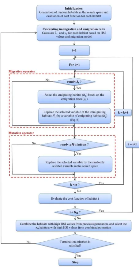
For a better explanation, Figure 4 shows the flowchart of the standard BBO algorithm.
3.2 Enhanced Biogeography-Based Optimization
As mentioned before, the standard BBO algorithm may not be successful in finding better solutions for some non-linear complicated optimization problems. The main reason for this issue is that the basic BBO algorithm employs simple migration and mutation operators during the optimization pro-cess. Such simple operators may lead to some disadvantages such as a low exploration ability and premature convergence. In a migration operator, the immigrating habitat is updated by simply re-placing one of the SIV of emigrating habitat randomly, which often implies a rapid loss of diversity in the population. With the aim of achieving a better exploitation capability and providing efficient information sharing between the habitats, the new migration operator is proposed as follows:
⟵ Φ Φ (9)
where and are the immigrating and emigrating habitats, respectively, Φ is a random number uniformly generated between the 0 and 1, and denotes the best position experi-enced by the emigrating habitat. As it can be seen from Eq. (9), the new migration operator changes a variable of ith habitat by considering both current and best positions of the emigrating habitat. The proposed migration scheme has an important role in achieving an efficient exploitation ability.
On the other hand, the purely random mutation operator of the standard BBO algorithm may lead to revisiting non-productive regions of the search space, which leads to weak exploration ability, excessive computational efforts, and long computing time. Therefore, in order to enhance the explo-ration ability and eliminate the effect of the purely random mutation, following mutation operator is proposed:
⟵ ,
, I
t=1,2,3, … ,
(10)In order to better explain, the main steps of the proposed EBBO algorithm can be listed as below: Step 1: Initialization
In the first step, the random habitats are generated in the search space as follows:
Φ (11)
where Φ is the random number uniformly distributed between 0 and 1. Then, the value of HSI or cost function value is calculated for each habitat.
Step 2: Calculating immigration and emigration rates
In this step, the immigration and emigration rates are calculated for each habitat based on the migration model (Figure 1) and HSI values.
Step 3: Migration procedure
In the third step, the migration procedure is performed based on the immigration and emigra-tion rates for each habitat by utilizing Eq. (9).
Step 4: Mutation procedure
After migration procedure, the variables of each habitat mutate with constant probability ( pMu-tation) by Eq. (10).
Step 5: Evaluation of HSI values
In this step, the HSI values of the new generated habitats are computed. Step 6: Formation of new population of habitats
A specific number of elite habitats from the previous population (KeepRate×NP) are transferred
to the current generation and combined with the new habitats. Finally, the habitats with high HSI values are selected from the combined population of habitats to form a new population.
Step 7: Finish or redoing
Repeat from Steps 2–6 until the stopping criteria is met and output the best solution.
4 NUMERICAL EXAMPLES
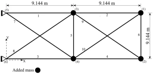
Figure 5:Schematic of 10-bar planar truss structure.
4.1 A 10-Bar Planar Truss Structure
The 10-bar planar truss structure with fixed configuration shown in Figure 5 is the first example. Young’s modulus is 6.89×10¹⁰ N/m2 and material density of truss members is2770.0 kg/m3. As seen in Figure 5, a non-structural mass of 454.0 kg is attached to all free nodes of the structure. The lower and upper bounds for the cross-sectional areas are specified as 0.645 cm2 and 50 cm2, respectively. The three natural frequency constraints are considered as: Hz, Hz, Hz. It is worth mentioning that, in some of the previous researches, the Young’s modulus of the truss members is given as 6.98× N/m . So, for a fair comparison, we considered two cases as follows: E= 6.89×10¹⁰ N/m2 (Case 1) and E= 6.98×10¹⁰ N/m2 (Case 2).
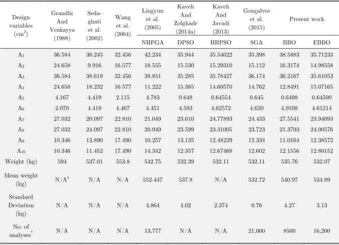
For Case 1, the optimum designs obtained through various methods are tabulated in Table 1, wherein the best design is ensured by the EBBO algorithm. From Table 1, it can be seen that the EBBO algorithm not only yields a better design than the SGA method, but it also requires signifi-cantly less structural analyses. However, the values of standard deviation and average weight are larger compared to the SGA method. In addition, Table 2 presents the frequencies of the structure obtained by various methods at the optimum designs. According to Table 2, it can be concluded that the designs reported by Sedaghati et al. (2002) and HRPSO violate the design constraints.
Design variables
(cm2)
Grandhi And Venkayya (1988) Seda-ghati et al. (2002) Wang et al. (2004) Lingyun et al. (2005) Kaveh And Zolghadr (2014a) Kaveh And Javadi (2013) Gonçalves et al. (2015) Present work
NHPGA DPSO HRPSO SGA BBO EBBO
A1 36.584 38.245 32.456 42.234 35.944 35.54022 35.398 38.5883 35.71233
A2 24.658 9.916 16.577 18.555 15.530 15.29310 15.112 16.3174 14.98558
A3 36.584 38.619 32.456 38.851 35.285 35.78427 36.174 36.2167 35.61053
A4 24.658 18.232 16.577 11.222 15.385 14.60570 14.762 12.8491 15.07165
A5 4.167 4.419 2.115 4.783 0.648 0.64554 0.645 0.6498 0.64500
A6 2.070 4.419 4.467 4.451 4.583 4.62572 4.620 4.9108 4.61214
A7 27.032 20.097 22.810 21.049 23.610 24.77893 24.433 27.5541 23.94093
A8 27.032 24.097 22.810 20.949 23.599 23.31005 23.723 21.3793 24.00576
A9 10.346 13.890 17.490 10.257 13.135 12.48229 12.334 11.0164 12.38572
A10 10.346 11.452 17.490 14.342 12.357 12.67468 12.602 12.1556 12.80152
Weight (kg) 594 537.01 553.8 542.75 532.39 532.11 532.11 535.76 532.07
Mean weight
(kg) N/A
a N/A N/A 552.447 537.8 N/A 532.72 540.97 534.89
Standard Deviation (kg)
N/A N/A N/A 4.864 4.02 2.374 0.76 4.27 3.13
No. of
analyses* N/A N/A N/A 13,777 N/A N/A 21,000 8500 16,200
* Number of analyses corresponding to the best result during 100 independent runs.
Table 1:Comparison of the optimal designs obtained by different methods for the 10-bar planar truss structure (Case 1).
Frequency No. Grandhi and Venkayya (1988) Seda-ghati et al. (2002) Wang et al. (2004) Lingyun et al. (2005) Kaveh and Zolghadr (2014a) Kaveh and Javadi (2013) Gonçalves et al. (2015) Present work
NHPGA DPSO HRPSO SGA BBO EBBO
1 7.059 6.992 7.011 7.008 7.000 6.9999 7.0001 7.0456 7.0000 2 15.895 17.599 17.302 18.148 16.187 16.1752 16.1912 16.3072 16.1812
3 20.425 19.973 20.001 20.000 20.000 19.9999 20.0000 20.1299 20.0001 4 20.425 19.977 20.100 20.508 20.021 20.0060 20.0048 20.4485 20.0014 5 20.425 28. 173 30.869 27.797 28.470 28.5156 28.4758 27.7338 28.5019
6 30.189 31.029 32.666 31.281 29.243 28.9837 28.8965 29.0805 29.0158 7 54.286 47.628 48.282 48.304 48.769 48.5734 48.6102 48.9125 48.6089 8 56.546 52.292 52.306 53.306 51.389 51.0823 51.0822 51.8780 51.1237
Design variables (cm2)
Gomes
(2011) Kaveh and Zolghadr (2012)
Kaveh And Javadi (2013) Gonçalves et al. (2015) Present work
PSO CSS E-CSSa
CSS-BBBC HRPSO SGA BBO EBBO
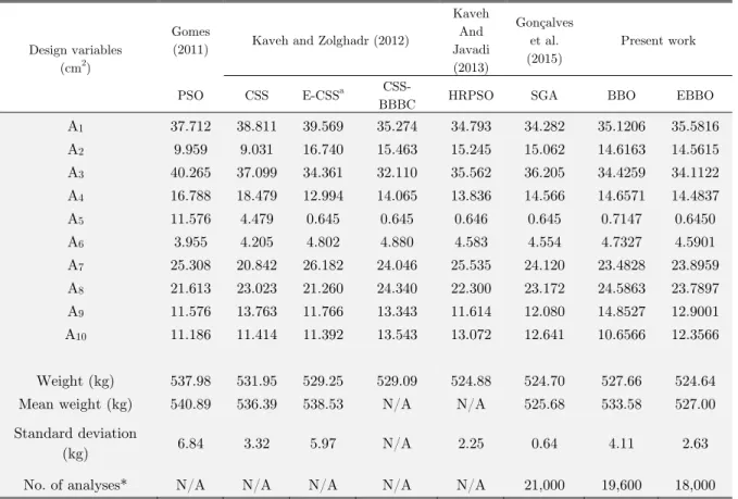
A1 37.712 38.811 39.569 35.274 34.793 34.282 35.1206 35.5816
A2 9.959 9.031 16.740 15.463 15.245 15.062 14.6163 14.5615
A3 40.265 37.099 34.361 32.110 35.562 36.205 34.4259 34.1122
A4 16.788 18.479 12.994 14.065 13.836 14.566 14.6571 14.4837
A5 11.576 4.479 0.645 0.645 0.646 0.645 0.7147 0.6450
A6 3.955 4.205 4.802 4.880 4.583 4.554 4.7327 4.5901
A7 25.308 20.842 26.182 24.046 25.535 24.120 23.4828 23.8959
A8 21.613 23.023 21.260 24.340 22.300 23.172 24.5863 23.7897
A9 11.576 13.763 11.766 13.343 11.614 12.080 14.8527 12.9001
A10 11.186 11.414 11.392 13.543 13.072 12.641 10.6566 12.3566
Weight (kg) 537.98 531.95 529.25 529.09 524.88 524.70 527.66 524.64
Mean weight (kg) 540.89 536.39 538.53 N/A N/A 525.68 533.58 527.00
Standard deviation
(kg) 6.84 3.32 5.97 N/A 2.25 0.64 4.11 2.63
No. of analyses* N/A N/A N/A N/A N/A 21,000 19,600 18,000
a Enhanced CSS; * Number of analyses corresponding to the best result during 100 independent runs.
Table 3: Comparison of the optimal designs obtained by different methods for the 10-bar planar truss structure (Case 2).
Frequency No.
Gomes
(2011) Kaveh and Zolghadr (2012)
Kaveh and Javadi (2013)
Gonçalves
et al.(2015) Present work
PSO CSS E-CSS
CSS-BBBC HRPSO SGA BBO EBBO
1 7.000 7.000 7.000 7.000 7.0000 7.0003 7.0006 7.0000
2 17.786 17.442 16.238 16.119 16.1686 16.2033 16.2650 16.1575
3 20.000 20.031 20.000 20.075 20.0015 20.0002 20.0472 20.0000
4 20.063 20.208 20.361 20.457 20.0050 20.0121 20.2079 20.0038
5 27.776 28.261 28.121 29.149 28.1466 28.4621 27.7244 28.6433
6 30.939 31.139 28.610 29.761 29.2724 28.9983 30.2389 29.1169
7 47.297 47.704 48.390 47.950 48.5235 48.6445 48.4195 48.3767
8 52.286 52.420 52.291 51.215 50.9950 51.1643 51.0860 50.9613
Finally, the convergence characteristic of the BBO and EBBO algorithms for two cases are dis-played in Figures 6 and 7. As it can be seen, the proposed algorithm reaches the near-optimum solution after 4000 analyses evaluated in 100 independent runs, while this value for standard BBO algorithm is about over 8000 analyses.
Figure 6: The Convergence diagrams of the EBBO and standard BBO algorithms for the 10-bar planar truss structure (Case 1).
4.2 A Simply Supported 37-Bar Planar Truss Structure
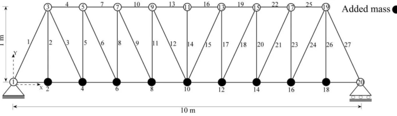
The second design example is the size and shape optimization of a simply supported 37-bar planar truss structure shown in Fig. 8. Young’s modulus and material density of truss members are2.1×1011 N/m and 7800 kg/m3, respectively. A non-structural mass of 10 kg is attached to free nodes at the lower chord of the structure. The constant rectangular cross-sectional areas of 4×10⁻³ m2 are specified for all members of the lower chord and the cross-sectional areas of other members are considered as design variables. By considering geometrical symmetry, the y-coordinates of upper nodes are taken as layout variables and their vertical position can vary between ±1.5 m. Moreover, this structure is subject to the first three frequency constraints as follows: ω Hz, ω Hz, ω Hz.
Figure 8: Schematic of the simply supported 37-bar planar truss structure.
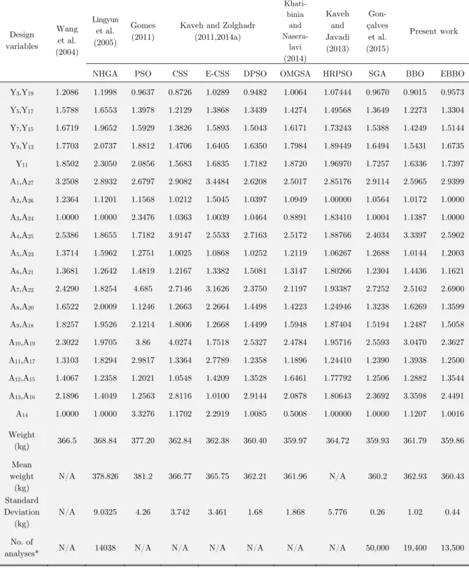
Design variables Wang et al. (2004) Lingyun et al. (2005) Gomes (2011)
Kaveh and Zolghadr (2011,2014a) Khati-binia and Nasera-lavi (2014) Kaveh and Javadi (2013) Gon-çalves et al. (2015) Present work
NHGA PSO CSS E-CSS DPSO OMGSA HRPSO SGA BBO EBBO
Y3,Y19 1.2086 1.1998 0.9637 0.8726 1.0289 0.9482 1.0064 1.07444 0.9670 0.9015 0.9573
Y5,Y17 1.5788 1.6553 1.3978 1.2129 1.3868 1.3439 1.4274 1.49568 1.3649 1.2273 1.3304
Y7,Y15 1.6719 1.9652 1.5929 1.3826 1.5893 1.5043 1.6171 1.73243 1.5388 1.4249 1.5144
Y9,Y13 1.7703 2.0737 1.8812 1.4706 1.6405 1.6350 1.7984 1.89449 1.6494 1.5431 1.6735
Y11 1.8502 2.3050 2.0856 1.5683 1.6835 1.7182 1.8720 1.96970 1.7257 1.6336 1.7397
A1,A27 3.2508 2.8932 2.6797 2.9082 3.4484 2.6208 2.5017 2.85176 2.9114 2.5965 2.9399
A2,A26 1.2364 1.1201 1.1568 1.0212 1.5045 1.0397 1.0949 1.00000 1.0564 1.0172 1.0000
A3,A24 1.0000 1.0000 2.3476 1.0363 1.0039 1.0464 0.8891 1.83410 1.0004 1.1387 1.0000
A4,A25 2.5386 1.8655 1.7182 3.9147 2.5533 2.7163 2.5172 1.88766 2.4034 3.3397 2.5902
A5,A23 1.3714 1.5962 1.2751 1.0025 1.0868 1.0252 1.2119 1.06267 1.2688 1.0144 1.2003
A6,A21 1.3681 1.2642 1.4819 1.2167 1.3382 1.5081 1.3147 1.80266 1.2304 1.4436 1.1621
A7,A22 2.4290 1.8254 4.685 2.7146 3.1626 2.3750 2.1197 1.93387 2.7252 2.5162 2.6900
A8,A20 1.6522 2.0009 1.1246 1.2663 2.2664 1.4498 1.4223 1.24946 1.3238 1.6269 1.3599
A9,A18 1.8257 1.9526 2.1214 1.8006 1.2668 1.4499 1.5948 1.87404 1.5194 1.2487 1.5058
A10,A19 2.3022 1.9705 3.86 4.0274 1.7518 2.5327 2.4784 1.95716 2.5593 3.0470 2.3627
A11,A17 1.3103 1.8294 2.9817 1.3364 2.7789 1.2358 1.1896 1.24410 1.2390 1.3938 1.2500
A12,A15 1.4067 1.2358 1.2021 1.0548 1.4209 1.3528 1.6461 1.77792 1.2506 1.2882 1.3544
A13,A16 2.1896 1.4049 1.2563 2.8116 1.0100 2.9144 2.0878 1.80643 2.3692 3.3598 2.4491
A14 1.0000 1.0000 3.3276 1.1702 2.2919 1.0085 0.5008 1.00000 1.0000 1.1207 1.0016
Weight
(kg) 366.5 368.84 377.20 362.84 362.38 360.40 359.97 364.72 359.93 361.79 359.86
Mean weight
(kg)
N/A 378.826 381.2 366.77 365.75 362.21 361.96 N/A 360.2 362.93 360.43
Standard Deviation
(kg)
N/A 9.0325 4.26 3.742 3.461 1.68 1.868 5.776 0.26 1.02 0.44
No. of
analyses* N/A 14038 N/A N/A N/A N/A N/A N/A 50,000 19,400 13,500
* Number of analyses corresponding to the best result during 100 independent runs.
Frequency No.
Wang et al. (2004)
Lingyun et al. (2005)
Gomes
(2011) Kaveh and Zolghadr (2011,2014a)
Khatibinia and Naseralavi
(2014)
Present work
NHGA PSO CSS E-CSS DPSO OMGSA BBO EBBO
1 20.0850 20.0013 20.0001 20.0000 20.0028 20.0194 20.0220 20.04197 20.0005
2 42.0743 40.0305 40.0003 40.0693 40.0155 40.0113 40.0100 40.05697 40.0008 3 62.9383 60.0000 60.0001 60.6982 61.2798 60.0082 60.0490 60.07207 60.0039 4 74.4539 73.0444 73.0440 75.7339 78.1100 76.9896 76.4510 78.40251 76.3152 5 90.0576 89.8244 89.8240 97.6137 98.4100 97.2222 96.2970 97.99689 96.3553
Table 6:Comparison of the frequencies (Hz) obtained by different methods for the simply supported 37-bar planar truss structure.
Figure 9: The Convergence diagrams of the EBBO and standard BBO algorithms for the simply supported 37-bar truss structure.
Figure 9 demonstrates convergence diagrams of the standard BBO and EBBO algorithms for the simply supported 37-bar planar truss structures. With regard to Figure 9, it is clear that the conver-gence speed of the EBBO algorithm is faster than that of the standard BBO algorithm. The EBBO algorithm reaches to the vicinity of final optimum solution after about 6000 analyses, while this value for the standard BBO algorithm is about 14,000 analyses. In addition, Figure 10 indicates the com-parison of the initial and optimized shapes at the best design for this design example.
Element group
Kaveh and Zolghadr (2014a,2012)
Khatibinia and Naseralavi
(2014)
Present work
CSS
CSS-BBBC PSO DPSO OMGSA BBO EBBO
1 21.710 17.478 23.494 19.6070 20.2630 18.2999 19.8878
2 40.862 49.076 32.976 41.2900 39.2940 44.4985 39.8248
3 9.048 12.365 11.492 11.1360 9.9890 9.8161 10.5496
4 19.673 21.979 24.839 21.0250 20.5630 20.4079 21.0929
5 8.336 11.190 9.964 10.0600 9.6030 10.9003 9.4245
6 16.120 12.590 12.039 12.7580 11.7380 13.4254 11.6648
7 18.976 13.585 14.249 15.4140 15.8770 14.8123 15.1282
Weight (kg) 9204.51 9046.34 9171.93 8890.48 8724.97 8776.3 8711.95
Mean weight (kg) N/A N/A 9251.84 8895.99 8745.58 8916.9 8718.5
Standard deviation
(kg) N/A N/A 89.38 4.26 1.18 128.63 7.15
No. of analyses* N/A N/A N/A N/A N/A 29,850 6500
Table 7:Comparison of the optimal designs obtained by different methods for the 120-bar dome truss structure.
Frequency No.
Kaveh and Zolghadr (2014a,2012) Khatibinia and
Naseralavi (2014) Present work
CSS
CSS-BBBC PSO DPSO OMGSA BBO EBBO
1 9.002 9.000 9.0000 9.0001 9.002 9.0001 9.0000
2 11.002 11.007 11.0000 11.0007 11.003 11.0007 11.0000
3 11.006 11.018 11.0052 11.0053 11.003 11.0007 11.0002
4 11.015 11.026 11.0134 11.0129 11.007 11.0015 11.0002
5 11.045 11.048 11.0428 11.0471 11.076 11.0735 11.0657
*Number of analyses corresponding to the best result during 100 independent runs
4.3 A 120-Bar Dome Truss Structure
The third example is a 120-bar dome truss structure shown in Figure 11. The members of this struc-ture are divided into 7 groups based on symmetry. The minimum and maximum cross-sectional areas for each group of members are 1 cm2 and 129.3 cm2, respectively. Young’s modulus and material density of truss members are2.1×1011 N/m2and 7971.810 kg/m3, respectively. Non-structural masses are attached to all free nodes as follows: 3000 kg at node one, 500 kg at nodes 2 through 13 kg and 100 kg at the rest of the nodes. In addition, the structure is subject to frequency constraints as:
9 H , Hz.
Figure 12: The Convergence diagrams of the EBBO and standard BBO algorithms for the 120-bar dome truss structure.
Group number Members Group number Members
1 1, 2, 3, 4 15 102, 105, 108, 111, 114
2 5, 8, 11, 14, 17 16 82, 83, 85, 86, 88, 89, 91, 92, 103,
104, 106, 107, 109, 110, 112, 113
3 19, 20, 21, 22, 23, 24 17 115, 116, 117, 118
4 18, 25, 56, 63, 94, 101, 132, 139,
170, 177 18 119, 122, 125, 128, 131
5 26, 29, 32, 35, 38 19 133, 134, 135, 136, 137, 138
6 6, 7, 9, 10, 12, 13, 15, 16, 27, 28,
30, 31, 33, 34, 36, 37 20 140, 143, 146, 149, 152
7 39, 40, 41, 42 21
120, 121, 123, 124, 126, 127, 129, 130, 141, 142, 144, 145, 147, 148,
150, 151
8 43, 46, 49, 52, 55 22 153, 154, 155, 156
9 57, 58, 59, 60, 61, 62 23 157, 160, 163, 166, 169
10 64, 67, 70, 73, 76 24 171, 172, 173, 174, 175, 176
11 44, 45, 47, 48, 50, 51, 53, 54, 65,
66, 68, 69, 71, 72, 74, 75 25 178, 181, 184, 187, 190
12 77, 78, 79, 80 26
158, 159, 161, 162, 164, 165, 167, 168, 179, 180, 182, 183, 185, 186,
188, 189
13 81, 84, 87, 90, 93 27 191, 192, 193, 194
14 95, 96, 97, 98, 99, 100 28 195, 197, 198, 200
29 196, 199
The obtained results through different optimization methods for this structure are summarized in Table 7. According to this table, one can observe that the design obtained by the EBBO algorithm is better than all the other methods. Although the value of standard deviation of the EBBO algorithm is larger than the values obtained by the OMGSA and DPSO methods, but the EBBO algorithm is more efficient than these methods in the term of the average of the results. In addition, it is important to note that the standard BBO algorithm obtained better results than the CSS, CSS-BBBC, PSO, and DPSO methods. However, it requires significantly more structural analyses than the EBBO al-gorithm. Moreover, the frequencies evaluated by different methods for the dome truss structure are listed in Table 8. As it can be seen, the values of the first two frequencies are very close to the allowable values.
Figure 12 illustrates the convergence diagrams of the standard BBO and EBBO algorithms for the 120-bar dome truss structure. As it can be observed, the convergence rate of the EBBO algorithm is considerably faster than the standard BBO algorithm. The proposed algorithm reaches to the vicinity of the final solution after about 5000 analyses evaluated in 100 independent runs without any abruption.
Element group Kaveh and Zolghadr (2012)
Khatibinia and Naseralavi
(2014)
Present work
CSS CSS-BBBC OMGSA BBO EBBO
1 1.2439 0.2934 0.2890 0.1980 0.3059
2 1.1438 0.5561 0.4860 0.5928 0.4539
3 0.3769 0.2952 0.1000 1.6883 0.1000
4 0.1494 0.1970 0.1000 0.9960 0.1000
5 0.4835 0.8340 0.4990 1.4562 0.5210
6 0.8103 0.6455 0.8040 0.9733 0.8260
7 0.4364 0.1770 0.1030 0.7371 0.1000
8 1.4554 1.4796 1.3770 1.5266 1.4619
9 1.0103 0.4497 0.1000 0.1751 0.1001
10 2.1382 1.4556 1.5540 1.1536 1.5839
11 0.8583 1.2238 1.1510 1.2562 1.1426
12 1.2718 0.2739 0.1310 0.9819 0.1028
13 3.0807 1.9174 3.0280 3.0189 2.9913
14 0.2677 0.1170 0.1010 0.2562 0.1000
15 4.2403 3.5535 3.2610 1.8976 3.3607
16 2.0098 1.3360 1.6120 2.4537 1.5674
17 1.5956 0.6289 0.2090 1.1546 0.2825
18 6.2338 4.8335 5.0200 4.4126 5.1062
19 2.5793 0.6062 0.1330 0.5324 0.1000
20 3.0520 5.4393 5.4530 5.4785 5.4145
21 1.8121 1.8435 2.1130 4.0169 2.1388
22 1.2986 1.8435 0.7230 1.3088 0.7121
23 5.8810 8.1759 7.7240 6.1357 7.6374
24 0.2324 0.3209 0.1820 1.8785 0.1151
25 7.7536 10.9800 7.9710 8.1935 7.9160
26 2.6871 2.9489 2.9960 4.3817 2.8073
27 12.5094 10.5243 10.2060 11.5248 10.2844
28 29.5704 20.4271 20.6990 20.3022 21.2686
29 8.2910 19.0983 11.5550 12.1376 10.7450
Weight (kg) 2559.86 2298.61 2158.64 2539.85 2156.81
Mean weight (kg) N/A N/A 2167.53 2727.10 2157.80
Standard deviation (kg) N/A N/A 1.5860 85.18 1.25
No.of required analyses N/A N/A N/A 29,100 16,500
4.4 A 200-Bar Planar Truss Structure
The last design example is a 200-bar planar truss structure shown in Figure 13. The Young’s modulus is 2.1×10¹¹ N/m2 and the material density of truss members is 7860 kg/m3. The minimum permitted cross-sectional area for the truss members is considered as 0.1cm2. A non-structural mass of 100 kg is attached to the nodes at the top of the structure. In addition, the structure is subject to the first three frequency constraints as: ω Hz, ω Hz, ω Hz. The members of the structure are divided into 29 groups as shown in Table 9. This example has 29 design variables and it is considered a high dimensional optimization problem.
Table 10 compares the designs founded by the standard BBO and EBBO algorithms with other methods in the literature. With regard to the results given in Table 10, it is clear that the proposed EBBO algorithm obtained the lowest structural weight tan the CSS, CSS-BBBC, and OMGSA meth-ods. In addition, the EBBO algorithm is more efficient than the OMGSA method in terms of average and standard deviation. Moreover, it can be seen from Table 10 that the standard BBO algorithm obtained better design than the CSS algorithm. Furthermore, the frequencies of the structure evalu-ated at the optimum designs are given in Table 11. Also, the design obtained by the EBBO algorithm is feasible, i.e., the constraints are not violated.
Frequency No. Kaveh and Zolghadr (2012)
Khatibinia and Naseralavi
(2014)
Present work
CSS CSS-BBBC OMGSA BBO EBBO
1 5.000 5.010 5.000 5.0067 5.0000
2 15.961 12.911 12.118 13.8669 12.2666
3 16.407 15.416 15.029 15.0755 15.0766
4 20.748 17.033 16.639 17.0058 16.7338
5 21.903 21.426 21.218 20.5140 21.4288
6 26.995 21.613 21.420 23.6846 21.5080
Table 11:Comparison of the frequencies (Hz) obtained by different methods for the 200-bar planar truss structure.
Figure 14: The Convergence diagrams of the EBBO and standard BBO algorithms for the 200-bar planar truss structure.
5 CONCLUSIONS
The Biogeography-Based Optimization (BBO) is a simple and recently introduced meta-heuristic optimization algorithm. The basic concepts and ideas of the method are inspired by the mathematical models in biogeography science and are based on migration behavior of species among habitats in the nature. The algorithm consists of two main operators: migration and mutation. In most cases, the standard BBO algorithm may fail to find the best solution. The main reason for this issue is that the basic BBO algorithm employs simple migration and mutation operators during the optimization pro-cess. Herein, an effective algorithm, called the Enhanced BBO (EBBO), has been developed to miti-gate premature convergence problem of the standard BBO algorithm. In the proposed algorithm, to enhance the overall performance of the standard BBO algorithm, the new migration and mutation operators are proposed. The new migration and mutation operators improve the convergence proper-ties of the BBO algorithm and enhance the algorithm’s ability to further escape stagnation and premature convergence. To evaluate the performance of the proposed algorithm, four benchmark truss design examples with frequency constraints are investigated and the results are compared with those of the standard BBO algorithm and other methods in literature. The computational experiments show that the presented EBBO algorithm can get better solutions, and it is more efficient than the standard BBO algorithm on the size and shape optimization of truss structures problems with frequency con-straints. Moreover, it can be stated that the proposed algorithm is straightforward and free of com-putational complexity.
References
Boussaid, I., Chatterjee, A., Siarry, P., Ahmed-Nacer, M., 2012. Biogeography-based optimization for constrained optimization problems. Computers & Operations Research 39(12):3293–3304.
Eberhart, R.C., Kennedy, J., 1995. A new optimizer using particle swarm theory. Proceedings of the Sixth International Symposium on Micro Machine and Human Science, Nagoya, Japan.
Erol, O.K., Eksin, I., 2006. New optimization method: big bang-big crunch. Advances in Engineering Software 37:106– 111.
Goldberg, D.E. 1989. Genetic Algorithms in Search Optimization and Machine Learning, Addison-Wesley, Boston. Gomes, M.H., 2011. Truss optimization with dynamic constraints using a particle swarm algorithm, Expert Systems with Applications 38:957–968.
Goncalves, MS., Lopez, RH., Miguel, LFF., 2015. Search group algorithm: a new meta-heuristic method for the opti-mization of truss structures. Computers & Structures 153:165–184.
Grandhi, R.V. 1993. Structural optimization with frequency constraints—a review. AIAA Journal 31:2296–2303. Jalili, S., Hosseinzadeh, Y., 2015. A cultural algorithm for optimal design of truss structures. Latin American Journal of Solids and Structures. 12:1721-1747.
Jalili, S., Hosseinzadeh, Y., Taghizadieh, N., 2015. A biogeography-based optimization for optimum discrete design of skeletal structures. Engineerng Optimization. DOI: 10.1080/0305215X.2015.1115028.
Kaveh A, Javadi, SM., 2013. Shape and sizing optimization of trusses with multiple frequency constraints using har-mony search and ray optimizer for enhancing the particle swarm optimization algorithm. Acta Mechanica 225: 1595-1605.
Kaveh, A., Zolghadr, A., 2011. Shape and size optimization of truss structures with frequency constraints using en-hanced charged system search algorithm. Asian Journal of Civil Engineering 12:487–509.
Kaveh, A., Zolghadr, A., 2012. Truss optimization with natural frequency constraints using a hybridized CSS–BBBC algorithm with trap recognition capability, Computers and Structures 102-103:14-27.
Kaveh, A., Zolghadr, A., 2014a. Democratic PSO for truss layout and size optimization with frequency constraints. Computers & Structures 130:102–103.
Kaveh, A., Zolghadr, A., 2014b. Comparison of nine meta-heuristic algorithms for optimal design of truss structures with frequency constraints. Advances in Engineering Software 76:9-30.
Kaveh, A.,Talatahari, S., 2010. A novel heuristic optimization method: charged system search. Acta Mechanica 213:267–286.
Khatibinia, M., Sadegh Naseralavi, S., 2014. Truss optimization on shape and sizing with frequency constraints based on orthogonal multi-gravitational search algorithm. Journal of Sound and Vibration. 333:6349–6369.
Lingyun, W., Mei, Z., Guangming, W., Guang, M., 2005. Truss optimization on shape and sizing with frequency constraints based on genetic algorithm. Computational Mechanics 25:361–368.
MacArthur, R., Wilson, E., 1967. The Theory of Biogeography, Princeton University Press; USA.
Miguel, LFF. 2013. Shape and size optimization of truss structures considering dynamic constraints through modern metaheuristic algorithms. Expert Systems with Applications 39:9458–9467.
Rashedi, E., Nezamabadi-pour, H., Saryazdi, S., 2009. GSA: a gravitational search algorithm. Information Science 179: 2232–2248.
Reynolds, R.G., 1999. Cultural Algorithms: Theory and Application. In D. Corne, M. Dorigo, and F. Glover, edi-tors, New Ideas in Optimization, pages 367–378. McGraw-Hill.
Sedaghati, R., Suleman, A., Tabarrok, B., 2002. Structural optimization with frequency constraints using finite element force method. AIAA Journal 40:382–388.
Simon, D., Rarick, R., Ergezer, M., Du, D. 2011. Analytical and numerical comparisons of biogeography-based opti-mization and genetic algorithms. Information Sciences 181(7):1224–1248.
Singh, U., Kumar, H., Kamal, T., 2010. Design of Yagi-Uda Antenna Using Biogeography Based Optimization. IEEE Transactions on Antennas and Propagation. 58(10):3375–3379.