Lat. Am. j. solids struct. vol.11 número7

(1)

Abstract

This study presents an alternative Finite Element formulation

based on positions to model plane frames considering geometrical

non_-_{linear and elastoplastic behavior for members and semi}_-_rigid

connections. The formulation includes shear effects and allows the

consideration of important mechanical behavior of structures in

design decisions and verifications. The principle of stationary

energy is used to find the equilibrium equations. A multi-linear

elastoplastic constitutive law is developed for both continuum

members and semi_-_{rigid connections in order to comprise any}

proposed stress-strain diagram. Large rotations and displacements

are considered for both semi_-_{rigid connections and structure. The}

most important steps used to derive the formulation are described along the paper and various examples are used to validate and show the possibilities of the proposed technique.

Key words

Frames, Physical and geometrical non-linear analysis, Positional

FEM, Elastoplastic connections, Laminate cross sections.

Physical and geometrical non-linear analysis of plane

frames considering elastoplastic semi-rigid connections

by the positional FEM

1 INTRODUCTION

Computational technology improvements provide a continuous advance in structural analysis, resulting in designs of lighter and slender structures. In this sense, the geometrical and physical non-linear analysis of structures, including any kind of flexible connection, acquire special im-portance in engineering analysis. From this reasoning it is necessary to develop a well-posed non linear formulation allowing the accurate evaluation of displacements and efforts of conventional and unconventional structures.

Various researches related to geometrical non linear analysis of two and three-dimensional frames that consider plasticity can be cited. Some pioneering authors as Shi and Atluri (1988) and Argyris et al (1982) applied co-rotational techniques to analyze three-dimensional frames developing plasticity. In these works elastoplasticity were treated in a discrete way (plastic

hing-Ma rce lo Ca mp os J un qu e ira Re isa H um berto Breves C od aa , *

a

Structural Engineering Department, Escola de Engenharia de São Carlos, Universidade de São Paulo

*

(2)

Latin American Journal of Solids and Structures 11 (2014) 1163-1189

es), in which a moment-curvature relation is assumed for continuous members cross sections. One can cite some recent works that follows the same localized plastic hinge strategy to model the behavior of frame elements, are they: Zhou and Chan (2004), Ren et al (1999), Armero and Ehr-lich (2006), EhrEhr-lich and Armero (2005), White (1993), Chen et al (1996), Landesmann and Batis-ta (2005), Chan and Zhou (2004) and Ngo-Huu et al (2007).

Some authors as Alvarenga and Silveira (2009), Avery and Mahendran (2000) and Gruttmann et al (2000) use distributed plasticity to model two and three dimensional frames. One advantage of distributed plasticity, when compared to plastic hinges, is the better representation of the plas-tic evolution over cross sections, without the necessity of a previous knowledge of moment-curvature curves. However, both plastic hinges and the existent distributed plasticity frame mod-els do not consider the shear stress influence as the finite element proposed in this work.

Concerning problems in which semi-rigid connections are present one can cite the works of Lui and Chen (1988), King (1994), Simões (1996), Chui and Chan (1997), Xu (2001), Sekulovic and Salatic (2001), Pinheiro (2003), Kruger et al. (1995) and Chan and Chui (2000). All these works use second order geometrical description, which limits the range of applications, i.e., displace-ments and rotations should not be large.

In order to implement semi-rigid connections in any computational code it is necessary to use results from works that study the experimental behavior of these connection, as, for example, Chen and Kishi (1989) and Abdalla and Chen (1995). Some works that, using experimental re-sults, try to establish empirical mathematical models for connections behavior are also present in literature see, for example, the works of Richard and Abbott (1975), Frye and Morris (1975), Ang and Morris (1984), Lui and Chen (1986), Lui and Chen (1988), Kishi and Chen (1986a), Kishi and Chen (1986b) and Zhu et al. (1995). In our work, as an alternative to these empirical formu-las, we propose a multi-linear elastoplastic diagram that allows to follow the experimental results for semi-rigid connections. Moreover the elastoplastic behavior ensures realistic results for cycling loads that are not provided by the non-linear elastic empirical formulas proposed by the previous-ly mentioned works.

In the present work an alternative position based Finite Element (FE) formulation (Bonet et al., 2000 and Coda and Greco, 2004) is developed to comprise geometrical and physical non-linearity of both frame members and connections. The formulation, originally developed and pre-sented in this work, is geometrically exact and, considering the Reissner kinematic hypothesis, includes shear stress contribution in both displacement and failure criterion. Based on Botta et al. (2008), the developed elastoplastic algorithm is multi-linear with an alternative flow direction rule, which allow the reproduction of any stress-strain curve and the determination of closed solu-tion for the plastic multiplier. Moreover, semi-rigid elastoplastic connecsolu-tions develop large rota-tions allowing realistic analysis of unload situarota-tions for which connecrota-tions and/or frame elements suffers plastic deformations.

(3)

equations and examples are presented to validate the proposed formulation and to show its possi-bilities.

2 FRAM E ELEM ENT REISSNER KINEM ATICS

The FE formulation presented here is called positional as it is based on positions, not displace-ments (Bone et al., 2000 and Coda and Greco, 2004). The main advantage of this total lagrangian strategy is the establishment of the gradient deformation without the explicit use of the chain rule (Coda and Paccola, 2008, Coda, 2009 and Coda and Paccola, 2010). The chain rule operation appears as a simple numerical matrix inversion, which allows the generalization of this procedure for any class of non-linear mechanical problem (Coda and Paccola, 2010, Coda and Paccola, 2011, Nogueira et. al., 2012, Silva and Coda, 2013 and Pascon and Coda, 2013).

In this section we present the complete development of the alternative 2D positional Reissner kinematics to be used in the proposed finite element formulation.

2.1 Initial configuration

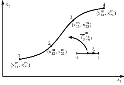
The positional formulation is based on two mappings, one related to the initial configuration and another related to the current configuration. To describe the initial configuration mapping one starts with the reference line approximation, see Figure 1, by the following expression:

f

_oim

(ξ)

=

x

_im

(ξ)

=

φ

ℓ

X

iℓ

m

(1)

in which

i

is the coordinate direction (1 or 2),

m

represents the reference line and

ℓ

the element

node (or shape function). In expression (1) the repetition of index

ℓ

_{indicates summation (Einstein} notation). Figure 1 shows 4 nodes (cubic approximation), however any quantity of nodes or approx-imation order may be chosen.

Figure 1 Reference line parameterization for initial configuration (cubic approximation)

In Figure 1

f

₀m

(

ξ

)

is the mapping from the non-dimensional variable

ξ

to the reference line. A similar mapping from the non-dimensional variable to the current reference line will be given in the next item.

2

x

x 1

1

2 3

4

11

(x , x ) 21 m m

m 12

m 22

(x , x )

m 23 m 13

(x , x )

(x , x ) 14m m 24

1 -1

ξ

(4)

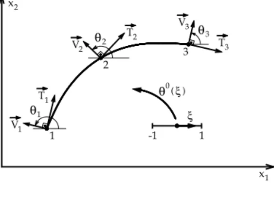
We start to build the initial configuration of the frame element writing an approximation for the normal vector, Figure 2, using the known initial reference line mapping, as follows:

Figure 2 Nodal normal vectors

The tangent vector at any point of the reference line can be written, particularly at nodes, by:

T

ik

=

d

_φ

ℓ

(

ξ

)

d

_ξ

ξk

X

iℓ m

(2)

in which

ξ

k is non-dimensional coordinate of node k and

T

ik is the

i

th component of the tangent vector at node

k

.

As a consequence, if the coordinates of reference line nodes are known, the tangent vectors at nodes are also known and the normal vectors can by calculated as:

V

1k

=

−

T

₂k

/

T

i₍k₎

T

i₍k₎ (3)

V

2k

=

T

₁k

/

T

i₍k₎

T

i₍k₎ (4)

in which index inside brackets does not mean summation, that is:

T

i(k)

T

i(k)

=

(

T

1(k)

)

2

+

(

T

2(k)

)

2

(5)

For the present positional formulation it is important to write the nodal angle

θ

k that the

normal vector

V

ik makes with the horizontal direction (

x

₁ axis), see Figure 2, as:

θ

k

0

=

arctg(V

₂₍_k₎

/

V

₁₍_k₎

)

(6)

2

x

x 1

1

3 2

2

T

2

V

V ₃

3

T

1

T

V 1

ξ ( )

0

ξ -1 1

θ θ

2 3

θ

(5)

Knowing the nodal angles we use the same shape functions to approximate

θ

0

(

ξ

)

along the initial configuration:

θ

0

(

ξ

)

₌

φ

ℓ

(

ξ

)

θ

ℓ 0

(7)

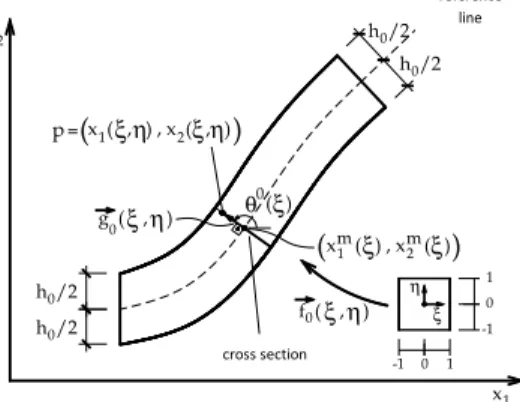
Observing Figure 3 one can find any point inside the continuum (frame) adding the normal vector

g

_i0

(

ξ

,

η

)

to a point of the reference line, as:

x

_i

(

ξ

,

η

)

=

x

_im

(

ξ

)

+

g

_i0

(

ξ

,

η

)

(8)

in which η is the second non-dimensional variable used to build the 2D frame element.

Figure 3 Point

_P

at a general cross section of the initial element configuration

Moreover, vector

g

_i0

(

ξ

,

η

)

generates cross sections with (in this paper) constant height

h

0. The width is also considered constant (

b

0) along the bar length, however it can vary along trans-verse direction to compose general cross sections. This transtrans-verse variation is opportunely intro-duced.

From Figure 3 it is established that the initial cross section is orthogonal to the reference line, so vector

g

_i0

(

ξ

,

η

)

can be written as a function of

θ

0

(ξ)

, as follows:

g

₁0

(

ξ

,

η

)

=

h

0

2 η

cos(

φ

ℓ

(

ξ

)

θ

ℓ 0

)

(9)

0 0 0

1

( , )

(

( )

)

2 h

g

ξ η

=

η

sen

φ ξ θ

_l _l (10)

in which

η

varies from

−

1

to

+

1

.

1 x x2

0 h /2 h /20

h /2 h /20 0

linh a méd

ia

seção transversal 0

g ( , )ξ η θ

0 ( )ξ

x ( ) , x ( )₁mξ 2mξ 2ξη

ξη

1

x ( , ) , x ( , )

p=( )

ξ

η 1

0 -1 0 1 -1

ξ

f ( , )0 η ) (

reference line

(6)

Substituting equations (9), (10) and (1) into (8) results the complete mapping from

₍

ξ

,

η

)

to the initial configuration of a frame element, as:

f

₀₁

(

ξ

,

η

)

₌

x

₁

(

ξ

,

η

)

₌

φ

ℓ

X

1ℓ m

+

h

0

2 η

cos(

φ

ℓ

(

ξ

)

θ

ℓ 0

)

(11)

f

₀₂

(

ξ

,

η

)

==

x

₂

(

ξ

,

η

)

=

φ

ℓ

X

2ℓ m

+

h

0

2 η

sen

(

φ

ℓ

(

ξ

)

θ

ℓ 0

)

(12)

2.2 Current configuration:

The necessary information to build the initial configuration comprises the reference line nodal coor-dinates, the height and the width of the cross section. The current configuration is achieved by a non-linear process that uses a trial position to start the solution procedure. So, we do not worry at this moment about the solution process and writes the current configuration similarly to the initial one, that is:

f

₁₁

(ξ,

η)

₌

y

₁

(ξ,

η)

₌

φ

ℓ

Y

1ℓ m

+

h

0

2 ηcos(φ

ℓ

(ξ)θ

ℓ

)

(13)

f

₁₂

(ξ,η)

₌

y

₂

(ξ,η)

₌

φ

ℓ

Y

2ℓ

m

+

h

0

2 ηsen(φ

ℓ

(ξ)θ

ℓ

)

(14)

For which

y

_i are the current coordinates of a general point inside the frame element,

Y

iℓ

m are current nodal coordinates and

θ

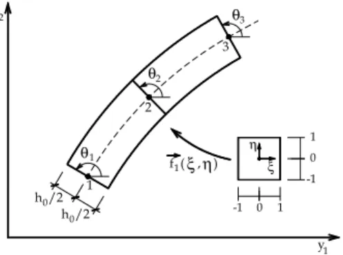
ℓ are the current angles of cross sections, see Figure 4.

Figure 4 Current configuration mapping – detaching angles

One can see from Figure 4 and from equations (13) and (14) that cross sections remain straight, but no more orthogonal to the reference line. This is the general Reissner kinematics. Moreover we kept

h

0 and

b

0 unchanged limiting our constitutive relation to accept any shear elastic modulus, but null Poisson ratio.

1

0 0 h /2 h /2

0 -1

η ξ ξ

1 f ( , )η

1

y₁ 0 -1 linha

média y₂

1

θ

1 2

θ

2

θ

3 3

(7)

2.3 Change of configuration function (deformation) and its gradient:

Being defined mappings to initial and current configurations, we start the description of the change of configuration of the analyzed body (frame). This is done by joining the two mappings of Figures 3 and 4 in a single representation, see Figure 5, for which the function

!

f

describes the change of configuration from initial configuration (

B

0) to the current one (

B

). From basic knowledge of

calculus

!

f

is written as a composition of mappings

!

f

0 and

!

f

₁ as:

!

f

₌

!

f

₁

"

(

!

f

₀

)

−1 (15)

and the gradient of

!

f

, called here

_A

(a 2x2 tensor) is written from the gradient of

!

f

0 and

!

f

₁ as:

A

=

A

1

⋅

(

A

0

)

−1 (16)

Figure 5 – Change of configuration – Positional mapping

In index notation one writes

A

_ij

=

A

_ik

D

_jk ₍₁₇₎

in which

D

_kj is the inverse of

A

kj

0

.

These gradients are written in an open form as:

A

_ij0

=

∂

f

1 0

∂ξ

∂

f

1

0

∂η

∂

f

2

0

∂ξ

∂

f

2

0

∂η

⎡

⎣

⎢

⎤

⎦

⎥

=

∂x

1

∂ξ

∂x

1

∂η

∂x

2

∂ξ

∂x

2

∂η

⎡

⎣

⎢

⎤

⎦

⎥

(18)

B

1 2

x ,x y ,y₁ ₂

f

0

B

0

f ( , )ξ η

η

f ( , )1 ξ

f ₀

( )-1

(8)

A

_ij1

=

∂

f

₁1

∂ξ

∂

f

₁1

∂η

∂

f

₂1

∂ξ

∂

f

₂1

∂η

⎡

⎣

⎢

⎤

⎦

⎥

=

∂

y

₁

∂ξ

∂

y

₁

∂η

∂

y

₂

∂ξ

∂

y

₂

∂η

⎡

⎣

⎢

⎤

⎦

⎥

(19)

Elements of

A

_ij0 and

A

_ij1 are calculated directly from expressions (11), (12), (13) and (14) for known values (integration points) of

ξ

and

η

, as:

A

11

0

=

∂

x

1

∂ξ

=

φ

ℓ,ξ

(

ξ

)

X

1ℓ m

−

h

0

2 η

sen

₍

_φ

ℓ

(

ξ

)

θ

ℓ

0

)

φ

k,ξ

(

ξ

)

θ

k 0

(20)

A

12 0

=

∂

x

1

∂η

=

h

0

2 cos(

φ

ℓ

(

ξ

)

θ

ℓ

0

)

(21)

A

21 0

=

∂

x

2

∂ξ

=

φ

ℓ,ξ

(

ξ

)

X

2ℓ m

+

h

0

2 η

cos(

φ

ℓ

(

ξ

)

θ

ℓ 0

)

φk

_,_ξ

(

ξ

)

θk

0

(22)

A

22 0

=

∂

x

2

∂η

=

h

0

2 sen

₍

_φ

ℓ

(

ξ

)

θ

ℓ 0

)

(23)

A

₁₁1

=

∂

y

1

∂ξ

=

φ

ℓ,ξ

(ξ)Y

1ℓ

m

−

h

0

2 ηsen(φ

ℓ

(ξ)θ

ℓ

)φ

k,ξ

(ξ)θ

k (24)

A

₁₂1

=

∂

y

1

∂η

=

h

₀

2 cos(φ

ℓ

(ξ)θ

ℓ

)

(25)

A

₂₁1

=

∂

y

2

∂ξ

=

φ

ℓ,ξ

(ξ)

Y

2ℓ m

+

h

0

2 ηcos(φ

ℓ

(ξ)θ

ℓ

)φ

k,ξ

(ξ)θ

k (26)

A

₂₂1

=

∂

y

2

∂η

=

h

₀

(9)

The objective Green-Lagrange strain measure

_E

is chosen to develop the geometrically exact FEM, that is:

E

₌

1

2 (

C

₋

I

₎

₌

1

2 (

A

t

A

₋

I

₎

_or

_E

ij

=

1

2 ( A

ki

A

kj

−

δ

ij

)

(28)

where

_I

is the second order identity tensor and

C

is the right Cauchy stretch.

In order to introduce lamina with different widths and material properties, one should simply change expressions (11), (12), (13) and (14) by:

x

1

(

ξ

,

η

)

=

φ

ℓ

X

₁ℓ

m

+

d

lam

+

h

0

lam

2 η

⎛

⎝⎜

⎞

⎠⎟

cos(

φ

ℓ

(

ξ

)

θ

ℓ 0

)

(29)

x

2

(

ξ

,

η

)

=

φℓ

X

2ℓ m

+

d

lam

+

h

0 lam

2 η

⎛

⎝⎜

⎞

⎠⎟

sen

(

φℓ

(

ξ

)

θℓ

0

)

(30)

y

₁

(

ξ

,

η

)

=

φ

ℓ

Y

₁ℓ

m

+

d

_lam

+

h

0 lam

2 η

⎛

⎝⎜

⎞

⎠⎟

cos(

φ

ℓ

(

ξ

)

θ

ℓ

)

(31)

y

₂

(

ξ

,

η

)

₌

φ

ℓ

Y

₂ℓ m

+

d

_lam

₊

h

0

lam

2 η

⎛

⎝⎜

⎞

⎠⎟

sen

(

φ

ℓ

(

ξ

)

θ

ℓ

)

(32)

in which

d

lam is the distance between the reference line and the concerned lamina following the positive sense of the vector defined by

θ

_{, see Figure 3. It is worth noting that}

h

0

lam

is the height of each lamina. Moreover, it is necessary to indicate the width

b

lam and the physical properties of each lamina at an integration point for which the constitutive model and the deformation gradient are required.

It is important to stress that distortion effects are naturally considered resulting in a general Reissner-Mindlin kinematics.

3 ELASTIC PROCEDURE

(10)

3.1 Elastic connections:

In order to unify the notation, the degree of freedom

θ

ℓ will be called

Y

3ℓ. Each element node has three degrees of freedom, but when connecting elements by means of semi-rigid connections (global numbering) an extremity node may have more than three degrees of freedom, as the rotations of the connected elements are not the same. Figure 6 shows three cases to illustrate the linking by means of free connections (joints).

Figure 6 Some free connections and degrees of freedom numbering.

Following Figure 6 one observes that the master element defines the first rotation degree of free-dom (the third of the node) and each slave element introduces an extra degree of freefree-dom for the connection node. Figure 7 shows the introduction of elastic connections in the structures of Figure 6.

Figure 7 Some semi-rigid connections

In general, the strain energy stored in a semi-rigid connection with stiffness modulus

k

(ηαβ) at a global node

η

- that is the initial (or final) node of a frame element

α

_{and the final (or initial)} node of a frame element

β

- is given by:

U

_ηSR

=

k

(ηαβ)

2 θ

α η

_−θ

β η

(

)

2

=

k

(ηαβ)

2 Y

3α η

₋

Y

3β

η

(

)

2

(33)

No summation implied.

kA2 3

1

θ

1

θ

2

θ

A 2

1

2

1

θ

1

3

2 B θ2

1

θ

C

1

2 k1 2 3

A 2

1

kA1 2 1 kB1 3

3

2 B

C 1

2 k1 2 3

kC2 3

12

A

k

12

B

k

12

C

k

13

B

k

23

(11)

3.2 Frame element strain energy:

As mentioned before the specific strain energy to be adopted here is the Saint-Venant-Kirchhoff one, that relates the Green strain (

_E

) and the second Piola-Kirchhoff stress (

S

) in a linear way as:

u

e

=

E

2 E

11 2

₊

_E

22 2

(

)

+

G E

12 2

₊

_E

21 2

(

)

or

u

e

=

1

2 E :

C

: E

₍₃₄₎

in which

G

=

E /

⎡⎣

₂

(

₁

+

ν

)

⎤⎦

is the shear elastic modulus,

ν

_{is the Poisson ration and}

_E

ij is the

Green strain tensor. Alternatively, in dyadic notation,

_E

is the Green strain tensor and

C

is the elastic constitutive tensor. As the Green strain has been written as a function of nodal positions, see equations (16) through (28), the strain energy stored in the bar elements is written as:

U

_e

(

!

Y )

₌

u

_e

dV

0 V0

∫

(35)

in which

V

0 is the initial volume of the analyzed structural bar elements (Coda and Greco, 2004 and Coda, 2009).

3.3 Total potential energy:

In order to write the total potential energy of the mechanical system

_Π

(

!

Y )

(conservative and isothermal) one sums the strain energy of frame elements, the strain energy of semi-rigid connec-tions, the potential energy of external loads (and moments) and the potential energy of external distributed forces, resulting:

Π

(

!

Y )

₌

u

_e

(

!

Y )dV

0

V0

∫

+

U

_eSR

₋

!

F

⋅

!

Y

−

q

!

⋅

!

y

m

(

!

Y )

S0

∫

dS

0 (36)

in which

!

F

is the external nodal force vector (including moments) and

q

!

is the general distributed force vector written as function of nodal values, by:

q

_i

=

φ

ℓ

(

ξ

)Q

ℓ_i (37)

In equation (36),

y

!

m

(

!

Y )

is the current position at the reference line of frame elements, written as function of nodal positions

Y

!

(see equations (13) and (14)) and

dS

0 is the infinitesimal length of the curved frame element.

(12)

δΠ

₌

∂

u

e

∂

_E

:

∂

_E

∂

Y

!

dV

0

⋅

δ

!

Y

V0

∫

+

∂

U

e

SR

∂

Y

!

⋅

δ

!

Y

−

!

F

⋅δ

!

Y

−

q

!

⋅

∂

!

y

m

∂

Y

!

S0

∫

dS

0

⋅δ

!

Y

=

!

0

₍₃₈₎

By the energy conjugate principle (Ogden, 1984), the first term of the first integral of equation (38) is the second Piola-Kirchhoff stress. Using the same principle, the derivative of the strain ener-gy stored in elastic connections is the internal moment

M

!

int_{. Therefore, in order to simplify the} understanding of the physical non-linear procedure, shown in next section, one rewrites equation (38) as:

δΠ

₌

S

_:

∂

E

∂

Y

!

dV

0

⋅δ

!

Y

+

V0

∫

M

!

int

⋅δ

!

Y

−

!

F

⋅δ

!

Y

−

q

!

⋅

∂

!

y

m

∂

Y

!

S0

∫

dS

0

⋅δ

!

Y

=

!

0

₍₃₉₎

The understanding of equation (39) can be further improved defining the first integral as the in-ternal nodal force and the last integral as the equivalent nodal force of applied distributed forces (Coda, 2009b), resulting:

δΠ

₌

_F

!

int

_⋅δ

!

Y

₊

!

M

int

_⋅δ

!

Y

−

_F

!

⋅δ

_Y

!

−

_L

⋅

!

Q

⋅δ

_Y

!

₌

!

0

₍₄₀₎

in which

_L

is the matrix that transforms the distributed forces into nodal equivalent ones. Due to the arbitrariness of

δ

_Y

!

_{equation (40) results into the geometrical non-linear equilibrium equation,} as:

!

F

int

+

!

M

int

−

!

F

−

L

⋅

!

Q

=

!

0

₍₄₁₎

The Newton-Raphson procedure is used to solve the non-linear equilibrium. This procedure is described in the next section, including the physical non-linear behavior of materials. To close this item we show the pair of internal moments, for an elastic semi-rigid connection, associated to a global node

η

related to the initial (or final) point of a frame element

α

_{and to the final (or} ini-tial) point of a frame element

β

, that is:

M

₃η_α

=

k

(ηαβ)

(

Y

₃η_α

−

Y

₃η_β

)

and

M

₃η_β

=

−

k

(ηαβ)

(

Y

₃η_α

−

Y

₃η_β

)

(42)

4 INELASTIC PROCEDURE

4.1 Equilibrium equation

(13)

Following this reasoning the total potential energy for isothermal problems is written as:

Π

(

!

Y )

=

Ψ

( E ,

α

)dV

0 V0

∫

+

Θ

SR

Y

3α

η

₋

Y

3β η

(

)

,

α

(

)

−

F

!

⋅

!

Y

−

q

!

⋅

y

!

m

(

!

Y )

S0

∫

dS

0 (43)

where

Ψ

and

Θ

SR_{are, respectively, the free energy potentials of the continuous (frame elements)}

and connection. These potentials are written as function of the Green strain tensor, the relative angle positions at connections and the thermodynamic parameters

α

_and

α

_.

The variation of the total potential energy is null at the equilibrium position, i.e.:

δΠ

₌

∂

Ψ

∂

_E

:

∂

_E

∂

Y

!

dV

0

⋅δ

!

Y

V0

∫

+

∂Θ

molas

∂

Y

!

⋅

δ

!

Y

−

!

F

⋅

δ

!

Y

−

q

!

⋅

∂

!

y

m

∂

Y

!

S0

∫

dS

0

⋅

δ

!

Y

=

0

₍₄₄₎

in which parameters

α

_and

α

_{are not present due to their intrinsic relation with}

_E

_and

_S

_{to be} shown in item 4.2.

Even for inelastic problems, the derivative of the free energy potential regarding Green strain is the second Piola-Kirchhoff stress tensor. For the same reason, the energy conjugate of the free ener-gy at elastoplastic connections regarding relative angles are internal moments. In this way, equation (44) can be written exactly as equation (39). However, with a physical non-linear meaning, i.e., while the passage from equation (38) to equation (39) is done by a simple differentiation of the quadratic potential shown by equations (31) and (33), now it is necessary to define an inelastic (plastic for instance) constitutive relation to describe the material behavior and its evolution rule.

4.2 Elastoplastic constitutive relation

In this section, we summarize the constitutive elastoplastic relation developed by Botta et al. (2008) and Rigobello et al. (2013). We follow a general 3D description in order to adequate the constitutive relation to any finite element kinematic, avoiding volumetric locking. A brief description of the main equations is given for both frame and connections.

4.2.1 Frame element

Although the developed displacements are high, the strain level present in our applications is small. Therefore, the Green strain approximates the linear strain and the second Piola-Kirchhoff stress can be used in place of the Cauchy stress. Following this reasoning we adopt the additive strain decom-position, as:

E

=

E

e

+

E

p or

E

e

=

E - E

p (45)

in which

_E

e

and

_E

p

(14)

Ψ

₍

_E

−

_E

p

_,

α

₎

₌

1

2 E

e

:

C

_:

_E

e

₊

1

2 h

α

2 ₍₄₆₎

where

C

is the elastic constitutive tensor and

h

is the isotropic hardening parameter.

The second Piola-Kirchhoff stress and the thermodynamic force

χ

are written as:

S

₌

∂

Ψ

∂

E

=

C

_:

E

e

=

C

_:

E

−

E

p

(

)

(47)

χ

₌

−

∂

Ψ

∂α

=

−

h

α

(48)

As mentioned after equation (44), in order to eliminate

α

_{from equilibrium equation it is} neces-sary to relate

_E

p

and

α

_{. In classical formulations this is done introducing a plastic potential}

F

(

S

,

_χ

)

(Simo and Hughes, 1998) for which the plastic flow is given by:

!

E

p

₌

λ

!

∂

F

∂

S

and

!

α

=

λ

!

∂

F

∂

χ

(49)

or in infinitesimal notation:

dE

p

₌

_d

λ

∂

F

∂

S

and

d

_α

₌

d

_λ

∂

F

∂

χ

(50)

where

λ

_{is the plastic multiplier. In the adopted formulation (Botta et al., 2008 and Rigobello et}

al., 2013) equations (48) and (50) are replaced by

α

₌

−λ

_and:

dE

p

₌

_η

_d

_λ

_and

d

_χ

₌

h d

_λ

₍₅₁₎

for which,

η

=

D

p

: S

₌

G

J

2

S

2 _G

+

tr

( )

S

9 _k

p

I

⎛

⎝

⎜

⎞

⎠

⎟

and

D

p

₌

G

J

₂

C

p

( )

−1 (52)

in which

J

2

=

1 /

2 S

:

S

t

⎡

⎣

⎤

⎦

is the second invariant of the deviatory stress

S

and

C

p is an elastic

constitutive tensor, similar to

C

changing the

ν

by

ν

p. Moreover

k

p

=

E /

⎡

_⎣

3 1

(

−

2 ν

p

)

⎤

_⎦

is the elastoplastic bulk modulus. Following this strategy, when

ν

p

_≅

₀

(15)

and when

ν

₌

ν

p the plastic flow occurs in the same direction of elastic flow. In this work we adopt

C

p

=

C

, defined by the second derivative of expression (34) regarding strain. This choice releases

any possible locking related to Reissner kinematic.

To complete the elastoplastic procedure one defines the yielding failure expression as:

f

=

J

₂

−

χ −

S

_y (53)

in which

3

y y

S

₌

σ

/

_{is the initial size of the Von-Mises surface (}

_f

₌

0

_{) with}

y

σ

_{being the} yielding uniaxial stress.

It is important to know that the plastic multiplier should satisfy the Khun-Tucker conditions, related to the yielding surface (53), i.e.:

d

λ ≥

0

,

_f

≤

0

,

_d

λ

f

=

0

(54)

which means that if

_f

≤

0

_then

_d

λ

₌

0

_{and no plastic evolution occurs and if, for some situation,} one finds

_f

_>

0

_then

_d

λ ≥

0

_{should be achieved in order to guaranty the equality}

f

=

0

.

In terms of incremental solution we assume constant by parts hardening (

h

) and a typical in-terval

t

n

,t

n+1

⎡⎣

⎤⎦

for which n is a previous (solved) step and

n

+

1

is the current step. Therefore, one writes:

t

E

(n+1)

→

Elastic trial of the total strain

t

E

₍p_n+₁₎

=

E

n

p

_→

_{Accumulated plastic strain (assumed as trial)}

t

λ

n+1

( )

=

λ

n

→

Internal variable trial t

χ

_n₊ 1

( )

=

χ

n

→

Thermodynamic internal force trial

Using these variables we calculate the stress level considering

_Δ

E

p_{(instead of}

d

E

p) as the main unknown, as follows

S

n+1

( )

=

C :

t

_E

n+1

( )

−

t

_E

n

p

− Δ

E

p

(

)

=

t

S

n+1

( )

−

C :

Δ

E

p

(55)

where the trial stress t

S

_{is known. Using this value we calculate the trial yielding expression:}

t

f

_n₊

1

( )

=

t

(16)

If t

f

n+1

( )

≤

0

the step is elastic and the trial variables are the correct ones. However, if

t

f

n+1

( )

>

0

then the step is elastoplastic and

f

_n+

1

( ) should assume zero, resulting:

Δλ

₌

t

f

_n₊

1

( )

/ G

(

+

H

)

(57)

Finally, using equations (51) and (52), the searched plastic strain is found as,

Δ

E

P

₌

t

f

_n

+1

( )

G

+

H

(

)

t

S

n+1

( )

2

t

_J

2(n+1)

+

G tr

t

_S

( )

9 _k

P t

_J

2(n+1)

I

⎛

⎝

⎜

⎞

⎠

⎟

(58)

Moreover, the elastoplastic constitutive tensor is written as (Rigobello et al., 2013):

C

ep

₌

∂

S

∂

E

=

∂

2

_Ψ

∂

E

∂

E

= C

-

C

:

η ⊗

t

_S

:

C

t

S

_:

C

_:

η

₊

₂

_J

2

H

⎛

⎝

⎜⎜

⎞

_⎠

⎟⎟

=

C

−

C

p ₍₅₉₎

4.2.2 Elastoplastic model for the semi-rigid connections

In this item the previous general elastoplastic procedure (multi-linear) is simplified to accomplish the semi-rigid connection. Firstly, the notation of equations (33) and (42) is changed to:

R3

αβ η

=

Y3

α η

−

Y3

β η

(

)

(60)

where

_R

3αβ η

is the relative rotation between frame bars

α

_and

_β

at a connection node

η

. From now on, to simplify the developments, this relative rotation will be called simply

_R

. This variable is clearly one-dimensional and is separated into elastic and plastic parts, as:

R

=

R

e

+

R

p or

R

e

=

R

−

R

p (61)

The free Helmholtz energy potential, implicit in equation (43), is written as:

Θ

SR

_{( R}

−

_R

p

_,

α

₎

₌

1

2 k( R

e

)

2

+

1

2 h

α

2 ₍₆₂₎

(17)

M

₌

∂Θ

SR

∂

_R

=

kR

e

=

k( R

−

_R

p

)

(63)

χ

₌

−

∂θ

∂α

=

−

h

α

(64)

In the case of semi-rigid connections, the elastic limiting moment

M

_y

>

0

_{is used to write the} failure expression as:

f

=

M

−

M

_y

−

χ ≤

0

_or

_f

₌

_M

−

_M

y

+

h

α ≤

0

(65)

in which isotropic hardening is adopted.

Following the steps described in the previous item, one achieves:

Δ

R

p

₌

sign( M ).

t

f

k

+

h

(66)

in which

sign

represents signal. Moreover the tangent modulus results:

2

2 SR

t

k .h

k

R

k

h

∂ Θ

=

∂

₊

(67)

5 Newton-Raphson procedure

Knowing the elastoplastic constitutive models, one starts the solution process rewriting the equilib-rium equation (44) as:

!

g(

!

Y )

₌

∂

Ψ

∂

_E

:

∂

_E

∂

Y

!

dV

0 V0

∫

+

∂Θ

SR

∂

Y

!

−

!

F

−

q

!

⋅

∂

!

y

m

∂

Y

!

S0

∫

dS

0

=

!

0

₍₆₈₎

Remembering that the process is nonlinear, equation (68) is expanded in Taylor series from a trial position

_Y0

!

, i.e.:

!

g(

!

Y )

≅

_g(

!

_Y

!

0

)

+

∂

_g

!

∂

!

Y

!

Y0

Δ

_Y

!

₌

0 !

₍₆₉₎

Solving the linear system of equation (69) one finds the position correction

Δ

!

Y

, applied as

!

Y

=

!

Y

+

Δ

!

Y

until

_Δ

Y /

!

X

_<

tol

_{, in which}

_tol

_{is the tolerance in positions and}

!

(18)

nodal positions of the body. As the applied forces are conservative the derivative of

g

!

regarding positions results:

∂

g

!

∂

Y

!

=

∂

E

∂

Y

!

:

∂

2

_Ψ

∂

E

∂

E

:

∂

E

∂

Y

!

+

S

_:

∂

2

_E

∂

Y

!

∂

!

Y

⎛

⎝⎜

⎞

⎠⎟

+

∂

2

_Θ

∂

Y

!

∂

!

Y

(70)

or, using equations (59) and (67),

∂

g

!

∂

Y

!

=

∂

E

∂

Y

!

:

C

ep

:

∂

E

∂

Y

!

+

S

_:

∂

2

_E

∂

Y

!

∂

!

Y

⎛

⎝⎜

⎞

⎠⎟

+

K

t (71)

The derivatives of the Green strain regarding positions are straightforward and left to the read-er.

6 EXAMPLES

6.1 Elastoplastic connection of two bars

This example is used to confirm the computational implementation of the elastoplastic connection, to demonstrate the geometrically exact description of the proposed total Lagrangian frame formula-tion and to describe the difference of non-linear elastic and elastoplastic connecformula-tion models.

A clamped bar is divided into two equal elastic parts linked by an elastoplastic connection, as seen in Figure 8.

E

₌

21000kN / cm

2

ν

₌

0.0

Figure 8 Clamped bar connected by an elastoplastic connection

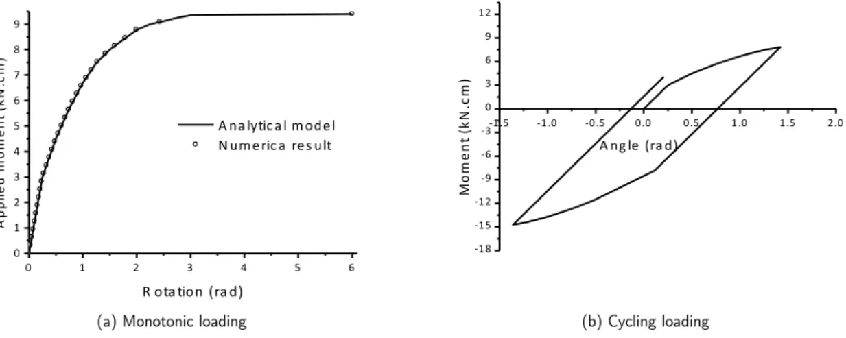
The cross section and the elastic properties of the bar are also depicted in Figure 8. Two finite elements of cubic approximation order have been used and the load is divided into 30 steps. Figure 9a shows the moment versus rotation graphic comparing the numerical result with the analytical curve for a monotonically crescent load. The initial elastic modulus of the connection is

k

=

12 kN .cm

with elastic limit

M

_y

=

3 _{kN .cm}

_{. Figure 9b shows the connection behavior when} subjected to a cyclic loading.

(19)

for example, by Pinheiro and Silveira (2005) and Chan and Chui (2000), the loading situation (Fig-ure 9a) will present the same result as the analytical solution; however their models are unable to reproduce the real unloading or cycling situation (Figure 9b), that is, in their formulation no plastic evolution takes place and the unloading follows the same curve as loading, which results into no plastic residuals at a new resting position.

(a) Monotonic loading (b) Cycling loading

Figure 9 Connection moment x rotation graphics – a) Monotonic, b) Cyclic.

Figure 10 shows partial positions for 15 equally spaced loading levels demonstrating that the non-linear geometric description is exact. This level of rotation is not accomplished by formulations that adopt second order geometrical descriptions.

Figure 10 Partial positions for equally spaced loads

6.2 Four point test

A simple supported beam, subjected to a monotonically crescent controlled displacement at load positions, see Figure 11, is analyzed. The cross section is also presented in Figure 11, for which three lamina are employed to perform the Gauss integration procedure. Five Gauss integration points are adopted for each lamina. Two different materials are employed for comparisons, one is

0 1 2 3 4 5 6

0 1 2 3 4 5 6 7 8 9

A

p

li

e

d

m

o

m

e

n

t

(k

N

.c

m

)

R ota tion (ra d)

A na lytic a l m ode l N um e ric a re s ult

‐1 .5 ‐1 .0 ‐0 .5 0 .0 0 .5 1 .0 1 .5 2 .0

‐1 8 ‐1 5 ‐1 2 ‐9 ‐6 ‐3 0 3 6 9 1 2

Mo

m

e

n

t

(k

N

.c

m

)

A ng le (ra d)

0 4 6

2 12

8 10 14 16 18 20 22 24 26 28

(20)

perfect elastoplastic and the other presents softening, see Figure 12a.

Figure 11 Simple supported beam - loading and cross section

(a) Stress-strain relation (b) Load versus displacement

Figure 12 Curves: stress x strain and force x displacement (under the load)

Figure 12b shows the beam behavior for both materials. Results are compared to the elastic limit load and the ultimate load for perfect elastoplasticity. Position control is sufficient to model the post critical behavior of this example. Three cubic elements (without considering symmetry) are used to model this case.

(a) Perfect elastoplastic (b) Softening

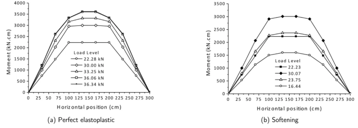
Figure 13 Bending moments diagrams for various load levels

Figure 13 shows the evolution of bending moments for different load levels. One can observe that for the perfect elastoplastic case the degradation spread over the beam; moreover the load stabilizes after the displacement of 7cm. For the material that presents softening, after the imposed

displace-0 2 4 6 8 1 0

0 4 8 1 2 1 6 2 0 S tr e s s ( k N /c m 2 )

S tra in (1 0‐3)

P e rfe c t E la s topla s tic S ofte ning

0 1 2 3 4 5 6 7 8 9

0 4 8 1 2 1 6 2 0 2 4 2 8 3 2 3 6 4 0 L o a d ( k N )

V e rtic a l D is pla c e m e nt (c m ) P e rfe c E la s topla s tic L im it P e rfe c E la s topla s tic ‐ N um e ric a l S ofte ning ‐ N um e ric a l E la s tic L im it

0 2 5 5 0 7 5 1 0 0 1 2 5 1 5 0 1 7 5 2 0 0 2 2 5 2 5 0 2 7 5 3 0 0 0

5 0 0 1 0 0 0 1 5 0 0 2 0 0 0 2 5 0 0 3 0 0 0 3 5 0 0 4 0 0 0

Mo m e n t (k N .c m )

H oriz onta l pos ition (c m )

L oa d L e ve l 2 2 .2 8 k N 3 0 .0 0 k N 3 3 .2 5 k N 3 6 .0 6 k N 3 6 .3 4 k N

0 2 5 5 0 7 5 1 0 0 1 2 5 1 5 0 1 7 5 2 0 0 2 2 5 2 5 0 2 7 5 3 0 0 0

5 0 0 1 0 0 0 1 5 0 0 2 0 0 0 2 5 0 0 3 0 0 0 3 5 0 0

Mo m e n t (k N .c m )

H oriz onta l pos ition (c m )

(21)

ment of 2.2cm a reduction in the load level occurs for crescent imposed displacements and, conse-quently, in the bending moment. Moreover, no bending moment spreads over the beam.

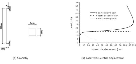
6.3 Elastoplastic column

This example illustrates the application of the proposed formulation to the eccentric compression of the column depicted in Figure 14a. The material properties are:

E

₌

21000

kN / cm

2,

ν

=

0 .

0

_and

σ

y

=

21 kN / cm

2_{with perfect elastoplasticity. Figure 14b shows the results obtained using the}

proposed formulation (geometrically exact) for the elastic and elastoplastic cases. These solutions are compared to the elastic closed second order analytical solution (secant formulae). We adopt six cubic finite elements to run this example, four along the column and two for the small consoles at extremities. Position control is employed and, to impose symmetry, the rotation of the central node is restricted.

(a) Geometry (b) Load versus central displacement

Figure 14 Eccentric column and results.

This example confirms that the elastic second order theory gives a more flexible result than the elastic geometrically exact one. The plastic flow starts at the load level of

13kN

_,

16%

_{less than} the column critical load (

15 .

545 kN

_{). The elastic release starts at the load level}

3 .

773 kN

_{and the}

residual displacement, at the new unloaded situation, is about

30 cm

_.

6.4 Frame analysis subjected to concentrated loads - Elastoplastic connection

In this example the frames depicted in Figure 15 are analyzed considering elastoplastic connections. The original data of this problem are given by Pinheiro and Silveira (2005) and Chan and Chui (2000). In these works the connection model does not consider plasticity, the geometry follows the second order approximation and the kinematic does not include shear effects. To simplify compari-sons, we adopt elastic bars with

E

=

21000kN / cm

2 and

ν

=

0.0

.

The adopted multi-linear connection diagrams, shown in Figure 16, are extracted from Pinheiro and Silveira (2005). The elastic limits of the connections for the four tested cases are:

0 1 0 2 0 3 0 4 0 5 0 6 0 7 0 8 0 9 0 1 0 0 1 1 0 1 2 0 0

5 1 0 1 5 2 0 2 5 3 0 3 5 4 0 4 5 5 0 5 5

L

o

a

d

(

k

N

)

(22)

M

_yA

=

750 _{kN .cm}

_,

_M

y B

=

1625

_{kN .cm}

_,

_M

y C

=

5000

_{kN .cm}

_and

_M

y D

=

20480

_{kN .cm}

_{with their}

corresponding rotations

θ

y A

=

1 _.

67 _x

10

−3

_rad

_,

θ

y B

=

1 _.

67 _x

10

−3

_rad

_,

θ

y C

=

5 _.

00 _x

10

−3

_rad

_and

θ

y D

=

6 _.

67 _x

10

−3

_rad

_{. More data information can be seen in Pinheiro and Silveira (2005).}

Beams are constituted of steel wide flange shaped section

W

14 x

48

while columns are

constitut-ed of

W

12 x

96

section. It is interesting to note that bars behave elastically because the ultimate limit of the strongest connection (case D) is practically equal to the elastic limit of beams, and loads are applied at connections.

The load

_P

(Figure 15) grows monotonically until the critical load shows up. Figures 17 and 18 show that the results presented by our formulation agree with the ones given by references. For semi-rigid connections the differences in results are less the 2% for all cases. For rigid connection the difference is about 6%, explained by the difference among the exact geometrical description and second order approximation.

a) Clamped b) Simple supported

Figure 15 Analized frames, adapted from Pinheiro and Silveira (2005)

Figure 16 Connections bending moment x rotation diagrams

0 .0 0 0 .0 1 0 .0 2 0 .0 3 0 .0 4 0 .0 5 0 .0 6 0 .0 7 0 .0 8 0 .0 9 0 .1 0 0

5 0 0 0 1 0 0 0 0 1 5 0 0 0 2 0 0 0 0 2 5 0 0 0 3 0 0 0 0

Mo

m

e

n

t

(k

N

.c

m

)

A ng le (ra d)

(23)

Figure 17 Simple supported structure behavior

Figure 18 Clamped structure behavior

For connections A and B the displacement levels are very small and failure occurs in an abrupt way. In order to show up the horizontal plateau (for A and B), Figures 17 and 18, we used lateral loads of

0 .

0015

P

_and

0 .

003 P

_{instead of}

0.001P

_and

0 .

002 P

_{. However, this procedure does not}