Spatial and temporal variability in surface ozone at a high elevation remote site in Nepal

(1)

ACPD

9, 16233–16266, 2009

Spatial and temporal variability in surface

ozone in Nepal

G. W. K. Moore et al.

Title Page

Abstract Introduction

Conclusions References

Tables Figures

◭ ◮

Back Close

Full Screen / Esc

Printer-friendly Version

Interactive Discussion

Atmos. Chem. Phys. Discuss., 9, 16233–16266, 2009 www.atmos-chem-phys-discuss.net/9/16233/2009/ © Author(s) 2009. This work is distributed under the Creative Commons Attribution 3.0 License.

Atmospheric Chemistry and Physics Discussions

This discussion paper is/has been under review for the journalAtmospheric Chemistry

and Physics (ACP). Please refer to the corresponding final paper inACPif available.

Spatial and temporal variability in surface

ozone at a high elevation remote site in

Nepal

G. W. K. Moore1, S. Abernethy1, and J. L. Semple2

1

Department of Physics, University of Toronto, Toronto, Canada

2

Department of Surgery, University of Toronto, Toronto, Canada

Received: 9 July 2009 – Accepted: 20 July 2009 – Published: 29 July 2009

Correspondence to: G. W. K. Moore ([email protected])

(2)

ACPD

9, 16233–16266, 2009

ozone in Nepal

Title Page

Tables Figures

◭ ◮

Back Close

Full Screen / Esc

Abstract

Ozone is an important atmospheric constituent due to its role as both a greenhouse gas and an oxidant. Recent measurements in the Mount Everest region indicate the

presence of ozone at elevations from 5000 to 9000 m a.s.l.that are the result of both

stratospheric and tropospheric sources. Here we examine the temporal variability in

5

the surface ozone concentration measurements from the ABC-Pyramid Observatory in the Mount Everest region during 2006 and compare it to the total column ozone data from the OMI instrument as well as meteorological fields from the ECMWF Interim Re-analysis. Both the surface ozone at and the total column ozone over the ABC-Pyramid Observatory site have maxima in the pre-monsoon period. We show that during this

10

period, there is a statistically significant correlation between the two suggesting that the stratosphere was an important contributor to the high levels of ozone observed during the period. There was a hiatus in the monsoon in June that resulted in a return of westerlies over northern Indian and southern Tibet and as a result, the aforemen-tioned correlation extended into June. No such correlation exists during the monsoon

15

and post-monsoon periods. Spatial correlation maps between the surface ozone and total column ozone as well as meteorological fields from the ECMWF Interim Reanal-ysis support the contention that there is a significant stratospheric contribution in the pre-monsoon period that is absent during and after the monsoon.

1 Introduction

20

Ozone is an important atmospheric constituent as a result of its role as a greenhouse gas (Fishman et al., 1979; Ramanathan and Feng, 2009) and as an active oxidant that has been associated with a range of health outcomes (Burnett et al., 1997) as well as inhibiting plant growth (Manning et al., 1996). Tropospheric ozone has two sources: the photochemical production within the troposphere and the downward transport from

25

(3)

ACPD

9, 16233–16266, 2009

ozone in Nepal

Title Page

Tables Figures

◭ ◮

Back Close

Full Screen / Esc

varies seasonally as well as with location. Industrialized regions in the Northern Hemi-sphere typically experience a broad summertime maximum that are the result of photo-chemical production (Logan, 1985), while remote areas typically experience a spring-time maximum (Davies and Schuepbach, 1994). The limited measurements that are available from the late 19th century also show a springtime maximum (Bojkov, 1986).

5

The reasons for this springtime maximum are still unclear (Monks, 2000), although stratosphere/troposphere exchange is thought to play a role (Logan, 1985; Davies and Schuepbach, 1994).

Starting with the work of Dobson and collaborators (Dobson and Harrison, 1926; Dobson et al., 1927), variability in total column ozone (TCO) has been shown to be

10

associated with surface pressure and other meteorological variables. In particular, Dobson and Harrison (1926) showed that high values of TCO were associated with low surface pressure; with low values of TCO being associated with high surface pressure. They furthermore noted that because much of the ozone is situated in the stratosphere, this correlation was presumably the result of a relationship between these fields in the

15

stratosphere that was expressed at the surface. Aircraft observations in conjunction with space based measurements of TCO by the Total Ozone Mapping Spectrometer (TOMS) family of instruments (McPeters, 1998) have shown that gradients in the TCO field are usually associated with intrusions, known as tropopause folds, of ozone-rich stratospheric air into the upper-troposphere that often have as their surface expression,

20

a region of low pressure (Danielsen, 1968; Shapiro, 1980; Goering et al., 2001; Hudson et al., 2003).

On occasion, these folds have been sufficiently deep as to result in elevated levels

of ozone at the earth’s surface (Lamb, 1977; Davies and Schuepbach, 1994). The elevated levels of ozone in these folds are diluted through mixing as they descend

25

(4)

moun-ACPD

9, 16233–16266, 2009

ozone in Nepal

Title Page

Tables Figures

◭ ◮

Back Close

Full Screen / Esc

tainous regions (Reiter et al., 1977; Stohl et al., 2003). Ozone levels throughout the troposphere are increasing at many locations and are expected to continue to increase throughout the 21st century as a result of population growth and an increase in fossil fuel use (Logan et al., 1999; Houghton, 2001). This is especially true over the In-dian subcontinent where surface ozone concentrations are predicted to increase by as

5

much as 10% by 2030 (Dentener et al., 2006).

The Himalaya are therefore an important region in which to study surface ozone and its sources given that it is adjacent to the rapidly industrializing Indian subcontinent with its increasing concentration of tropospheric ozone as well as being a region of extremely high topography that increases the influence of stratospheric ozone. From

10

a meteorological perspective, it is at a lower latitude as compared to the Alps, the mountainous region where surface ozone has been most extensively studied, and so falls under the influence of the subtropical jet and monsoonal circulations whose impact on surface ozone has not been extensively studied.

With respect to the Himalaya, Moore and Semple (2004, 2006) reported that high

15

impact weather events on Mount Everest are often associated with the passage of tropopause folds. They hypothesized that these folds would have resulted in high ozone concentration near that summit that could have an impact on climbers. Moore and Semple (2005) reported on surface ozone measurements from 5000 m above sea level (a.s.l.) in the Bhutanese Himalaya that indicated an increase in ozone with height

20

that was associated with the passage of a tropopause fold. Observations in Tibet,

near Mount Everest, recorded a diurnal pattern in ozone concentration at 5000 m a.s.l.

with maxima at night that was attributed to the transport of stratospheric ozone by thermally driven valley circulations (Zhu et al., 2006). During May 2005, surface ozone concentration measurements were made at elevations near and at the summit of Mount

25

(5)

ACPD

9, 16233–16266, 2009

ozone in Nepal

Title Page

Tables Figures

◭ ◮

Back Close

Full Screen / Esc

2900 to 5200 m a.s.l.during April 2007. Along this transect, they observed an increase

in ozone exposure with height with a maximum 8-h exposure in excess of 140 ppb. These elevated levels were in excess of World Health Organization guidelines and were shown to be the result of the passage of a tropopause fold over the region (Moore and Semple, 2009). Moore and Semple (2009) estimated that these events occur

5

approximately 10% of the time in April.

Surface ozone concentration measurements at the ABC-Pyramid Observatory

lo-cated approximately 20 km south of Mount Everest at an elevation of 5079 m a.s.l.

were initiated in March 2006 (Bonasoni et al., 2008) and show evidence of a springtime maximum during which were many relatively short events in which the

stratospheric-10

troposphere exchange was found, through the analysis of back-trajectories, to be source of the elevated levels of ozone observed. These events were also found to be associated with clean and dry air masses. During mid-June 2006, there was a pe-riod of approximately 10 days in which elevated levels of ozone were observed. This event was argued to be the result of the transport of a polluted air mass from the Indus

15

Valley to the site (Bonasoni et al., 2008).

In subsequent work, Cristofanelli et al. (2009) developed an algorithm that uses the surface ozone concentration and pressure measurements at the ABC-Pyramid Ob-servatory along with back-trajectories and TCO values to identify events in there was a significant transport of ozone-rich stratospheric air into the upper troposphere. These

20

events occurred approximately 10% of the time with a pronounced minimum during the monsoon period (Cristofanelli et al., 2009).

The results present in Bonasoni et al. (2008) and Cristofanelli et al. (2009) clearly suggest that there is a transition in the role that the stratospheric source plays in sur-face ozone levels in the Mount Everest region. This is consistent with the results of

25

(6)

ACPD

9, 16233–16266, 2009

ozone in Nepal

Title Page

Tables Figures

◭ ◮

Back Close

Full Screen / Esc

associated with the transport of polluted tropospheric air from South-East Asia into the region.

The monsoon onset over Kerala (MOK) is the standard metric used to identify the start of the Indian summer monsoon (Pai and Nair, 2009). For the period from 1971– 2007, the average date of the MOK was 1 June with a standard deviation of 8 days

5

(Pai and Nair, 2009). In 2006, the MOK occurred on 26 May. Typically the monsoon arrives in the Mount Everest region approximately 10–15 days after the MOK (Soman and Kumar, 1993). However 2006 was an anomalous year in which there was a hiatus in the progression of the monsoon from 7 June to 22 June that resulted from the re-establishment of mid-latitude westerlies over the region. As a result in 2006, the arrival

10

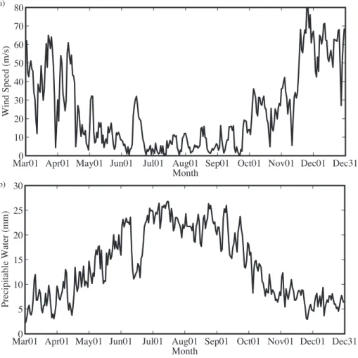
of the monsoon over the Mount Everest region occurred around 27 June (Jayanthi et al., 2006). Figure 1 shows the 300 mb horizontal wind speed and precipitable water, total column water vapour, over the ABC-Pyramid Observatory site for the period 1 March to 31 December 2006. The reduction in wind speed and increase in precipitable water that occurred in late April and May is indicative of the northward movement of the

15

sub-tropical jet that presages the onset of the monsoon. The extended period of high wind speeds and low precipitable water in mid June was associated with the hiatus

in the onset of the monsoon. Please note that this definition differs from that used

by Bonasoni et al. (2008) and Cristofanelli et al. (2009) who used local conditions at the ABC-Pyramid Observatory site, in particular high relative humidity and night-time

20

southerly winds, to identify the onset of the monsoon. With these criteria, the monsoon was deemed to have arrived on 21 May – approximately 5 weeks prior to the synoptic-scale onset date.

In this paper, we will explore the temporal and spatial relationship between the sur-face ozone concentration measured at the ABC-Pyramid Observatory with TCO values

25

(7)

ACPD

9, 16233–16266, 2009

ozone in Nepal

Title Page

Tables Figures

◭ ◮

Back Close

Full Screen / Esc

2 Data and methods

Surface ozone concentration measurements at the ABC-Pyramid Observatory

(27◦57′N; 86◦48′E; 5079 m a.s.l.) were begun in March 2006 using a UV-photometric

analyser (Bonasoni et al., 2008). Data is available every 30 min and for this paper, we have used the data at noon local time for the period 1 March to 31 December 2006.

5

For further information, please refer to Bonasoni et al. (2008).

The total column ozone as measured by the space-based TOMS instrument, and its successor the OMI instrument, provides a succinct dataset with which to identify intru-sions of stratospheric air into the upper-troposphere (Hudson et al., 2003). These in-struments provide measurements of total column ozone at local solar noon (McPeters

10

and coauthors, 1998; Levelt et al., 2006). For this paper, we have used the level 3

gridded product that is available at a horizontal resolution of 1◦. The TOMS data has

been used in a number of studies in the Mount Everest region to identify tropopause folds and the concomitant intrusions of ozone-rich stratosphere air into the upper tro-posphere (Moore and Semple, 2004, 2005, 2006; Cristofanelli et al., 2009; Moore and

15

Semple, 2009).

Beginning in 1999, stratospheric ozone data has been assimilated into the ECMWF’s operational analysis and reanalyses in order to improve the use of satellite radiances as well as to infer information on the wind field in the vicinity of the tropopause (Dethof and Holm, 2004). In a comparison with independent data from the UARS satellite and

in-20

strumented MOZAIC aircraft, the ERA-40 reanalysis was found to overestimate ozone in the lower stratosphere and upper-troposphere by 5–10% (Oikonomou and O’Neill, 2006). The ERA-I is a new reanalysis product developed by the European Center for Medium-Range Weather Forecasts (ECMWF) that is at a higher horizontal resolution with additional vertical levels as compared to older global reanalysis products

(Sim-25

(8)

ACPD

9, 16233–16266, 2009

ozone in Nepal

Title Page

Tables Figures

◭ ◮

Back Close

Full Screen / Esc

on isentropic surfaces from the ERA-I to diagnose the source of the high ozone con-centrations that were observed along the Khumbu Valley.

3 Results

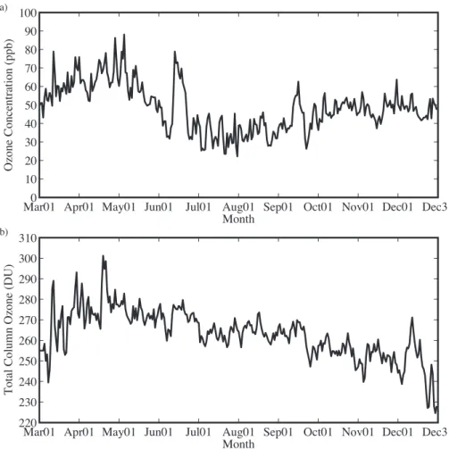
Figure 2 shows the time series of surface ozone concentration at local noon from the ABC-Pyramid Observatory for the period 1 March to 31 December 2006. Also shown

5

is the time series of TCO over the site extracted from the L3 gridded data. Both time series attain their highest values in April with multiple instances of maxima of a short duration during this period. The surface ozone concentration time series shows a pro-nounced drop in magnitude during May with an extended period of elevated values in mid June. Comparison with Fig. 1 shows that this event in June occurred during the

10

hiatus in the onset of the monsoon when there was a return of westerlies and a reduc-tion in precipitable water over the region. Subsequently the concentrareduc-tion remained low during July and August before recovering later in the year. Throughout this period there were also isolated maxima. The TCO time series shows a more gradual decline after April with the lowest values occurring near the end of the year.

15

A comparison of the two time series shows a degree of correlation with a num-ber of events in which both the surface ozone concentration and the TCO were ele-vated. However, the relative magnitude of the values during these events was often uncorrelated. For example, the highest TCO was observed on 19 April. There was a corresponding local maxima in surface ozone concentration, although the highest

20

concentration was recorded on 5 May. The elevated period of high surface ozone con-centration in early June was also a period in which the TCO was elevated. For the entire period under consideration, the correlation between the two time series was 0.39. The statistical significance of this correlation was determined using a resampling technique that that made use of 1000 synthetic time series constructed to have the same power

25

(9)

ACPD

9, 16233–16266, 2009

ozone in Nepal

Title Page

Tables Figures

◭ ◮

Back Close

Full Screen / Esc

correlation between the two time series was determined to be 87%.

Both time series shown in Fig. 2 clearly exhibit a change in behavior during the period

under consideration. This suggests that there may be some differences in the nature

of the correlation throughout the year as one moves from the pre-monsoon period through the monsoon period and into the post-monsoon period. This is consistent

5

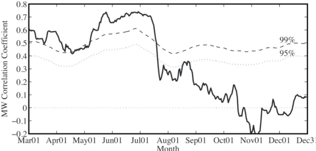
with the finding of Cristofanelli et al. (2009) who found a pronounced minima in the stratospheric contribution to surface ozone concentration during the monsoon period. To assess this non-stationarity in the correlation between the two time series, a moving window correlation was performed. A 60 day window length was chosen so as to capture the seasonal change in the nature of the correlation between the two time

10

series. Similar results were obtained with other seasonal-scale window lengths. The results are presented in Fig. 3. Significance levels obtained with the same resampling technique described above are indicated. For windows centered on dates from start of

March through to the end of June, the correlation coefficient was on the order of 0.6

and was significant at the 99% level. After the start of July, there was a dramatic drop in

15

the correlation coefficient to statistically insignificant levels on the order of 0.2. Starting

in October, the magnitude of the correlation dropped further with a period in November in which it was actually negative.

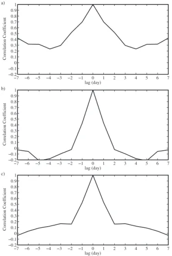
To provide information on the temporal characteristics of the surface ozone con-centration at the ABC-Pyramid Observatory, we show in Fig. 4 the autocorrelation of

20

this time series for three di_fferent periods: 1 April–30 June; 1 July–30 September and

1 October–31 December. These periods are meant to roughly correspond to the pre-monsoon, the monsoon and the post-monsoon conditions during 2006 as identified in Fig. 3. During the pre-monsoon period, (Fig. 4a), there was a broad peak to the au-tocorrelation with evidence of secondary maxima on the time scale of one week. In

25

contrast during the monsoon period (Fig. 4b), there was a narrow peak to the autocor-relation with values rapidly dropping to close to zero. During the post-monsoon period

(Fig. 4c), there was again a narrow peak but with a reduction in the rate of drop-off

(10)

ACPD

9, 16233–16266, 2009

ozone in Nepal

Title Page

Tables Figures

◭ ◮

Back Close

Full Screen / Esc

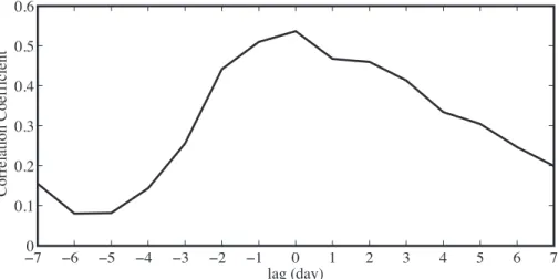
Given the high degree of correlation between the surface ozone concentration at the ABC-Pyramid Observatory and TCO over the site during the pre-monsoon period, we show in Fig. 5 the lagged autocorrelation between the two time series for the period 1 April–30 June. The lagged autocorrelation is asymmetric with a rapid increase for

negative lags and a much slower drop-off for positive lags. That is; there was little or

5

no correlation between the two time series during the days leading up to a high ozone event at the ABC-Pyramid Observatory site, while after the event TCO remained high for a number of days.

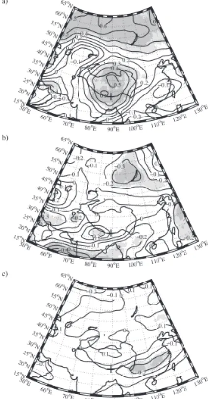
To provide information on the spatial pattern of the correlation or lack therof, spa-tial correlation maps between the surface ozone concentration at the ABC-Pyramid

10

Observatory and TCO throughout the South-East and Central Asia were calculated for the three periods described above. The results are presented in Fig. 6 along with measures of the statistical significance of the correlation based on the resampling tech-nique described above. During the period 1 April–30 June, there was a region of high and statistically significant correlation centered over Tibet as well as a second region

15

north of 55◦N. During the other two periods, the situation was quite different with small

and scattered regions of statistical significance of both signs. Of most relevance to the present study is the small region of statistically significant positive correlation during the period 1 July–30 September located just to the west of the ABC-Pyramid Observatory site.

20

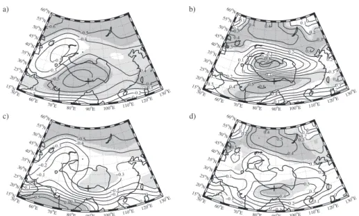
Figure 7 shows the spatial correlation maps between the surface ozone concentra-tion at the ABC-Pyramid Observatory and the geopotential height and the horizontal wind fields from the ERA-I on the 300 mb and 500 mb pressure surfaces for the period 1 April–30 June. Also shown are measures of the statistical significance of the correla-tions based on the resampling technique described above. At 300 mb, the geopotential

25

height correlation was negative and statistically significant throughout much of the do-main of interest with the exception of a region to the northwest of Tibetan Plateau to the east of the Caspian Sea. As was the case with the TCO map (Fig. 4a), the magnitude

(11)

ACPD

9, 16233–16266, 2009

ozone in Nepal

Title Page

Tables Figures

◭ ◮

Back Close

Full Screen / Esc

The 300 mb wind speed correlation map had a statistically significant tripolar structure with a region of positive correlation to the south and north of the plateau with a region of negative correlation over the plateau itself. At 500 mb, the structure of the correla-tion maps were similar to those at 300 mb with the excepcorrela-tion that the magnitudes of the correlations were generally reduced. In addition, there was a region of positive and

5

statistically significant correlation with the geopotential height over southern India, the Arabian Sea and parts of the Bay of Bengal.

Figure 8 shows the same spatial correlation maps except for the period 1 July– 30 September. In general, the magnitude and spatial extent of the statistically signifi-cant correlations were reduced as compared to the pre-monsoon period (Fig. 7a). At

10

300 mb, there was however still a region of negative correlation with the geopotential height field over the Tibetan Plateau. At 500 mb, the region of negative correlation with the geopotential height over the plateau was not present. With respect to the wind speed, there was at 300 mb a dipolar pattern of statistically significant correlation that bracketed the ABC-Pryamid Observatory site.

15

Figure 9 shows the same spatial correlation maps except for the period 1 October– 31 December. At both 300 mb and 500 mb, there was an elongated region, extending from northwest India across the Tibetan Plateau to Lake Baikal in Siberia, of statisti-cally significant negative correlation with the geopotential height field as well as local-ized regions near the ABC-Pyramid Observatory site where there were positive and

20

statistically significant correlations with the horizontal wind speed.

Motion in the upper-troposphere and lower-stratosphere, is quasi-adiabatic and therefore occurs, to first order, along surfaces of constant potential temperature (Hoskins, 1991). All potential temperature surfaces slope upwards as one moves polewards in the Northern Hemisphere with the 330 K surface typically situated in

25

(12)

ACPD

9, 16233–16266, 2009

ozone in Nepal

Title Page

Tables Figures

◭ ◮

Back Close

Full Screen / Esc

have also therefore considered correlation maps with potential vorticity and ozone con-centration on these surfaces. Potential vorticity is a relatively simple and widely used diagnostic that allows one to distinguish between air of tropospheric and stratospheric

origin with values in the range of 1 to 2 PV units (1 PVU=10−6K s−2kg−1) usually

serv-ing as the cut-o_ff(Hoskins, 1991).

5

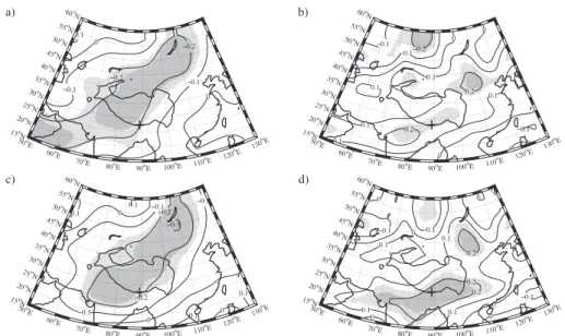
Figure 10 shows the spatial correlation maps between the surface ozone tion at the ABC-Pyramid Observatory and the potential vorticity and ozone concentra-tion on the 330 K and 350 K isentropic surfaces for the period 1 April–30 June. Also shown are measures of the statistical significance of the correlations based on the re-sampling technique described above. The correlation maps at 330 K indicate a positive

10

and statistically significant correlation in the fields over the Tibetan Plateau as well as

to the north of 55◦N. At 350 K, the correlations are similar although there was a larger

area of positive correlation.

Figures 11 and 12 show the same spatial correlation maps except for the periods 1 July–30 September and 1 October–31 December. Unlike the correlation maps shown

15

in Fig. 10, the correlations were smaller in magnitude as well as in the area of statistical significance and as a result, no coherent pattern emerges.

4 Discussion

The results presented in this paper support the contention that there is a seasonality in the temporal characteristics as well as the source region for the surface ozone

ob-20

served at the ABC-Pyramid Observatory. The year under investigation, 2006, was an anomalous one in which there was a hiatus in the monsoon during June (Fig. 1) that resulted in a delay in the onset of the monsoon over the Mount Everest region until late June.

At the ABC-Pyramid Observatory site, the surface ozone values were highest during

25

(13)

ACPD

9, 16233–16266, 2009

ozone in Nepal

Title Page

Tables Figures

◭ ◮

Back Close

Full Screen / Esc

duration events in which the ozone value was elevated. The hiatus in the monsoon in June coincided with a return of high ozone values at the site. The TCO is a proxy for the presence of tropopause folds and its time series over the site also had a maximum during the pre-monsoon period (Fig. 2b). Throughout the rest of the year, there was a trend towards lower values of TCO. Many of the high ozone events at the

ABC-5

Pyramid Observatory site coincided with high TCO values, although there appeared to be no simple relationship between the relative magnitudes of the quantities during these events. Unlike what occurred for the surface ozone time series, the TCO did not show any recovery to higher values during the post-monsoon period.

Over the entire period under investigation, 1 March to 31 December 2006, the

cor-10

relation between the two time series was not statistically significant at the 95% level. However, a moving window correlation (Fig. 3) indicated that the correlation between

the two time series was different during the pre-monsoon, monsoon and post-monsoon

periods. During the pre-monsoon period, the correlation was high and statistically sig-nificant at the 99% levels. The onset of the monsoon resulted in a sharp drop in the

15

magnitude of the correlation, while during the post-monsoon period there was a further reduction in magnitude and even a period in which the correlation was negative. This non-stationarity resulted in the low correlation between the two time series over the entire period.

The autocorrelation of the surface ozone time series provides information on the

20

nature of the observed maxima (Fig. 4). During the pre-monsoon period, the autocor-relation had a broad peak as well as evidence of secondary maxima on time scales of one week that suggests a periodicity on this time scale in the underlying time series. During the monsoon and post-monsoon periods, the peak in the autocorrelation was much narrower with a much reduced evidence of secondary maxima. This suggests

25

that during these periods, the high ozone events were temporally uncorrelated. This lack of temporal autocorrelation was highest during the monsoon period.

(14)

ACPD

9, 16233–16266, 2009

ozone in Nepal

Title Page

Tables Figures

◭ ◮

Back Close

Full Screen / Esc

between the two during the pre-monsoon period (Fig. 5). In particular, it has an asym-metrical shape with a sharp rise for negative lags and a broader descent for positive lags. This suggests that in the days prior to a high ozone event at the ABC-Pyramid Observatory site, there are not corresponding high values of TCO over the site, while after the high ozone event TCO values remained elevated over the site for a number of

5

days.

Spatial correlation maps between surface ozone at the ABC-Pyramid Observatory and TCO show clear evidence of a synoptic-scale, coherent and statistically significant distribution during the pre-monsoon period (Fig. 6a) with a maximum over the Tibetan Plateau as well as to the north of the plateau. This pattern is reminiscent of what is

10

observed during tropopause fold events over the region that resulted in high surface ozone events in the region (Semple and Moore, 2008; Moore and Semple, 2009) in which a filament of high TCO extended southwards from high latitudes towards the Mount Everest region. The lack of correlation in the region immediately to the north of

the plateau is most likely the result of differences in the position of the filament between

15

the various events. Please note that the maximum over the plateau is upwind of the Mount Everest region. This implies that in the days prior to a high ozone event, there would tend to be no corresponding high TCO values over the site. In contrast, after an event the TCO would remain high as the remainder of the fold passed over the site. This behaviour is consistent with the lagged correlation noted in Fig. 5. Tropopause folds

20

tend to associated with the passage of upper-level Rossby waves that have a periodicity on the order of one week (Palm ´en and Newton, 1969) and as a result, one would expect to see a periodicity in the high ozone events in the pre-monsoon period. This is consistent with the autocorrelation in the surface ozone (Fig. 4a) as well as that the TCO over the ABC-Pyramid site (not shown) during the pre-monsoon period.

25

(15)

ACPD

9, 16233–16266, 2009

ozone in Nepal

Title Page

Tables Figures

◭ ◮

Back Close

Full Screen / Esc

stratosphere that is consistent with the results of Cristofanelli et al. (2009) who found that even during the monsoon period, there was a contribution from the stratosphere to surface ozone at the ABC-Pyramid Observatory site, or it may be the result of a residual signal of tropopheric ozone in the TCO (Ziemke et al., 2006). The picture was similar during the post-monsoon period (Fig. 6c).

5

The spatial correlation maps between surface ozone at the ABC-Pyramid Observa-tory and the geopotential height and horizontal wind speed fields on the 300 mb and 500 mb levels from the ERA-I are consistent with the results discussed above. In par-ticular during the pre-monsoon period, there is a negative correlation between surface ozone at the ABC-Pyramid Observatory site and 300 mb geopotential height over the

10

Tibetan Plateau as well as a positive correlation with the wind speed to the south and north of the plateau (Fig. 7a and b). The correlations were similar at 500 mb but smaller in magnitude (Fig. 7c and d). This suggests that high ozone at the site is associated with an upper-tropospheric region of low pressure and an enhancement in the strength of both the sub-tropical and mid-latitude jet streams.

15

During the monsoon and post-monsoon periods, the spatial extent of the correlations is much more muted with the most significant finding being that during both of these periods, there was a negative correlation with the 300 mb geopotential height over the plateau (Figs. 8 and 9). During the monsoon period, there tended to be an anti-cyclone over the plateau and so this finding suggests that high surface ozone events at

20

the ABC-Pyramid Observatory site are associated with a weaker monsoon flow. This result is consistent with the positive correlation with the 500 mb geopotential height (Fig. 8c) and the negative correlation with precipitable water (not shown) over north and central India. It is also consistent with the elevated levels of surface ozone during the June hiatus in the monsoon (Figs. 1 and 2).

25

(16)

ACPD

9, 16233–16266, 2009

ozone in Nepal

Title Page

Tables Figures

◭ ◮

Back Close

Full Screen / Esc

correlations were present on the 350 K surface. These results are again consistent with the presence of a tropopause fold during high ozone events at the ABC-Pyramid Observatory during the pre-monsoon period and a significant stratospheric contribution to these events. As was the case for the TCO and isobaric correlation maps, there was no corresponding upper-tropospheric feature present during monsoon and

post-5

monsoon high ozone events.

5 Conclusions

In this paper, we have examined the temporal characteristics of the surface ozone concentration observed at the ABC-Pyramid Observatory site during 2006 and its re-lationship to stratospheric ozone and the synoptic-scale flow. Given the proximity to

10

the Indian subcontinent, the site is clearly under the influence of monsoonal flow with strong westerlies associated with the sub-tropical jet stream present during the pre and post monsoon period and the Tibetan anti-cyclone and the Indian monsoon trough dur-ing the monsoon period. Surface ozone at the site attains its highest values durdur-ing the pre-monsoon period. During this period, there is evidence of temporal autocorrelation

15

that suggests that maxima are associated with synoptic-scale phenomenon. During the monsoon period, the temporal autocorrelation is much weaker suggesting that the maxima are isolated events. The post-monsoon period represents a mixing of these two behaviors with some evidence of temporal autocorrelation.

The correlation between the surface ozone concentration observed at the site and

20

TCO over the site, a widely recognized proxy for the presence of tropopause folds, varies throughout the year with a high degree of correlation during the pre-monsoon period and much lower degrees of correlation during the monsoon and post-monsoon periods. This suggests, in agreement with previous studies (Moore and Semple, 2004, 2005, 2006; Bonasoni et al., 2008; Cristofanelli et al., 2009; Moore and Semple, 2009),

25

(17)

ACPD

9, 16233–16266, 2009

ozone in Nepal

Title Page

Tables Figures

◭ ◮

Back Close

Full Screen / Esc

a sharp leading edge (Danielsen, 1968; Shapiro, 1980). The lagged correlation be-tween surface ozone at the site and TCO over the site during the pre-monsoon period is consistent with this characteristic in that there was no evidence of a correlation be-tween the two in the days leading up to a high ozone event at the site and a persistence to the correlation after an event.

5

Spatial correlation maps with meteorological fields on both isobaric and isentropic surfaces during the pre-monsoon period are consistent with a synoptic-scale strato-spheric source. In particular, high ozone at the site was associated with low pressures at 300 mb over and to the north of the Tibetan Plateau as well as an increase in the strength of the sub-tropical and mid-latitude jet streams. In addition, higher values of

10

potential vorticity and ozone concentration on the 330 K isentropic surface suggests that a descent of the tropopause was occurring during these events. The spatial phasing of these synoptic-scale features was consistent with the lagged correlation observed between surface ozone at the site and TCO.

There was no evidence of coherent synoptic-scale correlations between surface

15

ozone at the site and TCO and meteorological fields during monsoon periods. The exception being that during this high ozone at the site was associated with lower geopo-tential heights over Tibet. This suggests, as was found by Cristofanelli et al. (2009), that the stratospheric contribution is reduced during the monsoon period. The lack of any coherent synoptic-scale flow associated with high ozone events during the monsoon

20

period suggests that there are a number of pathways by which tropospheric ozone can reach the site. It is consistent with the autocorrelation results which suggest that events during this period are temporally uncorrelated.

The results presented here for the post-monsoon period are similar to those during the monsoon period and suggest that the stratospheric contribution is small. The TCO

25

(18)

ACPD

9, 16233–16266, 2009

ozone in Nepal

Title Page

Tables Figures

◭ ◮

Back Close

Full Screen / Esc

site during the post-monsoon period do not show evidence of the presence of well-developed tropopause folds. Clearly, this period is one in which further research is needed to identify the source of high surface ozone.

As discussed, 2006 was an anomalous year in which there was a hiatus in the mon-soon over India in June that was the result of the re-establishment of upper-level

west-5

erlies over the region. This hiatus coincided with a return of high surface ozone values at the ABC-Pyramid site. Bonasoni et al. (2008) argued that this event was associated with the transport of polluted air from the Indus Valley. Based on the results presented in this paper, it cannot be excluded that there was a stratospheric contribution as well. Based on 8 years of data, the surface ozone concentraton during June in the Indus

Val-10

ley is 25±12 ppb with a maximum observed concentration of 63 ppb (Naja et al., 2003).

It was clear that the concentrations observed at the ABC-Pyramid Observatory during this event, in excess of 60 ppb, cannot be soley the result of the transport of polluted air

from this region. However, thejuxtaposition of both a tropospheric and stratospheric

source would explain the very high values observed during this event.

15

It is clear that the variability in surface ozone at the ABC-Pyramid Observatory is associated with synoptic-scale flow over the extended region that includes much of south-east and central Asia. As such, it may be more approriate to use large-scale measures of the onset, and by inference the cessation, of the monsoon to characterize the variablity in surface ozone at the site and its source region. Such an approach may

20

improve the results obatained by Cristofanelli et al. (2009) as would a change in their algorithim to include only negative synoptic-scale pressure anomalies over the Tibetan Plateau, a robust signature of high ozone events during the pre-monsoon, monsoon and post-monsoon periods.

Finally, the surface ozone concentrations observed at the ABC-Pyramid Observatory

25

(19)

ACPD

9, 16233–16266, 2009

ozone in Nepal

Title Page

Tables Figures

◭ ◮

Back Close

Full Screen / Esc

with the assumption, built into most epidemological models relating health outcomes to pollution, that outdoor air pollution is not a risk factor for rural populations in less-developed countries (Peabody et al., 2005; Semple and Moore, 2009). It also follows that increasing levels of air pollution in southeast Asia pose not only a risk to the cli-mate (Ramanathan et al., 2007) but also to the health of populations in remote regions

5

of the Himalaya.

Acknowledgements. The authors would like to thank P. Bonasoni for providing access to the

ABC-Pyramid Observatory data. The OMI TCO data was provided by NASA, while the ERA-I data was provided by the ECMWF. GWKM was supported by the Natural Sciences and Engi-neering Research Council of Canada.

10

References

Bojkov, R. D.: Surface ozone during the 2nd-half of the 19th-century, J. Clim. Appl. Meteorol., 25 (3), 343–352, 1986.

Bonasoni, P., Lag, P., Angelini, F., et al.: The ABC-Pyramid Atmospheric Research Observatory in Himalaya for aerosol, ozone and halocarbon measurements, Sci. Total Environ., 391(2–3),

15

252–261, 2008.

Burnett, R. T., Brook, J. R., Yung, W. T., et al.: Association between ozone and hospitalization for respiratory diseases in 16 Canadian cities, Environ. Res., 72(1), 24–31, 1997.

Cristofanelli, P., Bonasoni, P., Bonafe, U., et al.: Influence of lower stratosphere/upper tro-posphere (LS/UT) transport events on surface ozone at the Everest-Pyramid GAW Station

20

(Nepal, 5079 m a.s.l.): first year of analysis, Int. J. Remote Sens., in press, 2009.

Danielsen, E. F.: Stratospheric-tropospheric exchange based on radioactivity ozone and po-tential vorticity, J. Atmos. Sci., 25(3), 502–518, 1968.

Davies, T. D. and Schuepbach, E.: Episodes of high ozone concentrations at the earths surface resulting from transport down from the upper troposphere lower stratosphere – a review and

25

case-studies, Atmos. Environ., 28(1), 53–68, 1994.

(20)

ACPD

9, 16233–16266, 2009

ozone in Nepal

Title Page

Tables Figures

◭ ◮

Back Close

Full Screen / Esc

Dethof, A. and Holm, E. V.: Ozone assimilation in the ERA-40 reanalysis project, Q. J. Roy. Meteorol. Soc., 130(603), 2851–2872, 2004.

Dobson, G. M. B. and Harrison, D. N.: Measurements of the amount of ozone in the earth’s atmosphere and its relation to other geophysical conditions, Proc. R. Soc. Lon. Ser.-A, 110(756), 660–693, 1926.

5

Dobson, G. M. B., Harrison, D. N., and Lawrence, J.: Measurements of the amount of ozone in the earth’s atmosphere and its relation to other geophysical conditions. Pt. II, Proc. R. Soc. Lon. Ser.-A, 114(768), 521–541, 1927.

Fishman, J., Ramanathan, V., Crutzen, P. J., and Liu, S. C.: Tropospheric ozone and climate, Nature, 282(5741), 818–820, 1979.

10

Goering, M. A., Gallus, W. A., Olsen, M. A., and Stanford, J. L.: Role of stratospheric air in a severe weather event: Analysis of potential vorticity and total ozone, J. Geophys. Res., 106(D11), 11813–11823, 2001.

Hoskins, B. J.: Towards a PV-Theta view of the general-circulation, Tellus A, 4(4), 27–35, 1991. Houghton, J. T.: Climate change 2001: The scientific basis: Contribution of Working Group I to

15

the third assessment report of the Intergovernmental Panel on Climate Change, x, 881 pp., Cambridge University Press, Cambridge, New York, 2001.

Hudson, R. D., Frolov, A. D., Andrade, M. F., and Follette, M. B.: The total ozone field seperated into meteorological regimes, Part I: Defining the regimes, J. Atmos. Sci., 60, 1669–1677, 2003.

20

Jayanthi, N., Rejeevan, M., Srivastave, A. K., et al.: Monsoon 2006 – A Report, IMD Mono-graph, Indian Meteorological Department, 2006.

Lamb, R. G.: Case-study of stratospheric ozone affecting ground-level oxidant concentrations,

J. Appl. Meteorol., 16(8), 780–794, 1977.

Levelt, P. F., Van den Oord, G. H. J., Dobber, M. R., et al.: The ozone monitoring instrument,

25

IEEE T. Geosci. Remote, 44(5), 1093–1101, 2006.

Logan, J. A.: Tropospheric ozone – seasonal behavior, trends, and anthropogenic influence, J. Geophys. Res.-Atmos., 90(ND6), 10463–10482, 1985.

Logan, J. A., Megretskaia, I. A., Miller, A. J., et al.: Trends in the vertical distribution of ozone: A comparison of two analyses of ozonesonde data, J. Geophys. Res.-Atmos., 104(D21),

30

26373–26399, 1999.

Manning, W. J., Krupa, S. V., Bergweiler, C. J., and Nelson, K. I.: Ambient ozone (O₃) in

(21)

ACPD

9, 16233–16266, 2009

ozone in Nepal

Title Page

Tables Figures

◭ ◮

Back Close

Full Screen / Esc

samplers, Environ. Pollut., 91(3), 399–403, 1996.

McPeters, R. D., Bhartia, P. K., Krueger, A., et al.: Earth Probe Total Ozone Mapping Spec-trometer (TOMS) data products user’s guide, 70 pp., NASA, 1998.

Monks, P. S.: A review of the observations and origins of the spring ozone maximum, Atmos. Environ., 34(21), 3545–3561, 2000.

5

Moore, G. W. K. and Semple, J. L.: High Himalayan meteorology: Weather at the South Col of Mount Everest, Geophys. Res. Lett., 31(18), L18109, doi:10.1029/2004GL020621, 2004. Moore, G. W. K. and Semple, J. L.: A Tibetan Taylor Cap and a halo of stratospheric ozone over

the Himalaya, Geophys. Res. Lett., 32(21), L21810, doi:10.1029/2005GL024186, 2005. Moore, G. W. K. and Semple, J. L.: Weather and death on Mount Everest – An analysis of the

10

into thin air storm, B. Am. Meteorol. Soc., 87(4), 465–480, 2006.

Moore, G. W. K. and Semple, J. L.: High concentration of surface ozone observed

along the Khumbu Valley Nepal April 2007, Geophys. Res. Lett., 36, L14809,

doi:10.1029/2009GL038158, 2009.

Naja, M., Lai, S., and Chand, D.: Diurnal and seasonal variabilities in surface ozone at a high

15

altitude site Mt Abu (24.6◦_{N, 72.7}◦_{E, 1680 m a}_._s_._l_._{) in India, Atmos. Environ., 37(30), 4205–}

4215, 2003.

Oikonomou, E. K. and O’Neill, A.: Evaluation of ozone and water vapor fields from

the ECMWF reanalysis ERA-40 during 1991–1999 in comparison with UARS satel-lite and MOZAIC aircraft observations, J. Geophys. Res.-Atmos., 111(D14), D14109,

20

doi:10.1029/2004JD005341, 2006.

Pai, D. S. and Nair, R. M.: Summer monsoon onset over Kerala: New definition and prediciton, J. Earth Syst. Sci., 118, 123–135, 2009.

Palm ´en, E. and Newton, C. W.: Atmospheric Circulation Systems: Their Structure and Physical Interpretation, xvii, 603 pp., Academic Press, New York, 1969.

25

Peabody, J. W., Schau, B., Lopez-Vidriero, M., et al.: COPD: A prevalence estimation model, Respirology, 10(5), 594–602, 2005.

Ramanathan, V., Ramana, M. V., Roberts, G., et al.: Warming trends in Asia amplified by brown cloud solar absorption, Nature, 448(7153), 575–U575, 2007.

Ramanathan, V. and Feng, Y.: Air pollution, greenhouse gases and climate change: Global and

30

regional perspectives, Atmos. Environ., 43(1), 37–50, 2009.

(22)

ACPD

9, 16233–16266, 2009

ozone in Nepal

Title Page

Tables Figures

◭ ◮

Back Close

Full Screen / Esc

179–186, 1977.

Semple, J. L. and Moore, G. W. K.: First observations of surface ozone

concentra-tion from the summit region of Mount Everest, Geophys. Res. Lett., 35(20), L20818, doi:10.1029/2008GL035295, 2008.

Semple, J. L. and Moore, G. W. K.: Ozone exposure and mortality, New Engl. J. Med., 360(26),

5

2786–2787, 2009.

Shapiro, M. A.: Turbulent mixing within tropopause folds as a mechanism for the exchange of chemical constituents between the stratosphere and troposphere, J. Atmos. Sci., 37, 994– 1004, 1980.

Simmons, A. J., Uppala, S., Dee, D., and Kobayashi, S.: ERA-Interim: New ECMWF reanalysis

10

products from 1989 onwards, ECMWF Newsl., 110, 25–35, 2006.

Soman, M. K. and Kumar, K. K.: Space-time evolution of meteorological features associated with the onset of Indian-summer monsoon, Mon. Weather Rev., 121(4), 1177–1194, 1993. Stohl, A., Bonasoni, P., Cristofanelli, P., et al.: Stratosphetroposphere exchange: A

re-view, and what we have learned from STACCATO, J. Geophys. Res., 108, D002490,

15

doi:10.1029/2002JD002490, 2003.

Viezee, W., Johnsom, W. B., and Singh, H. B.: Stratospheric ozone in the lower troposphere, 2: Assessment of downward flux and ground-level impact, Atmos. Environ., 17(10), 1979–1993, 1983.

Zhu, T., Lin, W. L., Song, Y., et al.: Downward transport of ozone-rich air near Mt. Everest,

20

Geophys. Res. Lett., 33(23), l027726, doi:10.1029/2006GL027726, 2006.

Ziemke, J. R., Chandra, S., Duncan, B. N., et al.: Tropospheric ozone determined from aura OMI and MLS: Evaluation of measurements and comparison with the Global Mod-eling Initiative’s Chemical Transport Model, J. Geophys. Res.-Atmos., 111(D19), D19303, doi:10.1029/2006JD007089, 2006.

(23)

ACPD

9, 16233–16266, 2009

ozone in Nepal

Title Page

Tables Figures

◭ ◮

Back Close

Full Screen / Esc

Mar01 Apr01 May01 Jun010 Jul01 Aug01 Sep01 Oct01 Nov01 Dec01 Dec31 10

20 30 40 50 60 70 80

Month

Wind Speed (m/s)

Figure 1) Time series of the: (a) 300mb horizontal wind speed (m/s) and (b) precipitable water (mm) from the a)

10 15 20 25 30

Month

Precipitable Water (mm)

b)

Fig. 1. Time series of the: (a)300 mb horizontal wind speed (m/s) and(b)precipitable water

(24)

ACPD

9, 16233–16266, 2009

ozone in Nepal

Title Page

Tables Figures

◭ ◮

Back Close

Full Screen / Esc

Figure 2) Time series of: (a) surface ozone concentration at the ABC-Pyramid site (ppb) and (b) total column

20 30 40 50 60 70 80 90 100

Month

Ozone Concentration (ppb)

a)

230 240 250 260 270 280 290 300 310

Month

Total Column Ozone (DU)

b)

Fig. 2. Time series of: (a) surface ozone concentration at the ABC-Pyramid site (ppb) and

(b) total column ozone (Dobson Units) over the site from the OMI instrument on the Aura

(25)

ACPD

9, 16233–16266, 2009

ozone in Nepal

Title Page

Tables Figures

◭ ◮

Back Close

Full Screen / Esc

Interactive Discussion Mar01 Apr01 May01 Jun01 Jul01 Aug01 Sep01 Oct01 Nov01 Dec01 Dec31

−0.2 −0.1 0 0.1 0.2 0.3 0.4 0.5 0.6 0.7 0.8

Month

MW Correlation Coefficient

99%

95%

March 1 to December 31 2006. Signiicance levels determined with a resampling method are shown.

Fig. 3. Sixty day moving window correlation between the ozone concentration at noon local

(26)

ACPD

9, 16233–16266, 2009

ozone in Nepal

Title Page

Tables Figures

◭ ◮

Back Close

Full Screen / Esc

Figure 4) Auto-correlation coeficient of the ozone concentration at noon local time at the ABC-Pyramid site for the periods: (a) April 1 to June 30; (b) July 1 to September 31 and (c) October 1 to December 31 2006.

−7 −6 −5 −4 −3 −2 −1 0 1 2 3 4 5 6 7

−0.2 −0.1 0 0.1 0.2 0.3 0.4 0.5 0.6 0.7 0.8 0.9 1

lag (day)

Correlation Coefficient

a)

−7 −6 −5 −4 −3 −2 −1 0 1 2 3 4 5 6 7

−0.2 −0.1 0 0.1 0.2 0.3 0.4 0.5 0.6 0.7 0.8 0.9 1

lag (day)

b)

−7 −6 −5 −4 −3 −2 −1 0 1 2 3 4 5 6 7

−0.2 −0.1 0 0.1 0.2 0.3 0.4 0.5 0.6 0.7 0.8 0.9 1

lag (day)

c)

Fig. 4. Auto-correlation coefficient of the ozone concentration at noon local time at the

ABC-Pyramid site for the periods:(a)1 April to 30 June;(b)1 July to 30 September and(c)1 October

(27)

ACPD

9, 16233–16266, 2009

ozone in Nepal

Title Page

Tables Figures

◭ ◮

Back Close

Full Screen / Esc

−70 −6 −5 −4 −3 −2 −1 0 1 2 3 4 5 6 7

0.1 0.2 0.3 0.4 0.5 0.6

lag (day)

Figure 5) Lagged correlation coeficient between the ozone concentration at noon local at the ABC-Pyr-amid site and the total column ozone over the site from the OMI instrument on the Aura satellite from April 1 to June 30 2006. Negative (positive) lags indicate that the total column ozone data leads (lags) the ozone concentration data.

Fig. 5. Lagged correlation coefficient between the ozone concentration at noon local at the

(28)

ACPD

9, 16233–16266, 2009

ozone in Nepal

Title Page Abstract Introduction Conclusions References Tables Figures ◭ ◮ ◭ ◮ Back Close

Full Screen / Esc

Printer-friendly Version Interactive Discussion −0.3 −0.2 −0.2 −0.1 −0.1 −0.1 −0.1 0 0 0 0 0.1 0.1 0.1 0.2 0.2 0.2 0.3 0.3 0.4 0.4 0.5 0.5 0.5 0.5 0.5 0.6 50o E 60o E 70o

E 80o

E 90o

E 100oE 110

oE 120

oE 130

oE 15o N 20o N 25o N 30o N 35o N 40o N 45o N 50o N 55o N 60o N 65o N + −0.4−0.3 −0.3 −0.3 −0.2 −0.2 −0.2 −0.2 −0.2 −0.2 −0.2 −0.1 −0.1 −0.1 −0.1 −0.1 −0.1 0 0 0 0 0 0.1 0.1 0.1 0.2 0.2 50o E 60o E 70o

E 80o

E 90oE 100oE 110

oE 120

oE 130

oE 15o N 20o N 25o N 30o N 35o N 40o N 45o N 50o N 55o N 6 0o N 65o N + −0.2 −0.2 −0.1 −0.1 −0.1 −0.1 0 0 0 0 0 0 0.1 0.1 0.1 0.1 50o E 60o E 70o

E 80o

E 90oE 100oE 110

oE 120

oE 130

oE 15o N 20o N 25o N 30o N 35o N 40o N 45o N 50o N 55o N 6 0o N 65o N + a) b) c)

Figure 6) Spatial correlation coeficient between the ozone concentration at noon local time at the ABC-Pyra-mid site and the total column ozone from the OMI instrument on the Aura satellite from: (a) April 1 to June 30; (b) July 1 to September 31 and (c) October 1 to December 31 2006. The lightly and heavily shaded areas are those where the correlation is statistically signiiicant at the 90%and 95% levels respectifully The ABC-Pyra-mid site is indicated by the ‘+’, whle the Tibetan Plateau and the coastlines are indicated by the heavy lines.

Fig. 6. Spatial correlation coefficient between the ozone concentration at noon local time at

the ABC-Pyramid site and the total column ozone from the OMI instrument on the Aura satellite

from:(a)1 April to 30 June;(b)1 July to 30 September and(c)1 October to 31 December 2006.

The lightly and heavily shaded areas are those where the correlation is statistically significant

at the 90% and 95% levels respectifully. The ABC-Pyramid site is indicated by the “+”, while

(29)

ACPD

9, 16233–16266, 2009

ozone in Nepal

Full Screen / Esc

Printer-friendly Version Interactive Discussion −0.6 −0.6 −0.5 −0.5 −0.5 −0.4 −0.4 −0.4 −0.4 −0.4 −0.3 −0.3 −0.3 −0.2 −0.2 −0.1 −0.1 50o E 60o E 70o E 80o_E

90o_E ₁₀₀o_E 110

o_E 120

o_E 130

oE 15o N 20o N 25o N 30o N 35o N 40o N 45o N 50o N 55o N 60o N + −0.4 −0.3−0.2 −0.1 −0.1 0 0 0 0 0 0.1 0.1 0.1 0.1 0.1 0.2 0.2 0.2 0.2 0.2 0.2 0.3 0.3 0.3 0.3 0.3 0.3 0.3 0.4 0.4 0.4 0.4 0.4 0.4 0.4 0.5 _0.6 50o E 60o E 70o E 80o_E

90o_E ₁₀₀o_E 110

o_E 120

o_E 130

oE 15o N 20o N 25o N 30o N 35o N 40o N 45o N 50o N 55o N 60o N + a) b) −0.5 −0.4 −0.3 −0.3 −0.2 −0.2 −0.1 −0.1 0 0 0.1 0.1 0.2 0.2 0.3 0.4 0.5 50o E 60o E 70o E 80o

E 90o_E ₁₀₀o_E 110oE 120

o_E 130

oE 15o N 20o N 25o N 30o N 35o N 40o N 45o N 50o N 55o N 60o N + c) −0.2 −0.1 −0.1 0 0 0 0 0 0.1 0.1 0.1 0.1 0.1 0.2 _0.2 0.2 0.2 0.2 0.2 0.3 0.3 0.3 0.3 0.3 0.4 0.4 0.4 0.4 0.5 50o E 60o E 70o E 80o

E 90o_E ₁₀₀o_E 110oE 120

o_E 130

oE 15o N 20o N 25o N 30o N 35o N 40o N 45o N 50o N 55o N 60o N + d)

Figure 7) Spatial correlation coeficient between the ozone concentration at noon local time (approx 6 GMT) at the ABC-Pyramid site and the: (a) 300mb geopotential height; (b) 300mb wind speed; (c) 500mb geopoten-tial height and (d) 500mb wind speed from the ERAI from April 1 to June 30 2006. The lightly and heavily shaded areas are those where the correlation is statistically signiiicant at the 90%and 95% levels respectifully The ABC-Pyramid site is indicated by the ‘+’, whle the Tibetan Plateau and the coastlines are indicated by the heavy lines.

Fig. 7.Spatial correlation coefficient between the ozone concentration at noon local time

(ap-prox. 06:00 GMT) at the ABC-Pyramid site and the:(a)300 mb geopotential height;(b)300 mb

wind speed; (c) 500 mb geopotential height and(d)500 mb wind speed from the ERAI from

1 April to 30 June 2006. The lightly and heavily shaded areas are those where the correla-tion is statistically significant at the 90% and 95% levels respectifully. The ABC-Pyramid site is

indicated by the “+”, while the Tibetan Plateau and the coastlines are indicated by the heavy

(30)

ACPD

9, 16233–16266, 2009

ozone in Nepal

Full Screen / Esc

Printer-friendly Version Interactive Discussion −0.4 −0.4 −0.3 −0.3 −0.3 −0.3 −0.3 −0.2 −0.2 −0.2 −0.1 −0.1 0 0 0 0 0.1 50o E 60o E 70o E 80o_E

90o_E ₁₀₀o E 110

o_E 120

o_E 130

oE 15o N 20o N 25o N 30o N 35o N 40o N 45o N 50o N 55o N 60o N + −0.3 −0.2 −0.2 −0.1 −0.1 −0.1 −0.1 −0.1 −0.1 0 0 0 0 0 0 0 0.1 0.1 0.1 0.1 0.1 0.1 0.1 0.2 0.2 0.2 0.2 0.2 0.3 0.3 0.3 50o E 60o E 70o E 80o_E

90o_E ₁₀₀o E 110

o_E 120

o_E 130

oE 15o N 20o N 25o N 30o N 35o N 40o N 45o N 50o N 55o N 60o N + a) b) −0.3 −0.2 −0.2 −0.1 −0.1 0 0 0 0 0.1 0.1 0.1 0.2 0.2 0.3 0.3

50o E

60o E

70o

E ₈₀o

E 90o_E 100oE 110

o_E 120

oE 130

oE 15o N 20o N 25o N 30o N 35o N 40o N 45o N 50o N 55o N 60o N + c) −0.2

−0.1 −0.1 −0.1 −0.1 0 0 0 0 0 0 0 0.1 0.1 0.1 0.1 0.1 0.2 0.2 0.2 0.2 0.2 0.3 0.3 50o E 60o E 70o

E ₈₀o

E 90o_E 100oE 110

o_E 120

oE 130

Figure 8) Spatial correlation coeficient between the ozone concentration at noon local time (approx 6 GMT) at the ABC-Pyramid site and the: (a) 300mb geopotential height; (b) 300mb wind speed; (c) 500mb geopotential height and (d) 500mb wind speed from the ERAI from July 1 to September 31 2006. The lightly and heavily shaded areas are those where the correlation is statistically signiiicant at the 90%and 95% levels respectifully The ABC-Pyramid site is indicated by the ‘+’, whle the Tibetan Plateau and the coastlines are indicated by the heavy lines.

1 July to 30 September 2006. The lightly and heavily shaded areas are those where the corre-lation is statistically significant at the 90% and 95% levels respectifully. The ABC-Pyramid site

is indicated by the “+”, while the Tibetan Plateau and the coastlines are indicated by the heavy

(31)

ACPD

9, 16233–16266, 2009

ozone in Nepal

Full Screen / Esc

Printer-friendly Version Interactive Discussion −0.2 −0.2 −0.2 −0.1 −0.1 0 0 0.1 50o E 60o E 70o

E ₈₀o

E 90oE 100oE 110

o_E 120

oE 130

oE 15o N 20o N 25o N 30o N 35o N 40o N 45o N 50o N 55o N 60o N + −0.2 −0.1 −0.1 −0.1 0 0 0 0 0 0 0.1 0.1 0.1 0.1 0.1 0.2 0.2 50o E 60o E 70o

E ₈₀o

E 90oE 100oE 110

o_E 120

oE 130

oE 15o N 20o N 25o N 30o N 35o N 40o N 45o N 50o N 55o N 60o N + a) b) −0.3 −0.2 −0.2 −0.1 −0.1 −0.1 0 0 0 0.1 0.1 0.1 0.1 50o E 60o E 70o E 80o

E 90o_E ₁₀₀o_E 110oE 120

o_E 130

oE 15o N 20o N 25o N 30o N 35o N 40o N 45o N 50o N 55o N 60o N + c) −0.1 −0.1 −0.1 0 0 0 0 0 0 0 0 0 0 0.1 0.1 0.1 0.1 0.2 0.2 0.2 50o E 60o E 70o E 80o

E 90o_E ₁₀₀o_E 110oE 120

o_E 130

Figure 9) Spatial correlation coeficient between the ozone concentration at noon local time (approx 6 GMT) at the ABC-Pyramid site and the: (a) 300mb geopotential height; (b) 300mb wind speed; (c) 500mb geopotential height and (d) 500mb wind speed from the ERAI from October 1 to December 31 2006. The lightly and heavily shaded areas are those where the correlation is statistically signiiicant at the 90%and 95% levels respectifully The ABC-Pyramid site is indicated by the ‘+’, whle the Tibetan Plateau and the coastlines are indicated by the heavy lines.

1 October to 31 December 2006. The lightly and heavily shaded areas are those where the correlation is statistically significant at the 90% and 95% levels respectifully. The ABC-Pyramid

site is indicated by the “+”, while the Tibetan Plateau and the coastlines are indicated by the

(32)

ACPD

9, 16233–16266, 2009

ozone in Nepal

Full Screen / Esc

Printer-friendly Version Interactive Discussion −0.4 −0.3 −0.3 −0.2 −0.2 −0.2 −0.1 −0.1 0 0 0 0 0.1 0.1 0.2 0.2 0.2 0.3 0.3 0.4 0.4 0.4 0.4 0.5 0.5 0.5 0.5 50o E 60o E 70o E 80o

E 90o_E ₁₀₀o_E 110oE 120

o_E 130

oE 15o N 20o N 25o N 30o N 35o N 40o N 45o N 50o N 55o N 60o N +

−0.5 −0.4 −0.4

−0.3 −0.3 −0.3 −0.2 −0.2 −0.1 −0.1 0 0 0 0.1 0.1 0.2 0.2 0.3 0.3 0.4 0.4 0.5 0.5 0.5 50o E 60o E 70o E 80o

E 90o_E ₁₀₀o_E 110oE 120

o_E 130

oE 15o N 20o N 25o N 30o N 35o N 40o N 45o N 50o N 55o N 60o N + a) b) −0.4 −0.3 −0.3 −0.2 −0.2 −0.2 −0.1 −0.1 −0.1 −0.1 0 0 0 0 0 0.1 0.1 0.1 0.1 0.1 0.2 0.2 0.2 0.2 0.2 0.3 0.3 0.3 0.4 0.4 0.4 0.50.6 50o E 60o E

70o_E

80o_E

90oE 100oE 110

o_E 120

oE 130

oE 15o N 20o N 25o N 30o N 35o N 40o N 45o N 50o N 55o N 60o N + c) −0.4 −0.3 −0.2 −0.1 0 0 0 0.1 0.1 0.1 0.2 0.2 0.2 0.3 0.3 0.3 0.3 0.4 0.4 0.4 0.5 0.5 50o E 60o E

70o_E

80o_E

90oE 100oE 110

o_E 120

oE 130

Figure 10) Spatial correlation coeficient between the ozone concentration at noon local time (approx 6 GMT) at the ABC-Pyramid site and the: (a) 330K potential vorticity; (b) 330K ozone concentration; (c) 350K po-tential vorticity and (d) 350K ozone concentration from the ERAI from April 1 to June 30 2006. The lightly and heavily shaded areas are those where the correlation is statistically signiiicant at the 90%and 95% levels respectifully The ABC-Pyramid site is indicated by the ‘+’, whle the Tibetan Plateau and the coastlines are indicated by the heavy lines.

Fig. 10. Spatial correlation coefficient between the ozone concentration at noon local time

(approx. 06:00 GMT) at the ABC-Pyramid site and the: (a)330 K potential vorticity; (b)330 K

ozone concentration;(c) 350 K potential vorticity and(d)350 K ozone concentration from the

ERAI from 1 April to 30 June 2006. The lightly and heavily shaded areas are those where the correlation is statistically significant at the 90% and 95% levels respectifully. The ABC-Pyramid

site is indicated by the “+”, while the Tibetan Plateau and the coastlines are indicated by the