Osamu Uchino1,2, Tetsu Sakai2, Toshiharu Izumi2, Tomohiro Nagai2, Isamu Morino1, Akihiro Yamazaki2, Makoto Deushi3, Keiya Yumimoto2, Takashi Maki2, Taichu Y. Tanaka2, Taiga Akaho4, Hiroshi Okumura4, Kohei Arai4, Takahiro Nakatsuru1, Tsuneo Matsunaga1, and Tatsuya Yokota1
1National Institute for Environmental Studies, 16-2 Onogawa, Tsukuba, Ibaraki 305-8506, Japan 2Meteorological Research Institute, 1-1 Nagamine, Tsukuba, Ibaraki 305-0052, Japan
3Japan Meteorological Agency, 1-3-4 Otemachi, Chiyoda-ku, Tokyo 100-8122, Japan 4Saga University, 1 Honjo-machi, Saga, Saga 840-8502, Japan
Correspondence to:Osamu Uchino ([email protected]) Received: 16 June 2016 – Discussion started: 22 June 2016
Revised: 28 December 2016 – Accepted: 7 January 2017 – Published: 8 February 2017
Abstract.To validate products of the Greenhouse gases Ob-serving SATellite (GOSAT), we observed vertical profiles of aerosols, thin cirrus clouds, and tropospheric ozone with a mobile-lidar system that consisted of a two-wavelength (532 and 1064 nm) polarization lidar and a tropospheric ozone differential absorption lidar (DIAL). We used these li-dars to make continuous measurements over Saga (33.24◦N,
130.29◦E) during 20–31 March 2015. High ozone and high
aerosol concentrations were observed almost simultaneously in the altitude range 0.5–1.5 km from 03:00 to 20:00 Japan Standard Time (JST) on 22 March 2015. The maximum ozone volume mixing ratio was∼110 ppbv. The maxima of the aerosol extinction coefficient and optical depth at 532 nm were 1.2 km−1 and 2.1, respectively. Backward trajectory
analysis and the simulations by the Model of Aerosol Species IN the Global AtmospheRe (MASINGAR) mk-2 and the Me-teorological Research Institute Chemistry-Climate Model, version 2 (MRI-CCM2), indicated that mineral dust particles from the Gobi Desert and an air mass with high ozone and aerosol (mainly sulfate) concentrations that originated from the North China Plain could have been transported over the measurement site within about 2 days. These high ozone and aerosol concentrations impacted surface air quality substan-tially in the afternoon of 22 March 2015. After some modifi-cations of its physical and chemical parameters, MRI-CCM2 approximately reproduced the high ozone volume mixing ra-tio. MASINGAR mk-2 successfully predicted high aerosol
concentrations, but the predicted peak aerosol optical thick-ness was about one-third of the observed value.
1 Introduction
To validate products of the Greenhouse gases Observing SATellite (GOSAT), we developed a two-wavelength (532 and 1064 nm) polarization lidar (hereafter referred to as Mie lidar) to observe vertical profiles of tropospheric and strato-spheric aerosols and thin cirrus clouds at the National Insti-tute for Environmental Studies (NIES), Tsukuba (36.05◦N,
140.13◦E), Japan, in 2009. In 2010 we also developed a
DIAL to measure tropospheric ozone profiles (hereafter ab-breviated as ozone DIAL). The ozone DIAL was installed in a container with the Mie lidar. In March 2011, we moved the lidar container to Saga (33.24◦N, 130.29◦E) in the Kyushu
district of western Japan at a location 2.6 m above sea level. The ozone DIAL was modified in September 2012 (Uchino et al., 2014).
Mie lidar has been used to demonstrate the influence of high-altitude aerosols and cirrus clouds on the GOSAT product of the column-averaged dry air mole fraction of carbon dioxide (XCO2) retrieved from the Thermal And Near infrared Sensor for carbon Observation-Fourier Trans-form Spectrometer (TANSO-FTS) short-wavelength infrared (SWIR) spectral data onboard GOSAT. The XCO2data were
improved by taking the vertical profiles of aerosols and cir-rus clouds measured by Mie lidar into account (Uchino et al., 2012a). The increases in stratospheric aerosols caused by the 2009 Sarychev eruption and the 2011 Nabro eruption were observed by Mie lidar (Uchino et al., 2012b).
Ozone DIAL has been used to validate the GOSAT ozone product retrieved from TANSO-FTS thermal infrared (TIR) spectral data (Ohyama et al., 2012), to observe ozone con-centrations in the lower troposphere, and to compare the ob-served concentrations with those predicted by the Meteoro-logical Research Institute Chemistry-Climate Model, version 2 (MRI-CCM2) (Deushi and Shibata, 2011). Use of Mie lidar and ozone DIAL will facilitate satellite product validation not only for GOSAT but also for upcoming satellites such as the TROPOspheric Monitoring Instrument (TROPOMI; Veefkind et al., 2012) and the Geostationary Environment Monitoring Spectrometer (GEMS; Bak et al., 2013). High-ozone episodes in the lower troposphere have been observed by lidar (Banta et al., 1998; Koutidis et al., 2002; Ancellet and Ravetta, 2005; Eisele and Trickl, 2005; Kuang et al., 2011). Those observational records were limited to at most 1 week. We made an 11-day continuous record during 20– 31 March 2015.
In this paper we report an event during which high con-centrations of ozone and aerosols were observed almost simultaneously below an altitude of 1.5 km over Saga on 22 March 2015 by Mie lidar and ozone DIAL. That event substantially impacted surface air quality. We also compared the observational results with those simulated by the models.
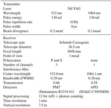
Table 1.Characteristics of Mie lidar.
Transmitter
Laser Nd:YAG
Wavelength 532 nm 1064 nm
Pulse energy 130 mJ 130 mJ
Pulse repetition rate 10 Hz
Pulse width 8 ns
Beam divergence 0.2 mrad 0.2 mrad
Receiver
Telescope type Schmidt-Cassegrain
Telescope diameter 30.5 cm
Focal length 3048 mm
Field of view 1 mrad
Polarization P and S none
Number of channels 3 1
Interference filter
Center wavelength 532.0 nm 1064.1 nm
Bandwidth (FWHM) 0.29 nm 0.38 nm
Transmission 0.66 0.58
Detectors PMT APD
(Hamamatsu R3234-01) (EG&G C30956EH) Signal processing 12 bit A/D+photon counting
Time resolution 1 min Vertical resolution 7.5 m
2 Characteristics of the lidar system and observed parameters
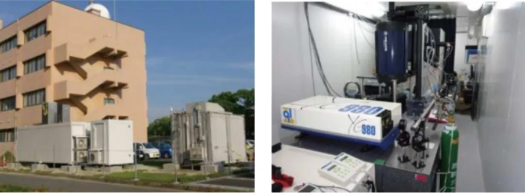
Mie lidar and ozone DIAL were installed in a container with dimensions of about 228 cm (width) by 683 cm (length) by 255 cm (height), as shown in Fig. 1. Mie lidar is a two-wavelength (532 and 1064 nm) polarization lidar based on a neodymium-doped yttrium–aluminum–garnet (Nd:YAG) laser; the characteristics are summarized in Table 1. The out-put energy at 532 and 1064 nm was 130 mJ, with a pulse repetition rate of 10 Hz. The diameter of the receiving tele-scope was 30.5 cm. The output signals from the photomulti-plier tubes (PMT) and a silicon avalanche photodiode (APD) were processed by transient recorders with a 12 bit analog to digital converter and a photon counter.
The data analysis methods of Mie lidar and ozone DIAL have been described by Uchino et al. (2012b) and Uchino et al. (2014), respectively. We summarize the observation pa-rameters obtained by Mie lidar. The backscattering ratioRis defined as
R=(BR+BA)/BR, (1)
Ander-Figure 1.The Mie lidar and ozone DIAL (right picture) were installed in the container at the left on the ground (left picture).
son et al. (2003), and Cattrall et al. (2005). The following is a summary of their lidar ratios at 532 nm:
– Asian dust 47±18 sr (Sakai et al., 2003);
– dust (spheroids) 42±4 sr, southeastern Asia pollution 58±10 sr (Cattral et al., 2005);
– Aerosol Characterization Experiment (ACE) -Asia pol-lution (fine-dominated, submicron portion) 50±5 sr, dust (coarse-dominated, dust-like chemistry, super-micron portion) 46±8 sr (Anderson et al., 2003). As a simplification, we used the same value for both Asian dust and pollutant aerosols. To calculate BR, we used the at-mospheric molecular density profiles obtained by operational radiosondes at the Fukuoka District Meteorological Obser-vatory (33.58◦N, 130.38◦E), Japan Meteorological Agency
(JMA). The aerosol extinction coefficient was calculated by multiplying BA by LR.
The total volume depolarization ratioDwas defined as D=S/(P+S)×100(%), (2) where P and S are the parallel and perpendicular compo-nents of the backscattered signals, respectively. The particle depolarization ratioDpwas obtained from the equation
Dp=(D×R−Dm)/(R−1), (3) where Dm is the atmospheric molecular depolarization
ra-tio. We used aDmvalue of 0.37 % for this lidar system; we
calculatedDmfrom the spectral transmission data of the
in-terference filter at 532 nm and the Rayleigh backscattering cross sections (Sakai et al., 2003). The value ofDpindicates
whether the particles are spherical or non-spherical; large values indicate the presence of non-spherical particles. The backscatter-related Ångström exponent, Alp, the qualitative indicator of aerosol particle size, is defined by
BA(λ)∝λ−Alp, (4)
whereλis the wavelength. Larger values of Alp indicate the predominance of smaller (i.e., submicrometer-sized) parti-cles. The vertical resolution of these observational parame-ters was 150 m, and the time resolution was set to be 1 h for comparison with the Model of Aerosol Species in the Global Atmosphere (MASINGAR)-mk2 (Yukimoto et al., 2012). The lowest altitude of Mie lidar measurement was 225 m due to the imperfect overlap of the transmitter–receiver optical axes of the lidar system.
The ozone DIAL consisted of a Nd:YAG laser and a 2 m long Raman cell filled with CO2 gas that generated four
Stokes lines from stimulated Raman scattering by CO2; the
characteristics are summarized in Table 2. In this study, we used three Stokes lines (276, 287, and 299 nm). The output energies of these Stokes lines were about 8–9 mJ per pulse, with a pulse repetition rate of 10 Hz. The receiving telescope diameters were 10 cm for boundary layer ozone measure-ments and 49 cm for free-tropospheric-ozone measuremeasure-ments. The Mie lidar and ozone DIAL were synchronized by two pulse-delay generators.
The 276/287 nm and 287/299 nm wavelength pairs were used for ozone DIAL measurements in the altitude ranges 0.57–2.0 and 2.0–6.0 km, respectively. The effective vertical resolutions were 270 m for 0.57–2.0 km and 540 m for 2.0– 6.0 km, respectively (Uchino et al., 2014). The time resolu-tion was set to 1 h to facilitate comparison with MRI-CCM2. An aerosol correction was not made for ozone retrieval. Next, we report the continuous lidar observational results made at Saga from 20 March to 31 March 2015.
3 Ozone DIAL data
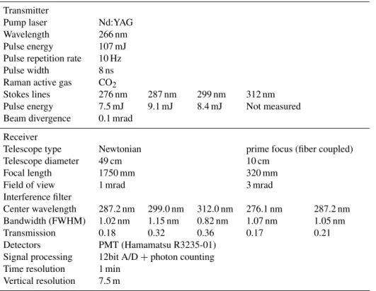
ar-Table 2.Characteristics of the tropospheric ozone DIAL system.
Transmitter
Pump laser Nd:YAG Wavelength 266 nm Pulse energy 107 mJ Pulse repetition rate 10 Hz Pulse width 8 ns Raman active gas CO2
Stokes lines 276 nm 287 nm 299 nm 312 nm Pulse energy 7.5 mJ 9.1 mJ 8.4 mJ Not measured Beam divergence 0.1 mrad
Receiver
Telescope type Newtonian prime focus (fiber coupled)
Telescope diameter 49 cm 10 cm
Focal length 1750 mm 320 mm
Field of view 1 mrad 3 mrad
Interference filter
Center wavelength 287.2 nm 299.0 nm 312.0 nm 276.1 nm 287.2 nm Bandwidth (FWHM) 1.02 nm 1.15 nm 0.82 nm 1.07 nm 1.05 nm
Transmission 0.18 0.32 0.36 0.17 0.21
Detectors PMT (Hamamatsu R3235-01) Signal processing 12bit A/D+photon counting
Time resolution 1 min Vertical resolution 7.5 m
eas where there were no observational data or the errors were larger than 10 %. The errors were computed from the lidar signal-to-noise ratios by use of Poisson statistics. Regions surrounded by a black rectangle are areas where the data were affected by aerosols and/or clouds withR larger than 2 at 299 nm. We calculatedR assuming LR=50 sr, without correcting for attenuation by ozone absorption. In the lowest row of Fig. 2a, we show hourly data of surface oxidant volume mixing ratios (Ox) at Takagimachi in Saga measured
by the Saga Prefectural Environmental Research Center (https://www.pref.saga.lg.jp/web/at-contents/kankyo1/ shisetsu/_40810/_41304/_67819.html). Takagimachi is located about 2.8 km northeast of the ozone DIAL site. Because the surface Ox was observed by a UV photometer,
the contribution of other components such as peroxyacetyl nitrate (PAN) to oxidant concentrations was extremely low, and the oxidant volume mixing ratio was considered to be that of ozone.
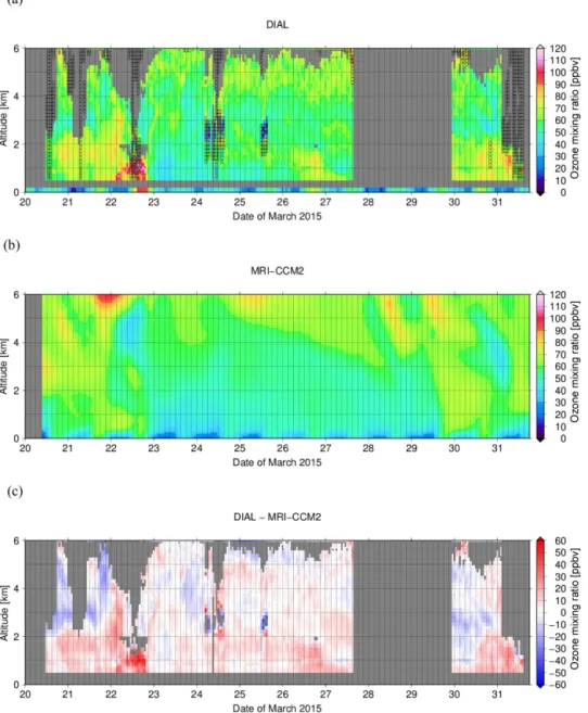
Figure 2a indicates that the ozone volume mixing ra-tios measured by DIAL were usually about 50–70 ppbv dur-ing the study period. Comparatively high ozone concentra-tions, >75 ppbv, were detected at altitudes of 0.57–3 and 0.57–2 km on 20–23 March and 30–31 March, respectively. Notably high ozone volume mixing ratios of 90–110 ppbv at altitudes of 0.57–1.5 km were observed from 03:00 to 20:00 JST on 22 March. These high ozone concentrations were also seen in the surface-photochemical-oxidants data, i.e., the Ox equaled 92–101 ppbv from 15:00 to 21:00 JST
on 22 March, as shown in the lowest row in Fig. 2a. The
maximum concentration of Ox was 101 ppbv at 16:00 JST.
This maximum value was far above the environmental qual-ity standard of 60 ppbv for hourly photochemical oxidants in Japan (https://www.env.go.jp/en/air/aq/aq.html).
3.1 Comparison of DIAL data with MRI CCM-2
MRI-CCM2 is a global model that simulates chemical and physical processes that affect the distribution and evolution of ozone and other trace gases from the surface to the strato-sphere (Deushi and Shibata, 2011). Uchino et al. (2014) have provided an outline of MRI-CCM2. The vertical res-olution of the model increases from about 100 to 600 m from the surface to 6 km. The time step of the transport (chemistry) scheme is 30 (15) min. We used hourly model output data. The horizontal resolution is about 110 km. We examined whether or not the model could simulate DIAL observational results. MRI-CCM2 simulated the DIAL ob-servations reasonably well. However, MRI-CCM2 predicted high ozone concentrations of 50–60 ppbv and could not re-produce the concentrations of 90–110 ppbv observed with DIAL below an altitude of 1.5 km during 03:00–20:00 JST on 22 March 2015.
Figure 2.Time–altitude cross sections of(a)ozone volume mixing ratios observed by DIAL over Saga from 11:10 JST on 20 March to 14:33 JST on 31 March 2015,(b)the ratios simulated by a modified MRI-CCM2 for 20–31 March 2015, and(c)the difference between the observed and simulated ozone volume mixing ratios(a–b). Gray regions indicate areas where there were no observational data or the statistical errors were larger than 10 %. Regions enclosed with black rectangles are areas where the data were affected by aerosols and/or clouds. The lowest row in(a)shows photochemical oxidant (ozone) volume mixing ratios at Takagimachi in Saga as measured by the Saga Prefectural Environmental Research Center.
fields toward the reanalysis data. In addition, we changed the emission inventory of Regional Emission inventory in Asia version 1.1 (REAS 1.1) (Ohara et al., 2007) to the REAS 2.1 emission inventory in 2007 (Kurokawa et al., 2013) and the NO2/NOx emissions ratio from 5 to 15 % by volume,
which is within the range of uncertainty (Carslaw, 2005). The emission inventory of NOxincreased about 50 % from REAS
1.1 to REAS 2.1. Figure 2c shows the differences between the observed and simulated ozone-mixing ratios. Simulated ozone volume mixing ratios were about 60–70 ppbv below an
altitude of 1.5 km from 14:00 JST on 21 March to 21:00 JST on 22 March 2015, lower by about 20–50 ppbv compared with the DIAL results. Moreover, MRI-CCM2 predicted high ozone concentrations half a day earlier than the DIAL obser-vations.
Figure 3.Time–altitude cross sections of(a)backscattering ratios,(b)total volume depolarization ratios, and(c)particle depolarization ratios forR≥2.0 at 532 nm observed by Mie lidar at Saga from 09:24 JST on 20 March to 14:34 JST on 31 March 2015. Lidar observations
were not available from 15:56 JST on 27 March to 21:58 JST on 29 March 2015 mainly because of rainy or cloudy conditions. Gray regions are areas where there were no observational data or where the observations were affected by clouds.
by Mie lidar and assuming LR=50 sr in the wavelength range 276–299 nm based on Eqs. (6) and (7) in Uchino and Tabata (1991). These biases were not large because the 276/287 nm and 287/299 nm wavelength pairs are suitable for measurements of ozone in the boundary layer and the free troposphere, respectively (Nakazato et al., 2007). As mentioned earlier, ozone DIAL data with a statistical error smaller than 10 % were used in this study. Therefore, the un-certainty in the ozone DIAL data was estimated to be smaller than 22 %, and the mean value of the uncertainty was 12 %. A model with higher horizontal resolution might be necessary
to more realistically simulate high surface ozone concentra-tion events in the planetary boundary layer.
4 Mie lidar data
Figure 3a, b, and c show time–altitude cross sections of the backscattering ratio (R), the total volume depolarization ra-tio (D), and the particle depolarizara-tion rara-tio (Dp),
Figure 4.Hourly (JST) data of surface PM2.5(red line) and Ox(blue line) measured by the Saga Prefectural Environmental Research Center for 20–31 March 2015. The volume mixing ratio of Oxwas considered to be that of ozone.
on 29 March 2015, mainly because conditions were rainy or cloudy. We made quality checks of Mie lidar data. Gray re-gions are areas where there were no observational data or the data were affected by clouds.
Aerosol layers withRin the range 2–4 almost always ex-isted below an altitude of 2.5 km during 20–31 March 2015. An event of high aerosol loading with large values of R (>8) was observed below altitudes of 1.5 km during 03:00– 21:00 JST on 22 March, when the values of D were small (the mean±standard deviation was 3.9±2.1 %) compared with those before and after the event. The values of D were larger than 7.9±2.1 % from 15:00 JST on 21 March through 15:00 JST on 23 March, except for 03:00–21:00 JST on 22 March. The main aerosol component during the event might have been submicrometer-sized spherical particles, because Dp was small (4±2 %), and the wavelength ex-ponent Alp was large (1.3±0.3). In contrast, the main aerosol particles before and after the event may have been supermicrometer-sized, nonspherical mineral dust particles becauseDpwas comparatively large (13±3 %) and Alp was 1.0±0.2 (Sakai et al., 2003; Cattrall et al., 2005). When there were no clouds above, R at 1064 nm was estimated assuming Alp=1.5 at the reference altitude, where very small amounts of aerosols were expected to be present, i.e., R=1.06±0.06 (D=1.2±0.5) at 532 nm in the altitude range 3–6 km. If the value of Alp was changed from 1.0 to 2.0 at the reference altitude, the uncertainty in Alp was esti-mated to be±0.2. Alp was 0.3–2.0 in the 11-day Mie lidar record. The maximum errors ofDandDpwere 0.1 and 2 %
forR >2 at 532 nm.
During the same time period, high aerosol concentrations were also observed at the surface (Fig. 4). Hourly values of the mass concentrations of particulate matter with a diam-eter of 2.5 µm or less (PM2.5)at Takagimachi measured by the Saga Prefectural Environmental Research Center were 23 µg m−3 at 10:00 JST and increased up to a maximum
value of 110 µg m−3at 15:00 JST on 22 March; the
concen-trations were greater than 82 µg m−3during 13:00–16:00 JST
and decreased to 17 µg m−3at 01:00 JST on 23 March. The
daily mean value of PM2.5 was 50.6 µg m−3 for 24 h on
22 March at Takagimachi, larger than the environmental quality standard of 35 µg m−3in Japan (https://www.env.go.
jp/en/air/aq/aq.html).
4.1 Comparison of Mie lidar data with MASINGAR mk-2
The MASINGAR-mk2 is an improved version of the MASINGAR aerosol model (Tanaka et al., 2003); it treats five aerosol species: sulfate, black and organic carbon, sea salt, and soil dust. We used emission data for sulfur dioxide and for black and organic carbon from MACCity (Granier et al., 2011). Soil dust and sea salt were represented by 10 bins with particle diameters of 0.2–20 µm. The model was coupled online with the atmospheric general circulation model MRI-AGCM3 (Yukimoto et al., 2012). The meteoro-logical fields were taken from JMA Global ANALysis data (GANAL). The horizontal resolution of the MASINGAR-mk2 was about 60 km, and the number of vertical layers was 40 from the surface to 0.1 hPa. The vertical resolutions in-creased from 100 to 600 m from the lowest level to 6 km. The time step of the transport (chemistry) scheme was 450 s, and we used hourly model output data.
Figure 5.Time–altitude cross sections of(a)aerosol extinction coefficients observed by Mie lidar at 532 nm over Saga from 09:24 JST on 20 March to 14:34 JST on 31 March 2015,(b)the coefficients simulated by MASINGAR-mk2 at 550 nm for 20–31 March 2015, and(c)the difference between the Mie lidar observations and the simulation(a–b). Gray regions represent areas where there were no observational data.
4.2 Comparison of aerosol optical depths
Figure 6 shows temporal variations in the aerosol optical depths (AODs) measured by Mie lidar at 532 nm and sky radiometer at 500 nm (Kobayashi et al., 2006; Uchino et al., 2012a) and simulated at 550 nm by MASINGAR-mk2 from 20 to 31 March. To estimate AODs from the lidar data, the extinction coefficient at 225 m was extrapolated to the ground, the extinction coefficient from 15 to 35 km was ob-served at night on the same day, and S was assumed to be 50 sr for all altitudes. When clouds and thick aerosols were present, AODs were not obtained. The sky radiometer was positioned on the roof of the building, which is four
Figure 6.Temporal variation of the aerosol optical depth (AOD) measured by Mie lidar at 532 nm (red squares) and by sky radiometer at 500 nm (blue circles), and simulated at 550 nm by MASINGAR-mk2 (green diamonds).
reference altitudes to 8.2 and 2.8 km at 12:00 and 13:00 JST on 22 March, respectively, for the lidar because the backscat-tered signals were strongly attenuated by the dense aerosol layers below 2 km. This might have caused errors in the AODs for the Mie lidar data. The possibility that the views obtained by the sky radiometer and Mie lidar differed might also account for the difference.
The model underestimated the AODs by factors of about 3.6–4 compared to the sky radiometer and lidar observa-tions. One plausible reason for that is that the model reso-lution (about 60 km) was insufficient to reproduce the ob-served prominent peak in which the obob-served AOD increased from 1.0 to 2.0 in 6 h. The other plausible reason for the underestimation is the uncertainty of the emissions inven-tories of aerosol precursors. Grainer et al. (2011) collected various emission inventories and compared them on a global scale. They found that differences in Chinese sulfur diox-ide (SO2)emissions in 2000 reached 66 % between the low-est and highlow-est emissions and concluded that there was no consensus among the different inventories for the emissions of Chinese SO2. This large variation among the inventories
indicates that there is a large error associated with the es-timate of SO2 emission in China. In their comparison, the
MACCity emission, which was used in the MASINGAR-mk2 simulation, showed the lowest amount of Chinese SO2
emission among the inventories. This might explain the un-derestimation of pollutant aerosol (sulfate) concentrations. In the MASINGAR-mk2 simulation, the dust-emission flux was estimated by a parameterized dust emission scheme and was strongly dependent on various parameters (e.g., soil tex-ture, soil wetness, land use, snow cover fraction, vegetation cover, and surface wind speed). The dust model intercompar-ison project (DMIP; Uno et al., 2006) reported that simulated amounts of dust emissions over East Asia differed sometimes by a factor of 10 among eight dust models (including the previous version of MASINGAR). These facts indicate that estimates of dust emissions are associated with large errors. To solve this problem, for example, it might be better to use the near-real-time-satellite data of SO2and nitrogen dioxide
Figure 7.Time (JST)–altitude cross sections of(a)total aerosol ex-tinction coefficients at 550 nm (color shading) and(b)ratios of dust extinction coefficient to total aerosol extinction coefficient (color shading) simulated by the MASINGAR-mk2 with potential tem-peratures (white(a) and black (b) contours) over Saga for 20– 31 March 2015. The gray regions in(b)indicate that the simulated total aerosol extinction coefficient was less than 0.02.
(NO2)provided by the Ozone Monitoring Instrument (OMI) onboard NASA’s Aura satellite (Krotkov et al., 2016), and/or to use a data assimilation technique that integrates model simulation and observational data (Yumimoto et al., 2016).
5 Discussion: origin and transport pathways of ozone and aerosol plumes
Figure 8. (a)The 72 h HYSPLIT-model backward trajectory (red line) and terrain height (black line) from Saga at 1500 m above ground level (a.g.l.) ending at 06:00 JST on 22 May 2015.(b)Time– altitude cross section of dust extinction coefficient simulated by the MASINGAR mk-2 along the trajectory path.
dust extinction coefficients to total aerosol extinction coef-ficients simulated by MASINGAR-mk2 with potential tem-peratures over Saga for 20–31 March 2015. For the event on 22 March, the model predicted dust particles (about 60– 100 %) in the altitude range 1–3 km, and it predicted sulfate (about 40–60 %) and dust (about 30–40 %) particles below 1 km. The numbers in parentheses indicate the ratio of each component’s extinction coefficient to the total extinction co-efficient. The dust particles descended to the surface in the afternoon (Fig. 7b). For the event on 30 March, MASINGAR mk-2 predicted dust particles (about 50–100 %) at altitudes of 1–6 km, and it predicted sulfate (about 50–80 %) and dust (about 0–20 %) particles below 1 km in the morning. Mie
Figure 9.Same as Fig. 8, but for 500 m a.g.l.
lidar data supported the model prediction becauseDp was
high (17±6 %) at altitudes of 1–3 km and low (10±3 %) below 1 km. For both events, small amounts of organic car-bon, black carcar-bon, and sea salt particles were predicted.
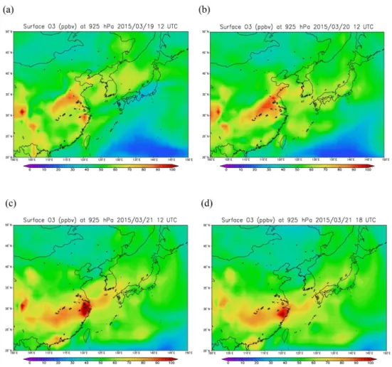
Figure 10.Horizontal maps of ozone volume mixing ratios in ppbv predicted by MRI-CCM2 for the 925 hPa pressure level (an altitude of about 760 m) at 21:00 JST (JST=UT+9) on(a)19,(b)20 and(c)21 March and(d)at 03:00 JST on 22 March 2015.
Figure 11.Time–altitude cross section of range-corrected backscatter signal at 1064 nm (color shading) and the heights of the mixed layers estimated by Mie lidar (black circles), radiosonde (white triangles), and JMA Meso-Scale Meteorological Analysis (white squares) data over Saga from 09:24 JST on 20 March to 14:34 JST on 31 March 2015.
and sulfate particles on 22 March could have been trans-ported within about 2 days from the Gobi Desert and the North China Plain (NCP), respectively, to the measurement site. The MASINGAR mk-2 simulation suggested that the dust particles emitted during 18:00–24:00 UTC on 19 March around 40◦N and 105◦E were responsible for the dust storm
captured by the Mie lidar observation. The highest concen-trations of SO2 and NO2 in the world were observed in
the NCP to the Yellow Sea and then to Saga within about 2 days.
Because it was difficult to obtain observational data of surface ozone and sulfate particles over the NCP, including Beijing, on 19–20 March, we referred to the following pa-pers with respect to those data. According to the ozonesonde measurements made by Wang et al. (2012), ozone concentra-tions ≥90 ppbv were observed over Beijing, China, in late March. Ma et al. (2016) reported a significant increase in surface ozone from 2003 to 2015 at Shangdianzi (40.65◦N,
117.10◦E), which is located about 100 km northeast of
sub-urban Beijing, and the maximum daily average 8 h con-centrations of ozone appear to have been >100 ppbv in March 2015 based on Fig. 2 in their paper. High PM2.5and
submicron aerosol concentrations have been observed in Bei-jing (Zhang et al., 2013; Sun et al., 2015). Ozone and aerosol concentrations may therefore have been high in March 2015 over the NCP.
To elucidate the vertical transport processes of the aerosol and ozone in the lower troposphere over the measurement site, we show in Fig. 11 the time variations of the heights of the mixed layers from 2 hours after sunrise to 2 hours before sunset during 09:24 JST on 20 March through 14:34 JST on 31 March 2015. These altitudes were estimated from (1) the 1064 nm range-corrected backscatter signals, with a range resolution of 15 m and a time interval of 20 min, using the wavelet covariance transform method (Baars et al., 2008; Izumi et al., 2017), and (2) signals obtained from radiosonde data at Fukuoka and the JMA mesoscale analysis (MA) data over Saga using the parcel method (Holzworth, 1964). When the mixed layers developed in the afternoon, the heights of the mixed layers (1.5–2 km) estimated by Mie lidar were sim-ilar to those estimated by MA. Although the radiosonde data at 09:00 JST on 22 March found the height of the mixed layer to be 117 m (Stull, 1988), it was difficult for Mie lidar to de-tect the mixed layer because the lowest altitude of the Mie lidar measurement was 225 m.
The dust particles that originated from the Gobi Desert ar-rived at altitudes of 1–3 km over the lidar site at 06:00 JST on 22 March. When the mixed layer developed to 1.5–2 km at 11:00–15:00 JST on 22, the dust particles were assumed to be mixed into the boundary layer and then to reach the surface by entrainment, as simulated in Fig. 7b. This may explain the sharp increase in PM2.5 concentrations at the surface after
11:00 JST, as shown in Fig. 4. A similar phenomenon was ob-served over the northern Kyushu area during the dust event in late May–early June 2014 (Uno et al., 2016). A similar high-surface-ozone event was observed by eight ozonesonde mea-surements during 6–9 June 2003 over the Seoul metropolitan region (Oh et al., 2010).
6 Concluding remarks
By using ozone DIAL and a two-wavelength polarization (Mie) lidar, we made continuous measurements of ozone and aerosol concentrations over Saga during 20–31 March 2015. High ozone and high aerosol concentrations that occurred nearly simultaneously were observed in the altitude range 0.5–1.5 km from 03:00 to 20:00 JST on 22 March 2015. The ozone volume mixing ratio was larger than 100 ppbv. The aerosol extinction coefficient and AOD at 532 nm were larger than 0.5 km−1and 1.5, respectively.
Backward trajectory analysis and the simulations by the MASINGAR mk-2 and MRI-CCM2 models indicated that mineral dust particles from the Gobi Desert and an air mass with high ozone and aerosol (mainly sulfate) concentrations that originated from the North China Plain could have been transported over the lidar site within about 2 days. Based on the lidar and surface measurement data and the simulation by the MASINGAR-mk2, there is a possibility that the air mass with high ozone and aerosol concentrations could have been transported from the lower troposphere to the surface by vertical mixing when the planetary boundary layer devel-oped in the afternoon of 22 March 2015. The combination of ozone DIAL measurements with surface in situ ozone mea-surements is very useful for studying the process of descent of high ozone concentrations in the lower troposphere to the surface and the impacts on surface air quality. Such measure-ments of pollution plumes that descend from the free tropo-sphere to the surface are highly recommended (HTAP, 2010). MRI-CCM2 could approximately reproduce the high-ozone volume mixing ratios after some modifications of physical and chemical parameters. MASINGAR mk-2 suc-cessfully predicted high-aerosol-concentration events, but the predicted peak AOD was about one-third of the observed AOD. For further improvement of these models, it will be important to continue comparing these models with ozone DIAL, Mie lidar, and surface in situ ozone and particle mea-surements.
7 Data availability
The reference and website for the data we used in the pa-per are provided in the text. The lidar and simulation data presented in the paper are available from the authors upon request ([email protected]).
Competing interests. The authors declare that they have no conflict of interest.
Akimoto, H., Mukai, H., Nishikawa, M., Murano, K., Hatakeyama, S., Liu, C., Buhr, M., Hsu, K. J., Jaffe, D. A., Zhang, L., Hon-rath, R., Merrill, J. T., and Newell, R. E.: Long-range transport of ozone in the East Asian Pacific rim region, J. Geophys. Res., 101, 1999–2010, 1996.
Ancellet, G. and Ravetta, F.: Analysis and validation of ozone vari-ability observed by lidar during the ESCOMPTE-2001 cam-paign, Atmos. Res., 74, 435–459, 2005.
Anderson, T. L., Masonis, S. J., Covert, D. S., Ahlquist, N. C., Howell, S. G., Clarke, A. D., and McNaughton, C. S.: Vari-ability of aerosol optical properties derived from in situ aircraft measurements during ACE-Asia, J. Geophys. Res., 108, 8647, doi:10.1029/2002JD003247, 2003.
Baars, H., Ansmann, A., Engelmann, R., and Althausen, D.: Con-tinuous monitoring of the boundary-layer top with lidar, At-mos. Chem. Phys., 8, 7281–7296, doi:10.5194/acp-8-7281-2008, 2008.
Bak, J., Kim, J. H., Liu, X., Chance, K., and Kim, J.: Evaluation of ozone profile and tropospheric ozone retrievals from GEMS and OMI spectra, Atmos. Meas. Tech., 6, 239–249, doi:10.5194/amt-6-239-2013, 2013.
Banta, R. M., Senff, C. J., White, A. B., Trainer, M., McNider, R. T., Valente, R. J., Mayor, S. D., Alvarez, R. J., Hardesty, R. M., Parrish, D., and Fesenfeld, F. C.: Daytime buildup and nighttime transport of urban ozone in the boundary layer during a stagna-tion episode, J. Geophys. Res., 103, 22519–22544, 1998. Carslaw, D. C.: Evidence of an increasing NO2/NOxemissions
ra-tio from road traffic emissions, Atmos. Environ., 39, 4793–4802, 2005.
Cattrall, C., Reagan, J., Thome, K., and Dubovik, O.: Variabil-ity of aerosol and spectral lidar and backscatter and extinc-tion ratios of key aerosol types derived from selected Aerosol Robotic Network locations, J. Geophys. Res., 110, D10S11, doi:10.1029/2004JD005124, 2005.
Deushi, M. and Shibata, K.: Development of a Meteorological Re-search Institute Chemistry-Climate Model version 2 for the study of tropospheric and stratospheric chemistry, Pap. Meteorol. Geo-phys., 62, 1–46, doi:10.2467/mripapers.62.1, 2011.
Draxler, R. R. and Hess, G. D.: An overview of the HYSPLIT_4 modeling system for trajectories, dispersion, and deposition, Aust. Meteor. Mag., 47, 295–308, 1998.
Eisele, H. and Trickl, T.: Improvements of the aerosol algorithm in ozone lidar data processing by use of evolutionary strategies, Appl. Optics, 44, 2638–2651, 2005.
Fernald, F. G.: Analysis of atmospheric lidar observations: some comments, Appl. Optics, 23, 652–653, 1984.
Granier, C., Bessagnet, B., Bond, T., D’Angiola, A., van der Gon, H. D.., Frost, G. J., Heil, A., Kaiser, J. W., Kinne, S., Klimont,
Hemispheric Transport of Air Pollution (HTAP) 2010, Part A: Ozone and particulate matter, edited by: Dentener, F., Keating, T., and Akimoto, H., Air Pollution Studies No. 17, United Na-tions, New York and Geneva, 278 pp., 2010.
Holzworth, G. C.: Estimates of mean maximum mixing depths in the contiguous United States, Mon. Weather Rev., 92, 235–242, 1964.
Houweling, S., Hartmann, W., Aben, I., Schrijver, H., Skidmore, J., Roelofs, G.-J., and Breon, F.-M.: Evidence of systematic errors in SCIAMACHY-observed CO2due to aerosols, Atmos. Chem. Phys., 5, 3003–3013, doi:10.5194/acp-5-3003-2005, 2005. Intergovernmental Panel on Climate Change (IPCC): Climate
Change 2013: The Physical Science Basis: Contribution of Working Group I to the Fifth Assessment Report of the Inter-governmental Panel on Climate Change, edited by: Stocker, T. F., Qin, D., Plattner, G.-K., Tignor, M., Allen, S. K., Boschung, J., Nauels, A., Xia, Y., Bex, V., and Midgley, P. M., Cambridge University Press, Cambridge, United Kingdom and New York, NY, USA, 1535 pp., doi:10.1017/CBO9781107415324, 2013. Iwasaka, Y., Yamato, M., Imasu, R., and Ono, A.: Transport of
Asian dust (KOSA) particles; importance of weak KOSA events on the geochemical cycle of soil particles, Tellus, 40B, 494–503, 1988.
Izumi, T., Uchino, O., Sakai, T., Nagai, T., and Morino, I.: Mixed layer height calculated from Mie lidar data, Tenki, submitted, 2017 (in Japanese).
Kobayashi, E., Uchiyama, A., Yamazaki, A., and Matsuse, K: Ap-plication of the maximum likelihood method to the inversion al-gorithm for analyzing aerosol optical properties from sun and sky radiance measurements, J. Meteor. Soc. Jpn., 84, 1047–1062, 2006.
Kourtidis, K., Zerefos, C., Rapsomanikis, S., Simeonov, V., Balis, D., Perros, P. E., Thompson, A. M., Witte, J., Calpini, B., Sharobiem, W. M., Papayannis, A., Mihalopoulos, N., and Drakou, R.: Regional levels of ozone in the troposphere over eastern Mediterranean, J. Geophys. Res., 107, 8140, doi:10.1029/2000JD000140, 2002.
Krotkov, N. A., McLinden, C. A., Li, C., Lamsal, L. N., Celarier, E. A., Marchenko, S. V., Swartz, W. H., Bucsela, E. J., Joiner, J., Duncan, B. N., Boersma, K. F., Veefkind, J. P., Levelt, P. F., Fioletov, V. E., Dickerson, R. R., He, H., Lu, Z., and Streets, D. G.: Aura OMI observations of regional SO2and NO2 pollu-tion changes from 2005 to 2015, Atmos. Chem. Phys., 16, 4605– 4629, doi:10.5194/acp-16-4605-2016, 2016.
Nocturnal ozone enhancement in the lower troposphere observed by lidar, Atmos. Environ., 45, 6078–6084, 2011.
Kurokawa, J., Ohara, T., Morikawa, T., Hanayama, S., Janssens-Maenhout, G., Fukui, T., Kawashima, K., and Akimoto, H.: Emissions of air pollutants and greenhouse gases over Asian re-gions during 2000–2008: Regional Emission inventory in ASia (REAS) version 2, Atmos. Chem. Phys., 13, 11019–11058, doi:10.5194/acp-13-11019-2013, 2013.
Ma, Z., Xu, J., Quan, W., Zhang, Z., Lin, W., and Xu, X.: Significant increase of surface ozone at a rural site, north of eastern China, Atmos. Chem. Phys., 16, 3969–3977, doi:10.5194/acp-16-3969-2016, 2016.
Murayama, T., Sugimoto, N., Uno, I., Kinoshita, K., Aoki, K., Hagi-wara. N., Liu, Z., Matsui, I., Sakai, T., Shibata, T., Arao, K., Sohn, B. J., Won, J. G., Yoon, S. C., Li, T., Zhou, J., Hu, H., Abo, M., Iokibe, K., Koga, R., and Iwasaka, Y.: Ground-based network observation of Asian dust events of April 1998 in east Asia, J. Geophys. Res., 106, 18345–18359, 2001.
Nakazato, M., Nagai, T., Sakai, T., and Hirose, Y.: Tropospheric ozone differential-absorption lidar using stimulated Raman scat-tering in carbon dioxide, Appl. Optics, 46, 2269–2279, 2007. Oh, I.-B., Kim, Y.-K., Hwang, M.-K., Kim, C.-H., Kim, S.,
and Song, S.-K.: Elevated ozone layers over the Seoul metropolitan region in Korea: evidence for long-range ozone transport from eastern China and its contribution to sur-face concentrations, J. Appl. Meteor. Clim., 49, 203–220, doi:10.1175/2009JAMC2213.1, 2010.
Ohara, T., Akimoto, H., Kurokawa, J., Horii, N., Yamaji, K., Yan, X., and Hayasaka, T.: An Asian emission inventory of an-thropogenic emission sources for the period 1980–2020, At-mos. Chem. Phys., 7, 4419–4444, doi:10.5194/acp-7-4419-2007, 2007.
Ohyama, H., Kawakami, S., Shiomi, K., and Miyagawa, K.: Re-trievals of total and tropospheric ozone from GOSAT thermal infrared spectral radiances, IEEE T. Geosci. Remote, 50, 1770– 1784, doi:10.1109/TGRS.2001.2170178, 2012.
Sakai, T., Nagai, T., Nakazato, M., Mano, Y., and Matsumura, T.: Ice clouds and Asian dust studied with lidar measurements of particle extinction-to-backscatter ratio, particle depolarization, and water-vapor mixing ratio over Tsukuba, Appl. Optics, 42, 7103–7116, 2003.
Stein, A. F., Draxler, R. R., Rolph, G. D., Stunder, B. J. B., Co-hen, M. D., and Ngan, F.: NOAA’s HYSPLIT atmospheric trans-port and dispersion modeling system, B. Am. Meteorol. Soc., 96, 2059–2077, 2015.
Stull, R. B.: An introduction to boundary layer meteorology, Klumer Academic Publications, 670 pp., 1988.
Sun, Y. L., Wang, Z. F., Du, W., Zhang, Q., Wang, Q. Q., Fu, P. Q., Pan, X. L., Li, J., Jayne, J., and Worsnop, D. R.: Long-term real-time measurements of aerosol particle composition in Beijing, China: seasonal variations, meteorological effects, and source analysis, Atmos. Chem. Phys., 15, 10149–10165, doi:10.5194/acp-15-10149-2015, 2015.
Tanaka, T. Y., Orito, K., Sekiyama, T. T., Shibata, K., Chiba, M., and Tanaka, H.: MASINGAR, a global tropospheric aerosol chemi-cal transport model coupled with MRI/JMA98 GCM: Model de-scription, Pap. Meteor. Geophys., 53, 119–138, 2003.
Uchino, O. and Tabata, I.: Mobile lidar for simultaneous measure-ments of ozone, aerosols, and temperature in the stratosphere, Appl. Optics, 30, 2005–2012, 1991.
Uchino, O., Kikuchi, N., Sakai, T., Morino, I., Yoshida, Y., Na-gai, T., Shimizu, A., Shibata, T., Yamazaki, A., Uchiyama, A., Kikuchi, N., Oshchepkov, S., Bril, A., and Yokota, T.: Influence of aerosols and thin cirrus clouds on the GOSAT-observed CO2: a case study over Tsukuba, Atmos. Chem. Phys., 12, 3393–3404, doi:10.5194/acp-12-3393-2012, 2012a.
Uchino, O., Sakai, T., Nagai, T., Nakamae, K., Morino, I., Arai, K., Okumura, H., Takubo, S., Kawasaki, T., Mano, Y., Matsunaga, T., and Yokota, T.: On recent (2008–2012) stratospheric aerosols observed by lidar over Japan, Atmos. Chem. Phys., 12, 11975– 11984, doi:10.5194/acp-12-11975-2012, 2012b.
Uchino, O., Sakai, T., Nagai, T., Morino, I., Maki, T., Deushi, M., Shibata, K., Kajino, M., Kawasaki, T., Akaho, T., Takubo, S., Okumura, H., Arai, K., Nakazato, M., Matsunaga, T., Yokota, T., Kawakami, S., Kita, K., and Sasano, Y.: DIAL measurement of lower tropospheric ozone over Saga (33.24◦N, 130.29◦E),
Japan, and comparison with a chemistry–climate model, At-mos. Meas. Tech., 7, 1385–1394, doi:10.5194/amt-7-1385-2014, 2014.
Uno, I., Wang, Z., Chiba, M., Chun, Y. S., Gong, S. L., Hara, Y., Jung, E., Lee, S.-S., Liu, M., Mikami, M., Music, S., Nick-ovic, S., Satake, S., Shao, Y., Song, Z., Sugimoto, N., Tanaka, T., and Westphal, D. L.: Dust model intercomparison (DMIP) study over Asia: Overview, J. Geophys. Res., 111, D12213, doi:10.1029/2005JD006575, 2006.
Uno, I., Pan, X., Itahashi, S., Yumimoto, K., Hara, Y., Kuribayashi, M., Yamamoto, S., Shimohara, T., Tamura, K., Ogata, Y., Osada, K., Kamikuchi, Y., Yamada, S., and Kobayashi, H.: Overview of long-range yellow sand and high concentration of air pollution observed over the northern Kyusyu area in late May-early June 2014, J. Jpn. Soc. Atmos. Environ., 51, 44–57, 2016.
Veefkind, J. P., Aben, I., McMullan, K., Förster, H., de Vries, J., Otter, G., Claas, J., Eskes, H. J., de Haan, J. F., Kleipool, Q., van Weele, M., Hasekamp, O., Hoogeveen, R., Landgraf, J., Snel, R., Tol, P., Ingmann, P., Voors, R., Kruizinga, B., Vink, R., Visser, H., and Levelt, P. F.: TROPOMI on the ESA Sentinel-5 Precur-sor: A GMES mission for global observations of the atmospheric composition for climate, air quality and ozone layer applications, Remote Sens. Environ., 120, 70–83, 2012.
Wang, Y., Konopka, P., Liu, Y., Chen, H., Müller, R., Plöger, F., Riese, M., Cai, Z., and Lü, D.: Tropospheric ozone trend over Beijing from 2002–2010: ozonesonde measurements and modeling analysis, Atmos. Chem. Phys., 12, 8389–8399, doi:10.5194/acp-12-8389-2012, 2012.
Yamaji, K., T. Ohara, T., Uno, I., Tanimoto, H., Kurokawa, J., and Akimoto, H.: Analysis of the seasonal variation of ozone in the boundary layer in East Asia using the Community Multi-scale Air Quality model: What controls surface ozone levels over Japan?, Atmos. Environ., 40, 1856–1868, 2006.
Yue, X. and Unger, N.: Ozone vegetation damage effects on gross primary productivity in the United States, Atmos. Chem. Phys., 14, 9137–9153, doi:10.5194/acp-14-9137-2014, 2014.