Performance of a low-cost methane sensor for ambient concentration measurements in preliminary studies

(1)

AMTD

5, 2567–2590, 2012

Performance of a low-cost methane

sensor

W. Eugster and G. W. Kling

Title Page

Abstract Introduction

Conclusions References

Tables Figures

◭ ◮

Back Close

Full Screen / Esc

Printer-friendly Version Interactive Discussion

Discussion

P

a

per

|

Dis

cussion

P

a

per

|

Discussion

P

a

per

|

Discussio

n

P

a

per

|

Atmos. Meas. Tech. Discuss., 5, 2567–2590, 2012 www.atmos-meas-tech-discuss.net/5/2567/2012/ doi:10.5194/amtd-5-2567-2012

Atmospheric Measurement Techniques Discussions

This discussion paper is/has been under review for the journal Atmospheric Measurement Techniques (AMT). Please refer to the corresponding final paper in AMT if available.

Performance of a low-cost methane

sensor for ambient concentration

measurements in preliminary studies

W. Eugster1and G. W. Kling2

1

ETH Zurich, Institute of Agricultural Sciences, Universit ¨atsstrasse 2, 8092 Zurich, Switzerland

2

University of Michigan, Department of Ecology & Evolutionary Biology, Ann Arbor, MI 48109-1048, USA

Received: 29 February 2012 – Accepted: 16 March 2012 – Published: 30 March 2012 Correspondence to: W. Eugster (eugsterw@ethz.ch)

(2)

AMTD

5, 2567–2590, 2012

sensor

Title Page

Tables Figures

◭ ◮

Back Close

Full Screen / Esc

Discussion

P

a

per

|

Dis

cussion

P

a

per

|

Discussion

P

a

per

|

Discussio

n

P

a

per

|

Abstract

Methane is the second most important greenhouse gas after CO2 and contributes to global warming. Its sources are not uniformly distributed across terrestrial and aquatic ecosystems, and most of the methane flux is expected to stem from hotspots which often occupy a very small fraction of the total landscape area. Continuous time-series

5

measurements of CH4concentrations can help identify and locate these methane hot-spots. Newer, low-cost trace gas sensors such as the Figaro TGS 2600 can detect CH4 even at ambient concentrations. Hence, in this paper we tested this sensor un-der real-world conditions over Toolik Lake, Alaska, to determine its suitability for pre-liminary studies before placing more expensive and service-intensive equipment at

10

a given locality. A reasonably good agreement with parallel measurements made us-ing a Los Gatos Research FMA 100 methane analyzer was found after removal of the strong cross-sensitivities for temperature and relative humidity. Correcting for this cross-sensitivity increased the absolute accuracy required for in-depth studies, and the reproducibility between two TGS 2600 sensors run in parallel is very good. We

con-15

clude that the relative CH4concentrations derived from such sensors are sufficient for preliminary investigations in the search of potential methane hot-spots.

1 Introduction

Methane is the second most important greenhouse gas after CO₂and increases in its concentration contributes to global warming. Its sources are not uniformly distributed

20

across terrestrial and aquatic ecosystems, and often the highest methane fluxes come from localized hotspots which may occupy only a very small area of the total land-scapes.

In the Arctic, such hotspots are generally associated with wetlands or shallow waters where sedge species with aerenchyma vent methane produced in the anoxic

sedi-25

(3)

AMTD

5, 2567–2590, 2012

sensor

Title Page

Tables Figures

◭ ◮

Back Close

Full Screen / Esc

Discussion

P

a

per

|

Dis

cussion

P

a

per

|

Discussion

P

a

per

|

Discussio

n

P

a

per

|

emissions under certain circumstances during turnover or mixing events (Eugster et al., 2003). Often, large methane fluxes from lakes are associated with ebullition (DelSon-tro et al., 2010; Eugster et al., 2011); in the Arctic this is easily visible during the cold season thanks to bubbles trapped in the ice (Walter et al., 2006). One approach to find hotspots is to move a gas analyzer across the landscape and observe the concentration

5

changes in the near-surface atmosphere that can be associated with a point-source of methane emissions. So far, this was mostly done with sensors carried by helicopter (e.g., Karapuzikov et al., 1999; Zirnig et al., 2004; Dzikowski et al., 2009; Haifang et al., 2011), by small aircraft (e.g., Hiller et al., 2011), by ground based laser scanning (e.g., Gibson et al., 2006) or surface surveying with a field-portable flame-ionization detector

10

(e.g., Schroth et al., 2012). All these approaches however fail if such hotspots are not constantly emitting methane. In such cases, a random walk survey may leave a mis-leading picture if the temporal dynamics of the methane emissions are unknown.

This is specifically the case in arctic lakes, where methane is expected to be pro-duced in the anoxic lake bottom sediments. Due to thermal stratification of the waters

15

(warmer waters on top of cold bottom waters), even high methane production at the bottom may not automatically lead to high emissions at the lake surface due to lack of mixing in the lake. Hence, a systematic sampling over longer time periods is essential to quantitatively measure the potentially short periods of high methane emissions during specific mixing or turnover events (e.g., as caused by cold-front passages; MacIntyre

20

et al., 2009). Similarly, it has been shown for soil N2O fluxes that careful consideration of spatial autocorrelation is necessary to obtain a representative flux estimate from a given area (Folorunso and Rolston, 1984).

Such systematic sampling measurements are still rather costly, and hence we carried out a field experiment with a low-cost solid state sensor that recently appeared on the

25

(4)

AMTD

5, 2567–2590, 2012

sensor

Title Page

Tables Figures

◭ ◮

Back Close

Full Screen / Esc

Discussion

P

a

per

|

Dis

cussion

P

a

per

|

Discussion

P

a

per

|

Discussio

n

P

a

per

|

level in the Arctic moist acidic tussock tundra (with a roughness length of 5.6±0.9 cm; see Eugster et al., 2005) suggests that such a sensor should show a response to hot spots within ca. 1300 m upwind under neutral atmospheric stratification. Hence, it is envisaged that with an appropriate sampling design such low-cost sensors could be placed in a regular grid with≈1 km spacing to identify times, duration, and approximate

5

locality of hot spots at the landscape scale.

2 Material and methods

2.1 The TGS 2600 gas sensor

The Taguchi Gas Sensor (TGS) 2600 (Figaro Engineering Inc., Osaka, Japan) is a low-power consumption high-sensitivity gas sensor for the detection of air contaminants

10

such as those typical for cigarette smoke (Figaro, 2005a). The general field of appli-cation of TGS sensors is leak detectors of toxic and explosive gases (Figaro, 2005b). In the case of methane, the risk of explosion starts at concentrations around 4.4 %, which is orders of magnitudes higher than ambient concentrations around 1.8 ppm (Forster et al., 2007), and hence such solid-state sensors were not sensitive enough

15

for measurements in ambient air. For example, Wong et al. (1996) reported on earlier TGS sensors that showed almost negligible change in response to non-polar gases such as hydrogen and methane. A few years later, Brudzewski (1998) reported that an older TGS 813 reacted to pulses of air and methane ranging between 1600 ppm and 4000 ppm, but not at ambient concentrations (≈1.8 ppm). Also the NGM 2611 methane

20

sensor used by T ümer and G ünd üz (2010) only is sensitive to CH4in the range 1000– 10 000 ppm. To the best of our knowledge, the TGS 2600 is the first sensor for which the manufacturer indicates a sensitivity to methane even in the ppm range (Fig. 1a). Besides methane, a sensitivity to carbon monoxide, iso-butane, ethanol and hydrogen is reported by the manufacturer (Figaro, 2005a). In addition, Kotarski et al. (2011)

re-25

(5)

AMTD

5, 2567–2590, 2012

sensor

Title Page

Tables Figures

◭ ◮

Back Close

Full Screen / Esc

Discussion

P

a

per

|

Dis

cussion

P

a

per

|

Discussion

P

a

per

|

Discussio

n

P

a

per

|

et al. (2009a) reported that their tests with the TGS 2600 were in good agreement with the manufacturer’s datasheet (Figaro, 2005a), and they also confirm a good time response of the sensor to prescribed variations in H2 concentrations in the air. Addi-tional laboratory tests were carried out by De Marcellis et al. (2009) and Morsi (2007, 2008), but no field deployments have been made to test the sensor’s performance and

5

suitability for preliminary studies. We use this terminology explicitly to specify that we do not expect such a low-cost multi-gas sensor to provide the basis for studies that require accurate and precise concentration information, but that we expect a potential for suitable use in preliminary studies such as described above.

2.2 Principle of operation

10

The TGS sensors are solid-state sensors of the size of a transistor containing a metal oxide as the sensing material, such as SnO₂Figaro (2005b). According to Ferri et al. (2009b), however, the metal oxide used for the TGS 2600 sensor is TiO2. This metal oxide, in the form of granular micro-crystals, is heated to a high temperature at which oxygen in the air is adsorbed to the crystal surface (Figaro, 2005b). In this configuration

15

the sensor has a certain resistanceR0in clean air, which is reduced under the presence of a gas to which the TGS sensor is sensitive. This reduced resistance Rs can be expressed by a power function (Figaro, 2005b)

Rs=A[C] −α

, (1)

whereRsis the actual sensor resistance,Ais a coefficient for the gas at concentration

20

[C], andαis the slope of the curve as shown in Fig. 1a. For the application in this study, we measuredR_s in a simple electronic circuit where the voltage drop over a precision resistorRLin series withRs was measured (Fig. 2).

From such a set-up, the sensor resistance can be determined as (Figaro, 2005a)

Rs=

V_c×R_L

Vout

−R_L, (2)

(6)

AMTD

5, 2567–2590, 2012

sensor

Title Page

Tables Figures

◭ ◮

Back Close

Full Screen / Esc

Discussion

P

a

per

|

Dis

cussion

P

a

per

|

Discussion

P

a

per

|

Discussio

n

P

a

per

|

where Vc is the supply voltage of 5.0 V DC, and Vout is the voltage measured over the precision resistor RL. Finally, the ratio between the actual sensor resistance RL and the clean-air resistance R0 is the sensor signal of interest to deduce methane concentrations (Fig. 1).

The main problem to overcome is the sensor’s sensitivity to ambient temperature

5

and relative humidity (Fig. 1b), for which only an empirical approach for correction is suggested by the manufacturer (Figaro, 2005b) which includes three steps: (1) identify the range of ambient temperature and humidity expected in the application; (2) obtain sensitivity curves for the target gas; (3) apply a correction to approximate the average curve.

10

2.3 Data acquisition and ancillary measurements

The TGS 2600 sensor signals were recorded by a Campbell Scientific CR3000 data logger, which also measured temperature and relative humidity using a Campbell Sci-entific sensor model CS215-L12. Laboratory tests were carried out with a Campbell Scientific CR510 data logger, both using a single-ended measurement that resolves

15

voltage signals with 666 µV resolution in the range±2500 mV, and using a differential voltage reading in the range±250 mV with a resolution of 33.3 µV relative to a 1150 mV reference signal. Test measurements were carried out every 5 s and stored in the inter-nal memory. In the field, measurements were carried out every 10 s from which 5-min averages were computed and stored on the data logger’s CF card.

20

2.4 CH4reference measurements

Field measurements with two TGS 2600 were made in parallel with a Los Gatos Research (Mountain View, CA, USA) Fast Methane Analyzer (FMA-100, serial num-ber 09-0057) on a moored floating platform on Toolik Lake, Alaska (68◦37′52′′N, 149◦36′10′′W, 720 m a.s.l.). The primary purpose of this analyzer was to measure

25

(7)

AMTD

5, 2567–2590, 2012

sensor

Title Page

Tables Figures

◭ ◮

Back Close

Full Screen / Esc

Discussion

P

a

per

|

Dis

cussion

P

a

per

|

Discussion

P

a

per

|

Discussio

n

P

a

per

|

2010). Air was drawn through the analyzer by a Varian 600 Tri Scroll pump and data were digitally recorded at 20 Hz, from which 5 min averages were computed for compar-ison with the TGS 2600 measurements. In addition, the analog output of the FMA-100 was also recorded on the CR3000 data logger to allow the synchronization of the digital data from the FMA-100 with the analog TGS 2600 data.

5

3 Results

The relevant measurement signal is the ratio between the sensor resistance under presence of methane and other trace gases (Rs) in relation to the sensor resistance under absence of these gases (R0). All attempts to directly use the voltage signal from the sensor as a measure for CH₄ concentration failed because in such a simple

ap-10

proach only≈1 % of the total variance was due to methane. Successful, however, was the approach to first convert all measuredVoutvoltage signals to sensor resistancesRs according to Eq. (2). We used a precision resistorRL=5 kΩ and a stabilized supply voltageVc or 5.0 V DC (Fig. 2).

Next we quantified the reference resistanceR0that would result from clean-air

mea-15

surements without CH₄. In principle, this should be feasible with artificial gas mixtures, but as can be seen in Fig. 1b there is such a strong dependence on temperature and relative humidity that it is not surprising that dry gas standards cannot be used. The manufacturer consequently definedR_s/R₀=1 for a relative humidity of 65 % and a temperature of 20◦C (Figaro, 2005a, see also Fig. 1b). This means that the sensor

20

must be considered a relative indicator for CH4concentrations, and hence we can sim-ply replaceR0 by the minimumRs that we find in our data. Hence, we set R0 to the sensor resistance at background levels of CH₄ at the given temperature and relative humidity that existed when this minimumR0was observed. This means that we obtain

Rs/R0≥1 by definition, which is similar to what the manufacturer specifies, but with an

25

(8)

AMTD

5, 2567–2590, 2012

sensor

Title Page

Tables Figures

◭ ◮

Back Close

Full Screen / Esc

Discussion

P

a

per

|

Dis

cussion

P

a

per

|

Discussion

P

a

per

|

Discussio

n

P

a

per

|

3.1 Sensitivity to relative humidity and temperature

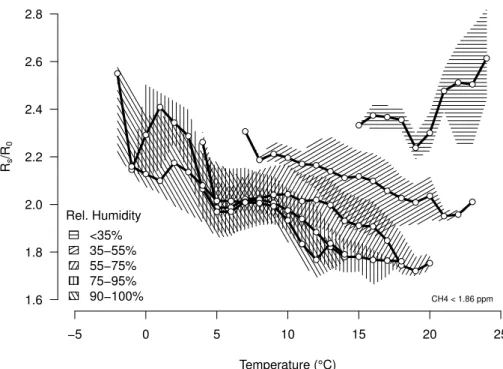
Figure 3 shows the dependence ofRs/R0on temperature and relative humidity for the whole field season 2011, which generally follows the expected pattern for relative hu-midity ranging between 35 and 100 %. At relative huhu-midity below 35 %, however, the sensor no longer obeyed the general rule that shows decreasingRs/R0 with

increas-5

ing temperatures if relative humidity was kept in a narrow range (that is, 16–35 % in our case). That the manufacturer does not mention how the sensor should behave at relative humidity below 35 % (see Fig. 1b) is an indication that the sensor does not provide reliable information at lower atmospheric moisture levels, and our experience suggests that even at 35 % relative humidity the sensor response is not as predictable

10

as the manufacturer specifies. We excluded conditions with relative humidity <40 % from further analysis.

To determine which factors actually influence the sensor signal we carried out an analysis of variance using Rs/R0 as the response variable, and methane concentra-tion, linear trend of the sensor signal over time, relative humidity and air temperature

15

as predictor variables (Table 1). This analysis indicated that over the full season 2011 more than one third (36 %) of the variance is simply attributable to the linear trend of the sensor signal, and the expected temperature and relative humidity accounted for another 34 % of the variance. This means that random variations in methane concen-trations are only responsible for 18 % of the signal variation seen in our time series.

20

Although the linear trend is most important, it is essential for practical reasons to first correct for relative humidity and temperature effects after which the corrected Rs/R0 can be translated to methane concentrations. Once the translation is complete, the lin-ear trend associated with the instrument drift (and not with the true seasonal trend) can be removed in a last step. Using this procedure would simplify the calibration

re-25

(9)

AMTD

5, 2567–2590, 2012

sensor

Title Page

Tables Figures

◭ ◮

Back Close

Full Screen / Esc

Discussion

P

a

per

|

Dis

cussion

P

a

per

|

Discussion

P

a

per

|

Discussio

n

P

a

per

|

absorption spectroscopy and use the two calibration points for removal of the temporal trend.

3.2 Removing relative humidity and temperature sensitivities

In order to estimate one single correction algorithm for the TGS 2600 sensors in gen-eral, we used the information in Fig. 1b, digitized the curves in 10◦C intervals, and then

5

fitted the following trend surface to the manufacturer’s specification:

R0

Rs

=(0.024±0.032)+(0.0072±0.0004)·rH+(0.0246±0.0007)·T_a, (3)

(n=11, adj.R2=0.9913) with rH relative humidity in percent, andTaair temperature in ◦C. To test whether this approximation can be used for our sensors we used an iterative procedure to remove the offset inR2/R0 as we defined it, and then obtained

10

best fits for the rH andTaterms for an intercept that matches the one in Eq. (3). This yielded adj.R2of 0.6337 and 0.7425 for sensors 1 and 2, respectively. The coefficients for rH were 0.0085±0.0004 and 0.0076±0.0003, and those forTawere 0.0408±0.0014 and 0.0369±0.0010 for sensors 1 and 2, respectively. This shows that there are some differences in individual sensors that must be kept in mind, but for the purpose of using

15

this sensor as a proxy for CH4concentrations in preliminary studies this is acceptable. To remove the contribution of rH andTa from ourRs/R0signals, we must recall that we used a hyperbolic approach in Eq. (3), and that the relevant information is not the absolute signal but its ratio relative to clean air at the same temperature and humidity. Hence, we remove rH andTaby computing a corrected ratio (Rs/R0)corr,

20

_R

s

R0

corr

= Rs

R0

(10)

AMTD

5, 2567–2590, 2012

sensor

Title Page

Tables Figures

◭ ◮

Back Close

Full Screen / Esc

Discussion

P

a

per

|

Dis

cussion

P

a

per

|

Discussion

P

a

per

|

Discussio

n

P

a

per

|

3.3 Conversion to CH4concentrations

As already mentioned, it is only practical to remove the linear trend in our data if we can compare methane information obtained from an in dependent sample with our sensor data; with this independent information we can convert our ratio of resistances to ppm CH4. Using a linear regression approach with our reference CH4 concentrations from

5

the FMA we obtained the following equation to convert our signal to [CH₄]_raw,

[CH4]raw=(1.8280±0.0005)+(0.0288±0.0002)·

_R

s

R0

corr

. (5)

3.4 Calibrating CH4concentrations

To simulate a typical field experiment where there is no reference gas analyzer running in parallel, we arbitrarily selected the data from the first hour of the second day (24 h

10

period) after the sensors were installed to obtain a calibration reference from the FMA at the beginning of the season. The same was done at the end of the season, using the hour starting 24 h before the end of deployment to obtain a final calibration point.

Before we applied the calibration points to remove the linear trend from our data, we investigated time lags between the TGS 2600 sensor and the FMA reference. Although

15

it is very clear that the TGS 2600 has a slower response than the FMA we could not find a consistent and relevant time lag to be considered in such a calibration approach. The real seasonal trend measured (under absence of instrument drift) by the FMA during almost 9 weeks of deployment was 0.00563 ppm week−1, whereas our sensors 1 and 2 (including the respective sensor drift) had 0.0156 and 0.0140 ppm week−1. This

20

indicates, that the trend in sensor signals increased above the real seasonal trend by 0.010 and 0.008 ppm week−1, which must be taken in account if it is not possible to obtain an initial and a terminal calibration point over a period of deployment of a TGS 2600.

Including this correction for the trend based on a calibration at the beginning

25

(11)

AMTD

5, 2567–2590, 2012

sensor

Title Page

Tables Figures

◭ ◮

Back Close

Full Screen / Esc

Discussion

P

a

per

|

Dis

cussion

P

a

per

|

Discussion

P

a

per

|

Discussio

n

P

a

per

|

period, the final corrected TGS 2600 concentration [CH₄]_corrbecomes

[CH4]corr=[CH4]raw+

1− t

∆t

· [CH4]ref,1−[CH4]raw,1

+

t

∆t

· [CH4]ref,2−[CH4]raw,2

, (6)

wheret is the elapsed time since the initial calibration time point, and ∆t is the time difference between the terminal calibration and the initial calibration in the same time units.

5

3.5 Comparison with reference instrument

After all corrections were applied, we obtained a relatively good agreement with our reference instrument for both sensors (Fig. 4). There was, however, one period start-ing around June 28–29 where both TGA 2600 sensors deviated consistently from the reference instruments for several days. Although this period may have been related to

10

smoke from wildfires (even though no smoke was observed), it was also very cold at this time with the first relevant snow fall at Toolik and in large parts of Alaska (Angeloff

et al., 2011).

In the second part of the season both TGA 2600 sensors closely followed the refer-ence concentrations, albeit with a certain reduction in peak concentrations compared

15

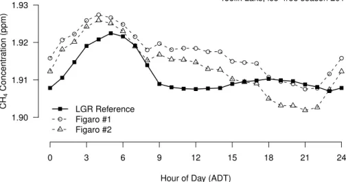
to the reference measurements: the most notable of these deviations occurred 27 and 28 July, and 3, 10, and 14 August (Fig. 4). Although the general information on the sea-sonal and diurnal patterns in CH4 can be seen in Fig. 4, the pairwise agreement of all data points from the TGA 2600 with the reference concentration is onlyR2=0.195 and 0.191, respectively, for sensors 1 and 2. This low statistical agreement can be

mislead-20

ing, because the general diurnal pattern of CH4was quite accurately resolved (Fig. 5), both in terms of change over time and absolute concentrations. The systematic devi-ations between instruments seen on some days (Fig. 4) tend to show a slightly earlier timing of the early morning peak, a less steep decrease in concentrations during the morning until 9 h ADT, and a surprising daily minimum around 21 h ADT for the TGA

25

(12)

AMTD

5, 2567–2590, 2012

sensor

Title Page

Tables Figures

◭ ◮

Back Close

Full Screen / Esc

Discussion

P

a

per

|

Dis

cussion

P

a

per

|

Discussion

P

a

per

|

Discussio

n

P

a

per

|

for more detailed studies, while showing that the sensors can still capture the essential pattern of diurnal changes in CH₄concentrations.

4 Discussion

Since smoke is associated with high levels of CO to which the TGS 2600 is sensitive according to Figaro (2005a) there is some risk of confounding effects in areas where

5

wildfire or other burning is present. However, during summer 2011, it appears that the uncertainty of the behavior of the TGS 2600 at cold temperatures (around freezing and below) led to the largest discrepancies with the reference concentration measure-ments. At least there were no reports of smoke or related odors at the site during this period. Morsi (2007) even claim that the TGS 2600 sensor is sensitive to CO2, whereas

10

the manufacturer does not mention a sensitivity for CO₂. They however do not explain why and how this sensor should respond to CO2, but if this were true, it would seriously limit the usefulness of the application of the TGS 2600 for CH4measurements. To test for this potential limitation we performed an additional ANOVA that included our CO₂ concentration measurements that were performed with a closed-path Li-7000 infrared

15

gas analyzer (Licor, Lincoln, NE, USA). Table 2 summarized the results which clearly show that CO₂ concentrations do not seriously affect the sensor’s sensitivity for CH₄; the explained variance is 18 % and perfectly matches the result in the ANOVA without CO2(Table 1). Also the relative humidity interference (21.1 % instead of 21.3 %) and the residual (unexplained) variance (11.8 % instead of 11.9 %) are only marginally affected

20

by CO2. The 3.5 % variance explained by CO2concentrations are thus simply reducing the explained variance of the temporal trend (strong reduction) and of temperature (an increase from 12.7 % to 18.0 %). Our interpretation is that this is a purely statistical artifact because (1) CO2 has its own seasonal trend which is however negative over the summer season and more in agreement with the sensor drift that we quantified

25

(13)

AMTD

5, 2567–2590, 2012

sensor

Title Page

Tables Figures

◭ ◮

Back Close

Full Screen / Esc

Discussion

P

a

per

|

Dis

cussion

P

a

per

|

Discussion

P

a

per

|

Discussio

n

P

a

per

|

with temperature; given this, the changes in explained variances in Table 2 are likely unrelated to a cross-sensitivity of the TGS 2600 as was mentioned by Morsi (2007) but not by the manufacturer (Figaro, 2005a).

Although CO2concentration by itself does not appear to be of concern for CH4 mea-surements with the TGS 2600, there is typically a tight correlation between CO₂ and

5

CO concentrations if it comes from combustion sources. Figure 1a from Figaro (2005a) indicates that the sensor’s sensitivity to CO is similar to that of CH4 for concentrations

<2–3 ppm. While this is the typical range for ambient CH₄ concentrations, the CO concentrations range between 0.03 and 0.2 ppm (Singh, 1995, p. 22), but can be up to 0.2–0.8 ppm in urban areas during summer months (Singh, 1995). At Point Barrow,

10

which can be considered the best comparison with Toolik Lake, Cavanagh et al. (1969) found about 0.09 ppm CO, which is far below the concentrations that would require a more careful consideration of CO as a confounding gas for the TGS 2600 measure-ments. In urban areas, however, a careful assessment would be needed to establish that the TGS 2600 primarily responds to CH4and not more strongly to CO.

15

Other substances that influence the TGS 2600 readings (Fig. 1a) are iso-butane, ethanol, and hydrogen. Iso-butane (R-600a) is an artificial refrigerant (C₄H₁₀) that is not expected to pose a serious problem for measurements at remote sites. Similarly, ethanol (C2H6O) is expected to have extremely low concentrations in the atmosphere because it is so highly soluble in water. Hydrogen (H2) is present at 0.6 ppm in the

av-20

erage atmosphere (Singh, 1995), but the sources are mostly anthropogenic and likely can be ignored in the remote arctic tundra.

5 Conclusions

We tested a low-cost solid state gas sensor (TGS 2600 from Figaro) for its suitabil-ity to measure ambient concentrations of CH4 in the air on the low arctic at Toolik

25

(14)

AMTD

5, 2567–2590, 2012

sensor

Title Page

Tables Figures

◭ ◮

Back Close

Full Screen / Esc

Discussion

P

a

per

|

Dis

cussion

P

a

per

|

Discussion

P

a

per

|

Discussio

n

P

a

per

|

spectrometer (FMA, Los Gatos Research). The TGS 2600 revealed a high sensitivity for relative humidity and temperature similar to that expected from the specifications by the manufacturer. After corrections for these sensitivities we obtained a realistic CH4 signal that has the quality for preliminary studies to inspect temporal patterns of CH₄ concentrations which could then inform the decision on whether a considerably more

5

expensive instrument should be deployed for high-accuracy concentration measure-ments. One realistic approach would be to install such low-cost sensors in a regular grid with≈1 km spacing to cover a landscape of interest, which would allow to identify times, duration, and approximate locality of hot spots at the landscape scale.

In the seasonal average the TGS 2600 provided realistic insight into the temporal

10

dynamics of CH₄ over Toolik Lake and also reproduced the average diurnal cycle of CH4 with an early morning concentration peak of the correct order of magnitude at approximately the correct time of day. Both the general behavior and the systematic differences from the reference instrument were similar for the TGS sensors. From this experience we suggest that the TGS 2600 can be used for preliminary assessment

15

of CH4 concentrations at sites where other gas components to which the sensor is sensitive are absent or at low concentrations, and where relative humidity is typically

>40 %. Such conditions are not only found in the low arctic, but also in rural areas of more populated zones where the distance to local CO sources can be substantial.

Acknowledgements. We acknowledge support received from the Arctic LTER grant

NSF-DEB-20

1026843 including supplemental funding from the NSF-NEON program. Gus Shaver (MBL) is acknowledged for initiating the study and supporting our activities in all aspects. We also thank Peter Pl ¨uss (ETH Zurich), Jennifer M Kostrzewski (University of Michigan) and Dustin Carroll for technical and field assistance, and Dan White (MBL) for logistical support with the boats.

References

25

(15)

AMTD

5, 2567–2590, 2012

sensor

Title Page

Tables Figures

◭ ◮

Back Close

Full Screen / Esc

Discussion

P

a

per

|

Dis

cussion

P

a

per

|

Discussion

P

a

per

|

Discussio

n

P

a

per

|

Brudzewski, K.: An attempt to apply Elman’s neural-network to the recognition of methane pulses, Sensor. Actuat. B-Chem., 47, 231–234, doi:10.1016/S0925-4005(98)00028-8, 1998. 2570

Cavanagh, L. A., Schadt, C. F., and Robinson, E.: Atmospheric hydrocarbon and carbon monox-ide measurements at Point Barrow, Alaska, Environ. Sci. Technol., 3, 251–257, 1969. 2579

5

De Marcellis, A., Di Carlo, C., Ferri, G., Stornelli, V., Depari, A., Flammini, A., and Marioli, D.: New low-voltage low-power current-mode resistive sensor interface with R/T conversion and DC excitation voltage, in: Proceedings of the 13th Italian Conference On Sensors and Mi-crosystems, 515–520, 2009. 2571

DelSontro, T., McGinnis, D. F., Sobek, S., Ostrovsky, I., and Wehrli, B.: Extreme methane

emis-10

sions from a Swiss hydropower reservoir: contribution from bubbling sediments, Environ. Sci. Technol., 44, 2419–2425, doi:10.1021/es9031369, 2010. 2569

Dzikowski, M., Klyashitsky, A., Jaeger, W., and Tulip, J.: Open path spectroscopy of methane using a battery operated vertical cavity surface-emitting laser system, Proc. SPIE, 7386, 73861H, 2009. 2569

15

Eugster, W. and Pl ¨uss, P.: A fault-tolerant eddy covariance system for measuring CH₄ fluxes, Agr. Forest Meteorol., 150, 841–851, doi:10.1016/j.agrformet.2009.12.008, 2010. 2572 Eugster, W., Kling, G., Jonas, T., McFadden, J. P., W ¨uest, A., MacIntyre, S., and Chapin III, F. S.:

CO₂exchange between air and water in an arctic Alaskan and midlatitude Swiss lake: impor-tance of convective mixing, J. Geophys. Res., 108, 4362–4380, doi:10.1029/2002JD002653,

20

2003. 2569

Eugster, W., McFadden, J. P., and Chapin III, F. S.: Differences in surface roughness, energy, and CO₂fluxes in two moist tundra vegetation types, Kuparuk Watershed, Alaska, USA, Arct. Antarct. Alp. Res., 37, 61–67, 2005. 2570

Eugster, W., DelSontro, T., and Sobek, S.: Eddy covariance flux measurements confirm extreme

25

CH₄ emissions from a Swiss hydropower reservoir and resolve their short-term variability, Biogeosciences, 8, 2815–2831, doi:10.5194/bg-8-2815-2011, 2011. 2569

Ferri, G., De Marcellis, A., Di Carlo, C., Stornelli, V., Flammini, A., Depari, A., Marioli, D., and Sisinni, E.: A CCII-based low-voltage low-power read-out circuit for DC-excited resistive gas sensors, IEEE Sens. J., 9, 2035–2041, doi:10.1109/JSEN.2009.2033197, 2009a. 2570

30

(16)

AMTD

5, 2567–2590, 2012

sensor

Title Page

Tables Figures

◭ ◮

Back Close

Full Screen / Esc

Discussion

P

a

per

|

Dis

cussion

P

a

per

|

Discussion

P

a

per

|

Discussio

n

P

a

per

|

Figaro: TGS 2600 – for the detection of air contaminants, Online product data sheet, http:// www.figarosensor.com/products/2600pdf.pdf (last access: March 2012), 2005a. 2570, 2571, 2573, 2578, 2579, 2586

Figaro: Technical information on usage of TGS sensors for toxic and explosive gas leak de-tectors, Online product information sheet, http://www.figarosensor.com/products/common%

5

281104%29.pdf (last access: March 2012), 2005b. 2570, 2571, 2572

Folorunso, O. A. and Rolston, D. E.: Spatial variability of field-measured denitrification gas fluxes, Soil Sci. Soc. Am. J., 48, 1214–1219, 1984. 2569

Forster, P., Ramaswamy, V., Artaxo, P., Berntsen, T., Betts, R., Fahey, D. W., Haywood, J., Lean, J., Lowe, D. C., Myhre, G., Nganga, J., Prinn, R., Raga, G., Schulz, M., and

Dor-10

land, R. V.: Changes in atmospheric constituents and in radiative forcing, Cambridge Univer-sity Press, 129–234, 2007. 2570

Gibson, G., van Well, B., Hodgkinson, J., Pride, R., Strzoda, R., Murray, S., Bishton, S., and Padgett, M.: Imaging of methane gas using a scanning, open-path laser system, New J. Phys., 8, 26, doi:10.1088/1367-2630/8/2/026, available at: http://www.njp.org/, 2006. 2569

15

Haifang, L., Shisheng, Z., Rui, W., and Keqiang, L.: Remote helicopter-borne laser detector for searching of methane leak of gas line, in: Prognostics and System Health Management Conference (PHM2011 Shenzhen), MU3049, 2011. 2569

Hiller, R. V., McFadden, J. P., and Kljun, N.: Interpreting CO₂fluxes over a suburban lawn: the influence of traffic emissions, Bound.-Lay. Meteorol., 138, 215–230, 2011. 2569

20

Karapuzikov, A., Ponomarev, Y., Ptashnik, I., Romanovsky, O., Kharchenko, O., and Sher-stov, I.: Helicopter lidar project for the remote methane leakage detection based on the TEA CO₂ laser radiation harmonics, in: Science and Technology, 1999, KORUS ’99, Proceedings, The Third Russian-Korean International Symposium on, vol. 2, 663–666, doi:10.1109/KORUS.1999.876253, 1999. 2569

25

Kotarski, M., Smulko, J., Czyzewski, A., and Melkonyan, S.: Fluctuation-enhanced scent sensing using a single gas sensor, Sensor. Actuat. B-Chem., 157, 85–91, doi:10.1016/j.snb.2011.03.029, 2011. 2570

MacIntyre, S., Fram, J. P., Kushner, P. J., Bettez, N. D., O’Brien, W. J., Hobbie, J. E., and Kling, G. W.: Climate-related variations in mixing dynamics in an Alaskan arctic lake, Limnol.

30

Oceanogr., 54, 2401–2417, 2009. 2569

(17)

AMTD

5, 2567–2590, 2012

sensor

Title Page

Tables Figures

◭ ◮

Back Close

Full Screen / Esc

Discussion

P

a

per

|

Dis

cussion

P

a

per

|

Discussion

P

a

per

|

Discussio

n

P

a

per

|

Society, Vol. 1–3, Conference Proceedings, 2203–2208, doi:10.1109/IECON.2007.4460098, 2007. 2571, 2578, 2579

Morsi, I.: Electronic noses for monitoring environmental pollution and building regression model, Iecon 2008: 34th Annual Conference of the IEEE Industrial Electronics Society, Vol. 1–5, Proceedings, 1668–1673, 2008. 2571

5

Reeburgh, W. S., King, J., Regli, S., Kling, G., Auerbach, N., and Walker, D.: A CH₄emission estimate for the Kuparuk River Basin, Alaska, J. Geophys. Res., 103, 29005–29013, 1998. 2568

Schmid, H. P.: Source areas for scalars and scalar fluxes, Bound.-Lay. Meteorol., 67, 293–318, 1994. 2569

10

Schroth, M. H., Eugster, W., G ´omez, K. E., Gonzalez-Gil, G., Niklaus, P. A., and Oester, P.: Above- and below-ground methane fluxes and methanotrophic activity in a landfill-cover soil, Waste Manage., doi:10.1016/j.wasman.2011.11.003, in press, 2012. 2569

Singh, H. B. (Ed.): Composition, Chemistry, and Climate of the Atmosphere, Van Nostrand Reinhold, New York, 527 pp., 1995. 2579

15

T ümer, A. E. and G ünd üz, M.: Design of a methane monitoring system based on wireless sensor networks, Sci. Res. Essays, 5, 799–805, 2010. 2570

Walter, K. M., Zimov, S. A., Chanton, J. P., Verbyla, D., and Chapin III, F. S.: Methane bubbling from Siberian thaw lakes as a positive feedback to climate warming, Nature, 443, 71–75, doi:10.1038/nature05040, 2006. 2569

20

Wong, K. K. L., Tang, Z. A., Sin, J. K. O., Chan, P. C. H., Cheung, P. W., and Hiraoka, H.: Sensing mechanism of polymer for selectivity enhancement of gas sensors, ICSE ’96 – 1996 IEEE International Conference On Semiconductor Electronics, Proceedings, 217–220, doi:10.1109/SMELEC.1996.616485, 1996. 2570

Zirnig, W., Ulbricht, M., Fix, A., and Klingenberg, H.: Helicopter-borne laser methane detection

25

(18)

AMTD

5, 2567–2590, 2012

sensor

Title Page

Tables Figures

◭ ◮

Back Close

Full Screen / Esc

Discussion

P

a

per

|

Dis

cussion

P

a

per

|

Discussion

P

a

per

|

Discussio

n

P

a

per

|

Table 1. Analysis of variance of the CH₄ sensor resistance R_s/R₀ for Toolik Lake, summer 2011.

Source of variation Df Sum Sq Mean Sq F value Pr(> F) Expl. Variance

Time trend 1 2825.29 2825.29 252 590 <2.2×10−16

*** 36.1%

Relative humidity 1 1668.82 1668.82 149 198 <2.2×10−16_*** _{21.3 %}

Methane concentration 1 1409.8 1409.8 126 041 <2.2×10−16_*** _{18.0 %}

Air temperature 1 996.4 996.4 89 081 <2.2×10−16*** 12.7 %

Residual variation 82 976 928.11 0.01 11.9 %

(19)

AMTD

5, 2567–2590, 2012

sensor

Title Page

Tables Figures

◭ ◮

Back Close

Full Screen / Esc

Discussion

P

a

per

|

Dis

cussion

P

a

per

|

Discussion

P

a

per

|

Discussio

n

P

a

per

|

Table 2.Same analysis as in Table 1, but with the inclusion of CO₂concentrations as a potential source of variation.

Source of variation Df Sum Sq Mean Sq F value Pr(> F) Expl. Variance

Time trend 1 2158.31 2158.31 193 259 <2.2×10−16_*** _{27.6 %}

Relative humidity 1 1653.44 1653.44 148 053 <2.2×10−16*** 21.1 %

Methane concentration 1 1409.8 1409.8 126 236 <2.2×10−16*** 18.0 % Air temperature 1 1407.83 1407.83 126 059 <2.2×10−16

*** 18.0 %

CO₂concentration 1 272.37 272.37 24 389 <2.2×10−16_*** _{3.5 %}

Residuals 82 975 926.66 0.01 11.8 %

(20)

AMTD

5, 2567–2590, 2012

sensor

Title Page

Tables Figures

◭ ◮

Back Close

Full Screen / Esc

Discussion

P

a

per

|

Dis

cussion

P

a

per

|

Discussion

P

a

per

|

Discussio

n

P

a

per

|

0.01 0.1 1 10

1 10 100

Rs/Ro

Gas Concentration (ppm) Air Methane

Carbon monoxide

Iso-butane Ethanol Hydrogen

0.1 1 10

-20 -10 0 10 20 30 40 50 Rs/Ro

Ambient Temperature (˚C)

R.H. 35% 65% 95%

R

s

/R

0

TGS 2600

Sensitivity Characteristics

TGS 2600

Temperature/Humidity Dependency

R

s

/R

0

(a) (b)

(21)

AMTD

5, 2567–2590, 2012

sensor

Title Page

Tables Figures

◭ ◮

Back Close

Full Screen / Esc

Discussion

P

a

per

|

Dis

cussion

P

a

per

|

Discussion

P

a

per

|

Discussio

n

P

a

per

|

R_s

R_L

Fig. 2.Sensor configuration used in this study. The variable sensor resistance Rs was

(22)

AMTD

5, 2567–2590, 2012

sensor

Title Page Abstract Introduction Conclusions References Tables Figures ◭ ◮ ◭ ◮ Back Close

Full Screen / Esc

Printer-friendly Version Interactive Discussion Discussion P a per | Dis cussion P a per | Discussion P a per | Discussio n P a per |

−5 0 5 10 15 20 25

1.6 1.8 2.0 2.2 2.4 2.6 2.8 Temperature (°C) Rs /R 0 ● ● ● _● ● ● ● ● ● ● ● ● ● ● _● ● ● ● ● ● ● ● _● ● ● ● ● ● ● ● ● ● ● ● _● ● ● ● _● ● ● ● ● ● ● ● ● ● ● ● ● ● ● ● _● ● ● ● ● ● ● _● _● ● ● ● ● ● ● ● ● ● ● ● ● _● ● ● ● ● ● Rel. Humidity <35% 35−55% 55−75% 75−95%

90−100% CH4 < 1.86 ppm

Fig. 3.Observed sensor sensitivity to ambient temperature and relative humidity at CH₄ con-centrations<1.86 ppm during the full 2011 field season at Toolik Lake. At relative humidities

≥35 % the sensor resistance ratio follows the expected curves in Fig. 1b with an offset, but

(23)

AMTD

5, 2567–2590, 2012

sensor

Title Page

Tables Figures

◭ ◮

Back Close

Full Screen / Esc

Discussion

P

a

per

|

Dis

cussion

P

a

per

|

Discussion

P

a

per

|

Discussio

n

P

a

per

|

15 Jun 22 Jun 29 Jun 06 Jul 13 Jul 20 Jul 27 Jul 03 Aug 10 Aug 17 Aug 24 Aug 1.85

1.90 1.95 2.00

CH

4

Concentr

ation (ppm)

LGR Reference Figaro #1 Figaro #2

(24)

AMTD

5, 2567–2590, 2012

sensor

Title Page

Tables Figures

◭ ◮

Back Close

Full Screen / Esc

Discussion

P

a

per

|

Dis

cussion

P

a

per

|

Discussion

P

a

per

|

Discussio

n

P

a

per

|

● ●

● _● ●

● ●

●

● ● ●

● ●

● ● ●

● ● _●

● ● ●

●

0 3 6 9 12 15 18 21 24

1.90 1.91 1.92 1.93

Hour of Day (ADT)

CH

4

Concentr

ation (ppm)

●

LGR Reference Figaro #1 Figaro #2

Toolik Lake, ice−free season 2011