A direct technique for the homogenization of periodic beam-like struc- tures by transfer matrix eigen-analysis

A direct technique for the homogenization of periodic beam-like

struc-tures by transfer matrix eigen-analysis

Abstract

To homogenize lattice beam-like structures, a direct approach based on the matrix eigen- and principal vectors of the state transfer matrix is proposed and discussed. The Timoshenko couple-stress beam is the equivalent con-tinuum medium adopted in the homogenization process. The girders unit cell transmits two kinds of bending moments: the first is generated by the couple of the axial forces acting on the section nodes, the other one is due to the moments directly applied at the node sections by the adjacent cells. This latter moment is modelled as the resultant of couple-stress. The main ad-vantage of the method consists in to operate directly on the sub-partitions of the unit cell stiffness matrix. Closed form solutions for the transmission principal vectors of the Pratt and X-braced girders are also attained and em-ployed to calculate the stiffnesses of the related equivalent beams. Unit cells having more complex geometries are analysed numerically. As a result, the principal vector problem is always reduced to the inversion of a well-condi-tioned (3 3) matrix employing the direct approach. Hence, no ill-condi-tioning problems, affecting all the known transfer methods, are present in the proposed method. Finally, comparing the predictions of the homoge-nized models with the finite element (f.e.) results of a series of girder, a val-idation of the homogenization method is performed.

Keywords

Pratt, X-braced and Warren girders – Beam like lattice – Timoshenko couple-stress beam – Homogenization.

Notations

Latin letters:

A

stiffness matrix of the inner constrained unit cell

A reduced stiffness matrix of the inner constrained unit cell

,

c d

A A

chord and diagonal cross section areas

, ,

c t d

I I I

_{chords, battens and diagonals second order central moment}

i

d

dof’s vector of the girder section

i

i

f

vector of the alternative static quantities on the section i

G

state transfer matrix

t

h l



_{girder height}

K

unit cell stiffness matrices

, ,

c d t

l l l

length of the unit cell chords, diagonal and battens

L

girder span

i

M

_{bending moment generated by the anti-symmetric axial forces on the girder section}

i

Antonio Gesualdoa

Antonio Iannuzzoa

Giovanni Pio Pucillob

Francesco Pentab _*

a _{Dipartimento di Strutture per l'Ingegneria} e l'Architettura, Università degli Studi di Napoli Federico II, Napoli, Italia. E-mail: [email protected],

[email protected]

b _{Dipartimento di Ingegneria Industriale,} Università degli Studi di Napoli Federico II, Napoli, Italia. E-mail: [email protected], [email protected]

*Corresponding Author

http://dx.doi.org/10.1590/1679-78254362 Received August 04, 2017

ˆ ,

_{i i}

m m



resultant of the nodal bending moments and difference between the top and bottom nodal bending moment on the section i

ˆ

_i

n

axial force on the girder section

i

,

l i i

p p

forces vector of the node il and of the section

i

R

radius of curvature

i

s

state vector of the section i

ˆ

_i

u

axial displacement of the section

i

,

u v axial and transversal displacements of the equivalent beam cross section

, l l i i

u v horizontal and vertical displacements of the node il

i

V

_{shear force on the girder section i}

Greek letters:

c d

 

axial stiffness parameters of chords and diagonals

b



equivalent bending stiffness

p



_{couple stress bending}

,

p a

 

_{coefficient matrix determinants}

δ δl_i, _i displacements vector of the node il and of the section

i

,

  dummy variables

c d t

  

bending stiffness parameters of chords, diagonals and battens

d



_{slope angle of the girder diagonals}

a



_{equivalent axial stiffness}

V



_{equivalent shear stiffness}



rotation of the equivalent beam cross section

l i



rotation of the node il

ˆ ,

_{i i}

 



the symmetric and anti-symmetric parts of the nodal rotations of the girder section

i

i



rotation of the section

i

Subscripts:

a, b, v axial, bending and coupled shear-bending force or displacement components

1 INTRODUCTION

The response of these types of structures to the service loads is usually analysed in a CAE environment. A f.e. discrete system models the girder-like structures and one of the solution methods for the structural framework problems is then applied to find the unknowns mechanical parameters.

If a considerable number of bays or unit cells composes the girder beam, to avoiding strong calculations charges especially during the preliminary design phase, it may be convenient to approximate its mechanical behav-iour by a continuum 1-D model, whose properties come from those of the unit cell by a suitable homogenization method. Frequently, this kind of approach also offers the additional advantage of providing analytical closed form solutions for the problem at hand. Moreover, the continuous approximation may be employed as a means of tran-sition to a coarser discrete system with a lower and more tractable set of kinematic and static unknowns.

To analyse correctly the in plane bending of periodic lattice structures, the classical continuum theory does not provide an acceptable approximation. In fact, several micropolar equivalent models have been reported for the analysis of planar lattices (Noor (1988), Bazant and Christensen (1972), Kumar and McDowell (2004), Bakhvalov and Panasenko (1989), Segerstad et al. (2009), Wang and Strong (1999), Warren and Byskov (2002), Onck (2002), Martinsson and Babuška (2007), Liu and Su (2009), Dos Reis and Ganghoffer (2012), Trovalusci et al. (2015), Bacigalupo and Gambarotta (2014), Hasanyan and Waas (2016)). While, the studies on the micro-polar models for analysing beam like lattices have not yet achieved the same advances. As far as the authors are aware, only few papers have specifically addressed this topic. In Noor and Nemeth (1980), Salehian and Inman (2010), a rational approach is presented where stiffness parameters of the effective continuum model were obtained using energy equivalence concepts. Nodal displacements of the unit cell were got in an approximated way by a Taylor expansion of the kinematical model of the substitute continuum. Then, the equivalent stiffnesses were derived by equating the potential and kinetic energies of a unit cell of the lattice beam to those of the equivalent continuum. This approach leads to two questionable stiffness couplings between the symmetric and anti-symmetric components of the shear stresses and between the bending and couple stress moments, making difficult the solution of the equilibrium equa-tions of the equivalent beam, also for the simplest loading and constraint condiequa-tions. In Romanoff and Reddy (2014) the modified couple stress Timoshenko beam theory (Ma et al. (2008, Reddy (2011) is used to analyse the trans-versal bending of web-core sandwich panels. The equivalent polar bending stiffness was determined by invoking the spring analogy criterion. According to this rule, along the substitute beam, the ratio of the couple stress moment to the total bending moment is given by the ratio of the chords bending moment to the moment of the couple of axial forces acting in the panels faces. As it is shown in Gesualdo et al (2017b), this assumption unfortunately leads to an overestimation of the polar bending stiffness.

In this paper, the state transfer matrix eigen-analysis method is applied to evaluate the properties of the mi-cropolar medium substituting a periodic beam-like structure. So far, the transfer matrix methods have been applied mostly for the dynamic analysis of repetitive or periodic structures (Mead (1970), Meirowitz and Engels (1977), Yong and Lin (1989), Langley (1996), i.e.). Just recently, it has also been used for the elasto-static analysis of pris-matic, curved and pre-twisted repetitive beam like lattices made of pin-jointed bars (Stephen and Zhang (2004, 2006, Stephen and Ghosh, 2005). The main advantage of this method consists in evaluating both the Saint-Venant decay rates and the load transmission modes by carrying out an eigen-analysis of the unit cell transmission matrix

G

. Although conceptually simple, its practical implementation is problematic, since the

G

matrix is defective and ill-conditioned. Consequently, the Jordan block structure of

G

is very difficult to be determined numerically.

The method can be easily extended also to more complex unit cell geometries composed of two or more bays. In these cases, eigen and principal vectors of

G

must be determined numerically solving a linear algebraic system for the five kinematical quantities defining the deformed shape of the cell nodal sections. However, since the cell elastic responses are invariant for rigid translations, all the unit eigen-/principal vectors are defined up to the axial and transversal displacement components uˆ and v. Hence, the eigen/principal vector problem is always reduced

to the inversion of a (3 3) matrix that is well conditioned and allows an accurate evaluation of the force transmis-sion modes.

The real capability of the resulting equivalent beams in reproducing the behaviour of real discrete beam-like lattice structures is finally assessed performing some sensitivity analyses by a set of f.e. models. As a consequence, the accuracy of the results associate to the homogenized beams in a wide range of lattice parameters variation, satisfactorily validates the suggested direct technique.

2. EIGEN-ANALYSIS OF THE TRANSFER STATE MATRIX

To depict in a clear and concise manner the homogenization method we propose, some examples of immediate technical and engineering interest are examined in this section. Specifically, the Pratt girder problem is analysed in detail while the main results related to the X-braced girder are synthetically shown. The Vierendeel girder scheme, equally significative as the previous ones, is not explicitly considered since its solution can be obtained from those of the Pratt and X-braced girder by simply neglecting the stiffnesses of the diagonal rods. Finally, the problem of the Warren girder is also considered and the peculiar features of the method, making it more convenient when unit cell eigen and principal vectors can only be determined numerically, are highlighted.

d

h

=

lt

s = lc

s = 2 lc (E I )c c

(E A )c c

(E

I )

/2

w

w

(E I )c c

(E A )c c

(E

I

)/

2

w

w

(E Id_{d )} (E Ad ₎

d

(E I )c c

(E A )c c

(E I )c c

(E A )c c

(E

I

)/

2

w

w

(E

I )

/2

w

w

(E Id ₎ d (E Ad ₎

d

(E Id_{d )} (E Ad ₎

d (E

I )dd (E A

) dd

(E

I )

/2

w

w

(E

I

)/

2

w

w

(E I )c c

(E A )c c

(E I )c c

(E A )c c

(E I )c c

(E A )c c

(E I )c c

(E A )c c

h

=

lt

s = lc

h

=

lt

a)

b)

c)

a)

b)

c)

d

d d

Figure 1: Beam-like lattices and their unit-cells: Pratt girder (a), X-braced girder (b) and Warren girder (c).

2.1 Pratt and X-braced girders

The unit cell of a Pratt girder is schematically represented in Figure 1. It is made up of two straight parallel chords rigidly connected both to the webs and to the diagonal. All the cell members are Bernoulli-Euler beams. The top and bottom chords have the same section whose area and second order central moment are denoted

A

_c and

central moment of the transverse webs is indicated with

I

w. However, to account for girder periodicity, the two

vertical beams of the unit cell will have second order moment equal to the half part of

I

w.

To identify any static or kinematical quantity related to the nodal section i of the girder, the sub-script i will be adopted, see Figure 2. To distinguish between the joints or nodes of the same section, the superscripts t or b are used, depending on whether the top or bottom chord is involved. Finally, in a coherent manner, top and bottom nodes of the section i are labelled

i

t or

i

b.

In what follows, we denote:

δt_i [ , ,u v_it _it t T_i] and δ_ib [ , ,u v_ib b_i _ib T] (1)

the displacement vectors of the joints _it _{and i}b_{, where} (.) _and (.)

i i

u v are the displacement components of the joint (.)

i

and ( .)

i

 is the rotation. Therefore, the displacement vector of the nodal section i is:

δ δtT,δbT T .

i i i

 

 _ _

 

Similarly, the nodal forces applied on the joints

i

t and

i

b of the cell are:

, , T and , , T

t t t t b b b b

i _F F mi x i y i_ i  _F F mi x i y i_

p p (2)

where (.) _and (.)

i x i y

F F are respectively the axial and transversal force components and

m

_i(.) the couple on the joint

(.)

i

. Thus, the vector of the nodal forces acting on the section i of the girder is: _i  _ t T_i , b T_i _T.

 

p p p

1 2 3 i-cell N-1 N

ib

i-1b

it

i-1t

1b

0b

1t

0t

2b

2t

Nb

N-1b

Nt

N-1t

y x

Fi x

mt i

Fi xt

Fi yt

ut i

, ,

,t i

vt i

Fi-1 yt ,vti-1

mt i-1,ti-1

Fi-1 xt ,uti-1

Fi-1 yb ,vbi-1

Fi-1 yb ,vbi-1

mb i-1,bi-1

Fi x

mb i

Fi xb

Fi yb

ub i

,

,

,b i

vb

i

O

Figure 2: Unit cell nodes numbering with girder nodal inner forces and displacements

In what follows we assume that the positive components of

p

_i are those acting according the reference axis on the right side of the cell (see Figure 2). Thus, the cell i, bounded by the sections i-1 and i respectively on the left and right sides will be loaded by the nodal force vectors



p

i1 and

p

i.

The Pratt cell stiffness matrix

K

can be computed following the standard method adopted in the f.e. analysis, that is by additively assembling the stiffnesses of the beam components through the Boolean topological matrices. For our purposes, it is however more convenient to adopt alternative static and kinematic quantities to the standard ones of Figure 2 and eq. (1) and (2). More precisely, to identify the deformed configuration of a nodal section, we

use the mean axial displacement ˆ

2

t b

i i

i

u u

u   , the section rotation

b t

i i

i t

u u

l

   being lt the web length, the

ˆ

2

t b

i i

i

 

   and .

2

t b

i i

i

 

  

The static quantities conjugates of the previous kinematic variables are: the axial force , 2

b t

i i

i

F F

n   the

bending moment



b t



i i i t

M  F F l generated by the anti-symmetric axial forces, the shear force t b

i i y i y

S F F ,

the resultant of the section bending moments

ˆ

t b

i i i

m



m



m

_{and, finally, the difference between the same moments}

t b

i i i

m





m



m

.

The standard kinematic quantities

δ

_i can be expressed as functions of the new ones d_{i  }uˆ_i _i v_i ˆ_i _i_

through the matrix equation:

δ

_i



hd

_i

,

being:

1

1 0 0 0

2

0 0 1 0 0

0 0 0 1 1

1

1 0 0 0

2

0 0 1 0 0

0 0 0 1 1

t

t

l

l

 

 _ 

 

 

 

 

 

 



 

 

 

 

 

 _ 

 

 

h _.

Denoting by f_{i  }_nˆ_i M_i S_i mˆ_i m_i_ the vector of the alternative static quantities given by f_i h pT _i, the unit cell stiffness equation in terms of the variables

d

and

f

can be written, in a partitioned form, as:

Ξ Ξ

Ξ Ξ

1 1 _,

i ll lr i

i rl rr i

 

_       _   

     

     

     

f d

f d (3)

where subscript

l

and r are used to denote the left and right side of the unit cell and: ΞH K HT

is the cell stiffness matrix,

H

being the (10 12) diagonal block matrix having as principal elements the (5 6)

h

matrices.

The state vector s of a nodal cross section of the girder consists of the displacements and forces vectors

d

and

f

. Hence, the state vectors of the end sections of the i cell are si1 [di1T,fi1T T] and si [d fiT, iT T] . They are related by the transfer matrix

G

:

1

,

i



i

Gs

s

(4)

or equivalently:

1 1

i i

dd df

fd ff i i

 

   

 

   

  _

   

 

   

 

     

d d

G G

G G f f (5)

A state vector is transmitted unchanged or decays through the cell depending on whether its force components constitute a cross-sectional force or are self-equilibrating. This is equivalent to a scalar multiplication of the state vector, which leads immediately to an eigen-value problem. Indeed, by setting:

1

,

i





s

i

s

from eq. (4) the following eigen-value problem is derived:



GΙ



s_i1 0 (6)

The decay eigen-values occur as three reciprocal pairs depending on whether decay is from left to right, or vice-versa. The transmission eigen-value has unit value and a multiplicity of six, three of which pertain to the rigid body displacements, while the other three are related to the stress resultants of axial and shear forces and bending moment. Expanding the stiffness equation and rearranging the result according to eq. (5) we have:

Since the sub-partitions of

G

on the leading diagonal are independent of the Young modulus E while the blocks

G

_df and

G

_fd are proportional to E,

G

is ill-conditioned Zhong and Williams (1995).

Ill conditioning can be avoided either solving the eigenvectors problem in closed form or recasting this prob-lem in an alternative form that is non-pathological from a numerical point of view. Ill conditioning is automatically avoided on adopting the direct approach. Indeed, unit eigen- and principal vectors of the transfer matrix

G

can be determined more simply operating directly on the unit cell stiffness matrix. If

s

_e is a unit eigen-vector, its displace-ment and force sub vectors

d

e and

f

e are linked through the sub-partitions

Ξ

ij of the stiffness matrix by virtue of

the equations:

Ξ Ξ

Ξ Ξ .

e ll lr e

e rl rr e

_       _                      

f d

f d (7)

These latter relations follow from the stiffness equation, eq. (5), by imposing the conditions:

1

;

1

i



i



e



i

 

i e

d

d

d

f

f

f

.

Taking the second equation within eq. (3) and adding it to the first one, the vector

f

e is eliminated, since it

results:

,

e



A d

0

(8)

where the A matrix is obtained by adding the four sub-matrices Ξij. For the Pratt girder case, by using the expressions of the sub matrix

Ξ

_ij given in Appendix 1, eq. (8) takes the form:

2 4 2

2

4

0 0 0 0 0 ˆ 0

0 0 0 0

ˆ 0

2 0

cos 12 sin 24 12 sin 24

12 sin 24 24 1

0 0 0 0 0

ˆ 0

0 0 0

0 2

0 0

24 4

0 8

d d d d t d d t

d d

e

t c d t

d

e e e

c t e

u

v

       

     





 

 

     

     

     

     

     _

     

     

     

     

      _{   }

   

   

 

  

(9)

Ξ Ξ Ξ

Ξ Ξ Ξ Ξ Ξ Ξ

1 1

1 1

lr ll lr

dd df

fd ff _{rl rr lr ll rr lr}

 

 

 

  _{   }

 

_{   }

 

 

 

  _{ }

G G

G

in which the subscript e is adopted for the unknowns since they are eigenvector displacement components. By inspection of eq. (9), it is immediately recognized that the unit eigenvectors of

G

are such that

u

e and

v

e are

independent and indeterminate while



_e

  



ˆ

_e





_e

0.

In other words, they correspond to rigid translations of the unit cell along the axial and transversal directions and, for this reason, their force sub-vectors

f

e are the null

vectors.

The principal vector sp of the

G

matrix, generated by the state vector

s

v corresponding to a rigid transversal translation v, is defined by the condition:

Gs

_p

 

s

_p

s

_v

.

Equivalently, denoting by d_v [0 0 v 0 0]T the displacement sub-vector of

s

_v , the displacement and force sub-vectors

d

_p and

f

_p of

s

_p can be evaluated also solving the algebraic equations:

Ξ Ξ

Ξll Ξlr

p p

p rl rr p v

 

_   

 

 _{ }  



   _ 

 

   

    

f d

f d d (10)

attained by substituting the conditions:

1

i



i



p

f

f

f

1

i



p

d

d

and

d

_i



d

_p



d

_v

in the stiffness matrix equation, eq. (3). By adding term by term the two equations in (10), the successive condition for the displacement vector

d

_p is deducted:

p v





0 Ad

Bd

(11)

where the matrix

B



Ξ

_lr



Ξ

_rr is given by:

2

3 2 4 2

2

2 2

cos ₁

12 s

0

in cos 6 sin 12 cos 12 sin cos

sin 2

12 sin 6 sin 12 24 12 cos

6 sin 12

0 0 0

0 0 0

0

6 sin

12 6 1

2

0

0

6 0

2

0

0 d

d d d d

d d d d d t d d d

d d d d d

d c d

d d d t d

d c d

d d t d d

c d t d

d

l l l l

l l l



   

        



  

    

    

   



     

   

 



 

           

 

B

.

12_c 2_d 4_t

   

 

     

2

cos 12 sin cos

24 1 . 2 cos 0 0 0 d d

d d d

d d c d d v c d l l l v l                                            

B d (12)

Considering also the components of the

A

matrix given in eq. (9), it can be inferred that the displacement vector

p

d

is defined up to arbitrary rigid translations along the axial and transversal directions and that the antisymmetric rotation component





p of

d

p is equal to zero. Moreover, the symmetric rotation component



ˆ

p and the section

rotation component



_p are coupled by the second and fourth equations of eq. (11). They are quickly derived by using the following change of variables:

ˆ

,

ˆ

p p p p









 









_{. (13)}

Bearing in mind that _sin4 _sin2



_{1 cos}2



_sin2 _sin2 _cos2

d d d d d d

          , one gets from eq. (11), (12) and (9)

the result:

















2 2 2 2 2 2 2

2 2 2

1

12 sin cos 2 6 sin 1 sin cos 24 2 12 sin cos ;

2

cos 2 1 sin 2 4 2 cos 2 .

d d d d d d d d d t d d d d

c

d d c d d c t d d c

c v l v l                                _ _{         }      _{   }        _{ }    _            

Since in both the previous equations the coefficients of the unknown  are proportional to the known terms,

for their solution it must be 0 _and

c

v l

 _{. Thus, from eq. (13) it follows that} ˆ 1 2

p p c

v l

   , that is the principal

state vector

s

p represents a rigid rotation of the cell cross section and its force sub-vector is the null vector. In the

next, the state vector representing a rigid rotation is denoted by

s

_ and its displacement sub-vector is

[0 0 0]T

   

d .

The principal vector [ T T T]

b  b b

s d f generated by a rotation

s

_ is defined by the equation

Gs

_b

 

s

_b

s

_

.

Its sub-vectors are evaluated by a procedure altogether similar to the one followed for

s

_

.

The known term in equation (11) now becomes:



4 2



2

2

6 sin sin cos

6 co 0 1 2 0 s 12 2

d d d d d

d d c

d                                          B d

and also in this case, the displacement sub-vector is defined up to independent rigid translations along the axial and transversal directions. The anti-symmetric part of the nodal rotations is given by:

1 _,

2 p

   with

2 6 .

d

t d c

 

  



Instead, the sectional and nodal rotation components



_p and



ˆ

_p are obtained employing the change of varia-ble (13), achieving:

1 ˆ

2

p p

    .

When the displacement sub-vector 0 1 0 1 1

2 2 2

T

b    

 

 

 _ _

d and the vector

d

_b



d

_ are applied respectively

to the left and right cell sections, the typical cell deformed shape due to cell bending is obtained, see Figure 3. Indeed, on substituting

d

b and

d

b



d

 in place of

d

i1 and

d

i in the first equation of eq. (3), the force

sub-vector is derived:





0 1

2 _.

0

2 1

0 c b

c d

 

    

 

 

 

 

 

 

  

 

   

 

 

 

 

f (14)

Shear force transfer properties of the Pratt unit cell are given by the

G

principal vector s_{V  }d_VT,f_VT_T as-sociated to the bending state vector

s

b.

The shear displacement

d

V can be evaluated in the same way as

d

b, namely adding the first and the second

equation of eq. (3) after substitution of the positions:

1 1

.

i V i V

i V b i V b

    

   

d d f f

d d d f f f

The algebraic system generated, whose coefficient matrix is still the

A

matrix and the known terms vector, is:













2 2 2

2

1 1

cos 3 sin sin

2 4

.

8 4

0 3 s 0

in

6 2

1

2

c d d d d d

c d

b

d

c d d

X b

t

      



   

    

 

 

 

 

 

 

     

 

 

 

 

   





   

 





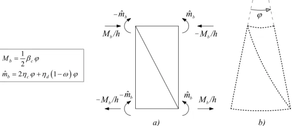
M

b

/h

M

b

/h

m

ˆ

b

m

ˆ

b

m

ˆ

b



M

b

/h

M

b

/h









a) b)

m

ˆ

b





1 2

ˆ 2 1

b c

b c d

M m



  

 

    

Figure 3: Bending principal vector force components (a) and unit cell deformed shape (b).

The anti-symmetric part of the nodal rotations





V is immediately obtained, being uncoupled from the other

components of

d

b (see eq. (9)):



6 2



₁

;

4 (2 2 ) 2

c d t d

V

c d t

    

   

  

  

 

 



The translational components

u

_V and

v

_V of

d

_V are indeterminate. The rotational components



_V and



ˆ

_V are given by the second and fourth equations of the algebraic system. These are solved by inverting the (2 2) sub-matrix of the non-zero coefficients of these equations and right-multiplying the result for the column vector formed by the second and fourth row of

f

X.

By this way, the expressions of V and ˆV are derived:



















2 2 2

2 2

1

12 2 cos 3 sin cos

2 4

2 sin 8 3 cos 2 1 ;

c

V c d t d d d d d

p

t d d c d d

 

         

      

  

  

 _   _    _

   

 

  _    _

 



















2 2 2 2

2 4 2

1 1

ˆ 12 2 sin cos 3 sin cos

2 4

cos 12 sin 24 8 3 cos 2 1 ,

V t d d c d d d d d

p

d d d d t c d d



          

        

  

  

 _  _   _

 _{  }

 

     





 _

where



_{2 4}









₂



2

cos 12 sin 24 24 12 24 12 sin 24

d d d d t c d d

p        t  d t

       

is the determinant of the coefficients matrix.

The algebraic manipulations to determine the force sub-vector

f

v are cumbersome and time-consuming and,

for brevity, they are omitted here. Besides, they are not necessary, since the transmitted shear force can be directly evaluated by analyzing the unit cell equilibrium.

The transmission mode of the axial force is finally given by the principal vector s_{a  }d fT_a, _aT_T corresponding

(11) where in place of

d

v the axial displacement vector 0 0 0 0

T u  _u _

d appears, while the force sub-vector

a

f

is obtained by substituting

d

a and

d

u in eq. (3) in place of

d

i1 and

d

i. The components of

d

a and

f

a are: •









2 2 2 # # cos 2 1 288 ,

12 cos 12 cos

si 24

0 n

d d c

t

a a

d d d d d

t a d d a u l                 _     _   _       _{ }          _          d (15)





2

2 2

4

2 2

2 cos 24 sin

2 288

sin

cos 24 sin

144 0 in 0 s 0

d d c d c d d

c t

a a

d d

d d d

t d d

a a c d u l l                                    _{ }                    f (16)

where the symbol # _{is adopted to denote indeterminate quantities. More details on the algebraic manipulations}

carried out to deduce eq. (14) and (15) are given in Appendix 2. §

Also for the X-braced girder, the eigen- and principal vectors analysis of the transmission matrix

G

can be carried out in closed form. The sub-partitions of the base cell stiffness matrix are given in the Appendix 3. Adopting the same symbolism as the Pratt girder, only the main results that will be used for the girder homogenization are here reported:

- bending transmission mode:

# 1 # 1 0 ;

2 2

1

0 0 2 3 0 ;

2

T b

T

b c c d

          _   _        _  _   d f (17)

- sectional rotational component of the shear transmission mode:















2 2 2

2 2

1

12

cos 12 sin cos

4 sin 4 3 cos 3 ,

V t d c c d d d d d

V

t d d c d d d

                      _          _

with _{48 12}



_sin4 _{12 sin}4



_

_

₁₂



_sin2



2

V t d d d d t d c t d d

 

 

  _       _

 ;

2

2 2 2 2 2

# #

cos sin sin

2 _{2 24 0 0 0 12 .}

sin sin

0 0 0 ;

T

d d d

c d d d

d

d d d d

a

a

d T

a _l

l l

u

l

  

   

 

 

 _ 



 

 _ _

   



 

 

d

f

The analysis of the components of the

f

b vectors given in eq. (14) and (17) reveals that two bending moments

are transferred through the unit cell of the Pratt and X-braced girders. The first one is generated by the axial forces acting on the nodal cross sections, the other one is due to the moments applied at the joints of the unit-cell and is induced by the bending of chords and webs. In addition, in the case of the Pratt girder unit cell, when the diagonal is eliminated or equivalently



d

 



d

0

, it results   0 . Therefore





_p



0

, and the top and bottom nodes of

the cell rotate under bending exactly of the same angle of the cross section they belong to. In other words when

0

d d



 



, the cell transfers the bending moments without deformation of the transverse webs, a result already observed in Gesualdo et al (2017b) by numerical experimentation on Vierendeel unit cells.

In both kind of examined girders, axial force is transmitted together with anti-symmetric self-equilibrated mo-ments applied at the nodes of each cell end-section. In addition, the unit cell of the Pratt girder deforms also with sectional and symmetric nodal rotations. These rotations are instead totally prevented in the X-braced girder due to symmetry of the unit cell.

2.2 Warren girder

The present approach can be also effectively adopted to analyse unit cells made up by more than one bay. To give an example we consider in this section the case of the Warren girder, whose unit cell is sketched in Figure 1c. To identify nodes and sections of the girder, we adopt a convention very similar to the one of the Pratt girder. The only difference is that here the sub-script c labels the kinematical and static quantities of the central or inner nodal section of the cell. Thus, the force and displacement vectors are respectively:

1 , 1

T T

T T T T T T

i c i i c i

   

_{ } _{ }

   

d d d d f f f f

As the Warren unit cell can be obtained by reflecting a Pratt unit cell, the stiffness matrix can be constructed starting from the one reported in Appendix 1 for the Pratt case. Furthermore, being the inner nodal section of the cell free of external load, the cell stiffness equation is:

Ξ Ξ Ξ Ξ Ξ Ξ Ξ Ξ Ξ

1 1

.

l l l c l r

i i

cl cc cr c

i _{r l r c r r} i

 

  _{ } 

  _{ } 

 _{ } 

  _{ } 

  _{ } 

  _{ } 

  _{ } 

f d

0 d

f d

(18)

The second of previous equations allows expressing

d

c as function of

d

i and

d

i1 in the form:

Ξ Ξ1 Ξ Ξ1

1

c   cc c l i cc c r i

d d d

When previous result is substituted in the first and third equation of eq. (18), the

d

c vector is eliminated and the

stiffness equation can be written as:

Ξ Ξ Ξ Ξ Ξ

Ξ Ξ Ξ Ξ Ξ

1

1

1 1

l l l r l c cc c l

i i

i _{r l r c cc c r r r} i

 

 

 

  _  _ 

 _{ } 

  _{  } 

   

  _ _ 

f d

f d (19)

the null vectors. Being the matrix symmetric, also the sum of its first and sixth rows and third and eight rows will give the null vectors. Therefore, the

A

matrix of the principal vector problem, being extracted by adding the four contiguous (5 5) sub-partitions of the condensed stiffness matrix in eq. (19), will systematically have the first and third columns and the first and third rows zero-filled. This is true also when the cell has only one bay, as the Pratt and X-braced girders of previous section. Furthermore, the

A

matrix can be viewed as the stiffness matrix of the plane elastic system obtained from the unit cell by introducing the inner constraint conditions:

1

i



i



d

d

d

and, for this reason, it is semi-positive definite. It exhibits always the following symmetric structure:

ˆ

ˆ ˆ ˆ ˆ

ˆ

0 0 0 0 0

0 0

0 0 0 0 0 .

0 0

0 0

a a a

a a a

a a a

  

  

  

 

 

 

 

 

  

 

 

 

 

 

A





   

When also the dof’s corresponding to the cell rigid longitudinal and transversal translations are constrained, the cell elastic behaviour will be totally defined by the stiffness matrix:

ˆ ˆ ˆ ˆ ˆ

ˆ a a a a a a a a a

  

  

  

 

 

 

  

 

 

 

A _

   

which is positive definite and thus invertible.

In the case of the Pratt and X-braced unit cells, the algebraic sums of the indirect stiffnesses involving an anti-symmetric nodal rotation (i.e. the out-diagonal components in the last column of

A

) are also zero, for symmetry reasons. When this happens, the antisymmetric rotation component can be determined straightforwardly being un-coupled from the other components of

d

_p. To evaluate these latter components the (2 2) sub-matrix:

ˆ

ˆ ˆ ˆ

ˆ a a

a a

 

 

 

 

  

 

 

A

must be inverted and this can be performed in closed form, hence avoiding altogether any ill-conditioning problem.

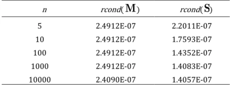
To compare the direct method with the classical one based on the

G

matrix eigen-analysis and with those proposed in Stephen and Wang (2000), a Warren unit cell with the following properties is considered:

3 2 7 4 6 4 3 2

3.5 10 1.0 10 5.0 10 2.5 10 .

c c t d d

A  mm I  mm I I  mm A  mm

The corresponding A matrix is:

11 9 9

9 9 9

9 9 10

3.4576 10 9.2485 10 4.113 . 2 10 9.2485 10 4.0989 10 4.4293 10 4.1132 10 4.4293 10 3.6657 10

 



  

 

 



  

 

 



 

A

num-From these results, it is clear that when the proposed method is adopted, the force transmission modes of the unit cell are determined by inversion of a matrix of reduced size that is well-conditioned and allows achieving the solutions with greater accuracy.

Table 1 – Warren girder force and displacement transfer matrices: reciprocals of the conditioning numbers

n rcond(

M)

rcond(

S)

5 2.4912E-07 2.2011E-07

10 2.4912E-07 1.7593E-07

100 2.4912E-07 1.4352E-07

1000 2.4912E-07 1.4083E-07

10000 2.4090E-07 1.4057E-07

3. THE EQUIVALENT CONTINUUM

As equivalent continuum, the modified polar Timoshenko beam is adopted (Ma et al. (2008), Reddy (2011)). The displacements ( , )U V of a point P x y( , ) of the beam (see Figure 4) are given by:

( ) ( ),

( ),

U u x y x

V v x



   

where u x( ) and v x( ) denote respectively the longitudinal and transversal displacements of the beam axis and ( )x

is the rotation of the cross section. The only not zero strains at P are the normal strain in the x direction: ,

x

du _yd

dx dx



  

the shear strain associated with the directions x and y: ( ),

xy dv

x dx   

and the curvature:

2

2

1 1 _,

2 4

xy

d d d v

dx dx dx

 

   _  _ 

 

where 1 2



dv dx



is the rotation of an elementary neighbourhood of P in the x-y plane.

Denoting by ( ) the cinematically admissible variations of the strain components and by



x,



xy and

m

xy

respectively the normal, tangential and the couple stress acting on the beam cross section, the virtual strain energy or internal work can be expressed as:





2

2 2

1

, 2

x x xy xy xy xy

l A

x x x xy

l

U m dAdx

d u d d v d d v

N M Q P dx

dx dx dx dx d x

     

    



   

 _{ } _ _



    

    __  __ _  __

  

 

   



, ,

x x x xy

A A

N 

_

dA Q  

_

 dA (20)

are the beam axial and shear forces, while:

and .

x x xy xy

A A

M  

_

 y dA P 

_

m dA (21)

are the Navier and polar bending moments, respectively. It is worth nothing that the dual shear deformation of

Q

_x is:

. xy

dv dx

     (22)

v'

 

v' v(x)

u(x) y

S

S'

x O

Figure 4: Kinematics of the Timoshenko beam

Under the assumption of homogeneous and isotropic linear elastic material, the stress-strain relationships are:

2

, , 2 ,

x E x xy G xy mxy G xy

        

with

E

Young modulus,

G

tangential elasticity modulus and



material length scale parameter. Substituting the previous constitutive relations in the expressions of the stress resultants, eq. (1) and (2), gives:

, ,

1

, ,

2

x xx x x Q

x xx xy xy xy

N A Q D

d

M D P S

dX

 

 _

 

  (23)

where

A

_xx and

D

_Q are respectively the axial and shear beam stiffnesses,

D

_xx



EI

is the bending stiffness, with

I

second order central moment of the beam cross section, and ₄ 2

xy

S  G A the couple stress bending stiffness. The beam equilibrium equations can be derived equating the virtual internal work



U

to the virtual work of the external loads, integrating by parts and taking into account the beam boundary conditions. For the simpler loading and constraint conditions, approximate solutions for these equations can be obtained by the Fourier series method (see ref. Reddy (2011) for more details).

ˆ ˆ ˆ

a a

a a

n n

u u

  

 (24)

where

n

ˆ

_a is the axial component of the force sub-vector

f

_a while

 

u

_a

u

ˆ

is the corresponding mean axial elongation of the unit cell.

The equivalent Navier bending stiffness



_b is calculated as the ratio of the bending moment

M

_b to the mean curvature 1/R of the cell. This latter is given by the relative rotations

 



b



of the cell end sections under

bending divided by the cell length

l

c (see Figure 3). Therefore, we have

. b c

b b

M l

M R



    (25)

Polar bending stiffness



_{p can be instead evaluated observing that, when the shear force is zero, from eq. (22)}

and (23) it follows: 2

2.

d d v

dX _dX





Hence, the polar and Navier moment of the homogenized beam make work by the same generalized strain, namely the beam curvature d

dX

 _{. For this reason, we can evaluate the polar bending stiffness as the ratio of the}

symmetric moment component of

f

b and the mean cell curvature:

ˆ

ˆ b c .

p b

m l m R



   ₍₂₆₎

The shear principal vector

s

V is coupled with the pure bending one. The shear force component

V

is given by

the subsequent condition:

ˆ

0

c b b

V l

M

m









which defines the in plane rotation equilibrium of the cell as reported in Figure 5. We recall that the displace-ment sub-vector

d

V is defined up to axial and transversal translations

u

ˆ

and v. The unit cell deformed shape due

to shear and bending is also sketched in Figure 5 assuming that these latter quantities are equal to zero. In this case, the shear angle



is equal to the average nodal section rotation  of the cell.

V/2

V/2

V/2

V/2 Mb/h

mb

Mb/h

mV 

mV 

mb mV

mV

_V _V _

MVMb

mV mb

lc

ˆ ˜

ˆ ˜

˜

˜ ˆ ˜

lc

h

Figure 5: Coupled shear and bending principal vector force component and unit cell deformed shape

Bearing in mind the components of the displacement vector

d

V and

d

V



d

b defining the deformed

configura-tions of the left and right secconfigura-tions of the cell under shear and bending, the following expression of  is easily

de-ducted: 1 2

v b

   .

Hence, the equivalent shear stiffness will be:





ˆ 2

2

b b

V

c v b

M m

V l 

  

  

 (27)

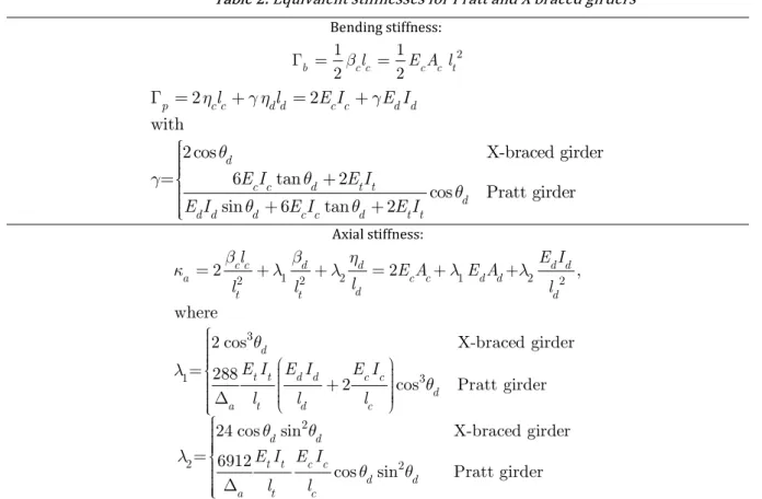
Axial and bending stiffnesses of the Pratt and X-braced girders, obtained by eq. (24), (26) and (26) and the results of sub-section 2.1, are reported in Table 2.

By inspection of these results it is deduced that Navier bending stiffnesses depend only on the chords axial stiffnesses and that, since bending of the X-braced unit cell occurs without deformation of the transvers webs, the equivalent polar bending stiffness of this girder is independent of



_t .

In addition, axial elongation of the Pratt unit cell is accompanied by rotations both of its joints and end sections. Consequently, its equivalent axial stiffness is dependent also on the bending stiffness of the chords and battens.

Table 2: Equivalent stiffnesses for Pratt and X braced girders

Bending stiffness:

2

1 1

2 2

b c cl E A lc c t

  

s

2 2

2 cos X-braced girder

6 tan 2

cos Pratt girder

6 tan 2

with

=

in

p c c d d c c d d

d

c c d t t

d

d d d c c d t t

l l E I E I

E I E I

E I E I E I

   



 

 



  

 





  

   

Axial stiffness:

1 2 1 2

2 2 2

3

1 3

2 ,

2 cos X-braced girder

288

2 cos Pratt girder

2

where

=

c d d d d

a c c d d

d

t t d

d

t t d d c c

d

c _{E A E A} E I

l

l l l

E I E I E I

l l

l

l

  

    

 



    

 _

 _

 _{ }





 

 _

 

 



The eqs. (24) - (27) completely define the elastic behaviour of the equivalent Timoshenko beam. The range of validity of these homogenized equations is analysed in the succeeding section on the basis of the numerical results of a sensitivity analysis.

5. VALIDATION STUDY

The equivalent beam model defined in Section 3, has been validated against a data set including information on the effects of the main geometrical parameters influencing the girder response. This set has been generated by f.e. solution of cantilevered and simply supported girders engendered by assembling Bernoulli-Euler beams and subjected to a unit vertical load applied respectively at the free end and at the midpoint.

The accuracy of the theoretical predictions has been quantified by the next non-dimensional measure of the homogenization error:

% 100 ,

FE

e  v v

where vFE is the vector of the vertical displacements of the girder nodal sections derived through the f.e. analysis,



v

is the vector of the variations vhomvFE, being vhom the vector of the vertical displacements of the corresponding

homogenised beam evaluated at the nodal sections of the girders.

Figure 6: Deflections of Pratt (a), X-braced (b) and Warren (c) girders.

Furthermore, to have an additional measure of accuracy and to get also direct indications about the influence exerted on the model equilibrium shapes by the couple-stress bending stiffness, for each examined girder geometry the maximum displacement f of the equivalent model is compared with that

f

FE of the corresponding f.e. model

and the one _fˆ _{of the Timoshenko (Cauchy) beam having the same bending and shear stiffness as the couple-stress} equivalent beam.

Since, as a first approximation, the main parameter influencing the relative importance of the two bending moments acting on the girder cross section is the height h of the girder, in the first set of f.e. analysis the effects of the changes of this parameter have been considered. Under the assumption that both chords and webs have the same cross section, specifically HEA100, cantilever girder f.e. models having height h=lt=300, 600 and 1200 mm, cell aspect ratios





l l

_{t c}



0.5, 1 and 2

_{and girder aspect ratio}





L l

_t



6, 12, 24 and 48

_{, being L the girder} span, have been examined. Previous values of h,  and  as well the cross sections properties were chosen to obtain

In Figure 6, as an example, the deformed shapes of f.e. girders having cell-aspect ratio





0.5

are compared with those of the corresponding equivalent beams. In Tables 3, 4 and 5 for all the considered geometries respec-tively of Pratt, X-braced and Warren girders, the homogenization errors, the equivalent stiffnesses and the deflec-tions _{, and} ˆ

FE

f f f are listed.

From these results, it can be concluded that for the whole range of considered girder heights, to have accurate estimates of the girder displacements, it is necessary to take into account the bending stiffnesses of chords and webs by means of the couple stress stiffness of the equivalent beam. Furthermore, since small values of the homog-enization error have been obtained for all the examined values of the cell shape ratio  , it is also clear that the

homogenized model is able to offer insight into the effects of this parameter on the bending response of the girders. A second series of girder models has been prepared to analyse the effects of the changes of diagonal cross-sectional area on the equivalent model accuracy, since the girder shear stiffness is strongly influenced by this geo-metric parameter. For these analysis, more stout girders under three points bending have been considered in order to highlight the shear properties effects in the girder response. For the chords of these models the standard HEA120 section has been chosen. Several back to back angles sections have been considered for the diagonals, while for the battens only the 80 x 8 back to back angle has been used.

Table 3: Pratt girders equivalent stiffnesses, deflections and homogenization errors as function of girder height and unit cell shape ratio.

α



_b



_p



_V

f

_FE f _fˆ _e%

[-] [Nmm] [Nmm] [Nmm-1_{] [mm] [mm] [mm] [-]}

h=300 mm 0.5 1.969E+13 1.740E+12 3.851E+08 5.840E-3 5.823E-₀₃ 6.356E-3 0.214 β=24 _{1 “ 1.901E+12 2.334E+08 5.810E-3}

5.791E-03 6.381E-3 0.261 2 “ 2.017E+12 1.092E+08 5.820E-3 5.791E-₀₃ 6.451E-3 0.335 h=600 mm 0.5 7.876E+13 1.740E+12 2.113E+08 1.610E-3 1.579E-₀₃ 1.648E-3 0.261 β=12 1 “ 1.901E+12 1.737E+08 1.610E-3 1.583E-₀₃ 1.663E-3 0.620 2 “ 2.017E+12 8.580E+07 1.650E-3 1.621E-₀₃ 1.748E-3 1.455 h=1200 mm 0.5 3.150E+14 1.740E+12 1.701E+08 4.680E-4 4.344E-₀₄ 4.796E-4 0.700

β=6 _{1 “ 1.901E+12 1.594E+08 4.640E-4}

4.370E-04 4.853E-4 1.723 2 “ 2.017E+12 8.014E+07 5.170E-4 4.805E-₀₃ 5.746E-4 5.003

h=300 mm 0.5 1.969E+13 2.082E+12 5.940E+08 5.557E-₀₃ 5.725E-₀₃ 6.343E-₀₃ 0.193 β=24 _{1 “ 2.456E+12 4.033E+08}

5.643E-03 5.634E-03 6.355E-03 0.212 2 “ 2.726E+12 1.974E+08 5.586E-₀₃ 5.582E-₀₃ 6.392E-₀₃ 0.091 h=600 mm 0.5 7.876E+13 2.082E+12 3.805E+08 1.574E-₀₃ 1.557E-₀₃ 1.618E-₀₃ 1.050 β=12 1 “ 2.456E+12 3.322E+08 1.554E-₀₃ 1.553E-₀₃ 1.623E-₀₃ 0.157 2 “ 2.726E+12 1.665E+08 1.563E-₀₃ 1.568E-₀₃ 1.666E-₀₃ 0.458 h=1200 mm 0,5 3.150E+14 2.082E+12 3.298E+08 4.150E-₀₄ 4.138E-₀₄ 4.386E-₀₄ 0.118

β=6 _{1 “ 2.456E+12 3.150E+08}

4.140E-04 4.143E-04 4.406E-04 0.408 2 “ 2.726E+12 1.590E+08 4.280E-₀₄ 4.359E-₀₄ 4.855E-₀₄ 2.350

The f.e. results and the predictions of the homogenised model are compared in the diagrams of Figure 7, while in Table 6 the homogenization errors and the equivalent stiffnesses are reported. In all the examined cases the model predictions have resulted to be very close to the f.e. outcomes. Thus, the homogenized model is also able to predict the shear dominated girders responses with sufficient accuracy for practical applications.

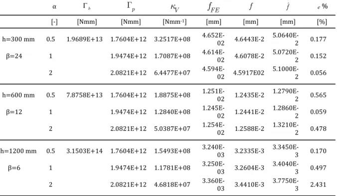
Table 5: Warren girders equivalent stiffnesses, deflections and homogenization errors as function of girder height and unit cell shape ratio.

α b



_p



_V

f

_FE f fˆ e%

[-] [Nmm] [Nmm] [Nmm-1_{] [mm] [mm] [mm] [%]}

h=300 mm 0.5 1.9689E+13 1.7604E+12 3.2517E+08 4.652E-₀₂ 4.6443E-2 5.0640E-₂ 0.177 β=24 1 1.9474E+12 1.7087E+08 4.614E-₀₂ 4.6078E-2 5.0720E-₂ 0.152 2 2.0821E+12 6.4477E+07 4.594E-₀₂ 4.5917E02 5.1000E-₂ 0.056

h=600 mm 0.5 7.8758E+13 1.7604E+12 1.8875E+08 1.251E-₀₂ 1.2435E-2 1.2790E-₂ 0.565 β=12 1 1.9474E+12 1.2840E+08 1.245E-₀₂ 1.2441E-2 1.2860E-₂ 0.059 2 2.0821E+12 5.0387E+07 1.254E-₀₂ 1.2588E-2 1.3210E-₂ 0.478

h=1200 mm 0.5 3.1503E+14 1.7604E+12 1.5493E+08 3.240E-₀₃ 3.2335E-3 3.3450E-₃ 0.170 β=6 1 1.9474E+12 1.1781E+08 3.250E-₀₃ 3.2604E-3 3.4040E-₃ 0.497 2 2.0821E+12 4.6818E+07 3.360E-₀₃ 3.4410E-3 3.7750E-₃ 2.431

Table 6: Equivalent stiffnesses, deflections and homogenization errors as function of the diagonal geometry.

diag-onal



b



p



V

f

FE f fˆ e%

[-] [Nmm] [Nmm] [Nmm-1_{] [mm] [mm] [mm] [%]}

Pratt girder 80 x 8 9.396E+13 2.702E+12 1.937E+08

L=7200 mm 70 x 7 “ 2.619E+12 1.500E+08

-9.400E-5 -9.197E05 1.068E-04 2.112 β=12 55 x 6 “ 2.548E+12 1.035E+08

-9.900E-5 -9.714E05 1.176E-04 1.571 30 x 6 “ 2.505E+12 5.787E+07

-1.130E-4 -1.100E04 1.450E-04 2.021 X-braced girder 80 x 8 9.396E+13 2.918E+12 3.787E+08

-8.500E-5 -8.481E05 9.226E-05 0.763 L=7200 mm 70 x 7 “ 2.744E+12 2.910E+08 -8.600E-5 -8.633E05 9.513E-05 0.669 β=12 55 x 6 “ 2.598E+12 1.979E+08 -8.900E-5 -8.923E05 1.009E-04 0.668 30 x 6 “ 2.512E+12 1.067E+08 -9.700E-₅ -9.668E05 1.165E-_{04 0.424}

Warren girder 80 x 8 9.396E+13 2.708E+12 1.441E+08 -6.660E-4 -6.675E04 7.120E-04 0.243 L=14400 mm 70 x 7 “ 2.621E+12 1.187E+08 -6.720E-4 -6.732E04 7.227E-04 0.193 β=12 55 x 6 “ 2.548E+12 8.792E+07 -6.830E-4 -6.839E04 7.439E-04 0.211 30 x 6 “ 2.505E+12 5.298E+07 -7.110E-₄ -7.100E04 7.979E-_{04 0.105}

Figure 7: Deflections of Pratt (a), X-braced (b) and Warren (c) girders

6. CONCLUSION

A new procedure for homogenizing large repetitive beam-like structures is presented. Such a method is based on the analysis of the eigen- and principal vectors of the transfer state matrix of the unit cell. As a substitute medium, a Timoshenko polar beam is adopted. Differently from the approaches until now proposed, the polar character of the equivalent beam is not deduced by kinematical conjectures nor inspired by the micro-structure: it is a direct consequence of the pattern of the inner forces acting in the lattice when the pure bending mode of the cell is active. The main advantage of the presented method is that it allows to operate directly on the sub-partitions of the unit cell stiffness matrix. For the simpler unit cells, as those of the Pratt and X braced girders, the method leads to closed form solutions for force transmission modes, that are then used to determine the stiffnesses of the corre-sponding equivalent beam. When the unit cell instead has a complex geometry and its transmission modes can be determined only numerically, it is shown that the method we propose has a very low computational cost, since the search of the transmission modes, reduces to the inversion of a (3 3) stiffness matrix, and has a higher accuracy, being this (3 3) matrix well-conditioned.

2017a). Its range of validity is bounded by the hypothesis of linear elasticity. Further research will thus be needed to extend the proposed method also in the elasto-plastic range whereas the response of the unit cell has to be ana-lysed by approximated methods as those reported in Fraldi et al. (2010, 2014) and Cennamo et al. (2017).

References

Bacigalupo, A., Gambarotta, L., 2014. Homogenization of periodic hexa-and tetrachiral cellular solids, Composite Structures, 116:461-476.

Bakhvalov, N., Panasenko, G., 1989. Averaging processes in periodic media: mathematical problems in the mechan-ics of composite material, Kluwer Academic.

Bazant, Z., Christensen, M., 1972. Analogy between micropolar continuum and grid frameworks under initial stress, International Journal of Solids and Structures, 8(3):327–346.

Cao, J., Grenestedt, J.L., Maroun, W.J., 2007. Steel truss/composite skin hybrid ship hull. Part I: design and analysis, Composites Part A: Applied Science and Manufacturing, 38(7):1755-1762.

Cennamo, C., Gesualdo, A., Monaco, M., 2017. Shear plastic constitutive behaviour for near-fault ground motion, ASCE Jounal of Engineering Mechanics, 143(9):04017086.

Cheng, B., Qian, Q., Sun, H., 2013. Steel truss bridges with welded box-section members and bowknot integral joints, Part I: linear and non-linear analysis, Journal of Constructional Steel Research, 80:465-474.

De Iorio, A., Grasso, M., Penta, F., Pucillo, G.P., Pinto, P., Rossi, S., Testa, M., Farneti, G., 2014a. Transverse strength of railway tracks: Part 1. Planning and experimental setup, Frattura ed Integrità Strutturale, 30:478-485.

De Iorio, A., Grasso, M., Penta, F., Pucillo, G.P., Rosiello, V., 2014b. Transverse strength of railway tracks: Part 2. Test system for ballast resistance in line measurement, Frattura ed Integrità Strutturale, 30:578-592.

De Iorio, A., Grasso, M., Penta, F., Pucillo, G.P., Rosiello, V., Lisi, S., Rossi, S., Testa, M., 2014c. Transverse strength of railway tracks: Part 3. Multiple scenarios test field, Frattura ed Integrita Strutturale, 30:593-601.

De Iorio, A., Grasso, M., Penta, F., Pucillo, G.P., Rossi, S., Testa, M., 2017. On the ballast–sleeper interaction in the longitudinal and lateral directions, Proceedings of the Institution of Mechanical Engineers, Part F: Journal of Rail and Rapid Transit, doi: https://doi.org/10.1177/0954409716682629.

Dos Reis, F., Ganghoffer, J.F., 2012. Construction of micropolar continua from the asymptotic homogenization of beam lattices, Computers and Structures, 112:354-363.

El Khoury, E., Messager, T., Cartraud, P., 2011. Derivation of the young's and shear moduli of single-walled carbon nanotubes through a computational homogenization approach, International Journal for Multiscale Computational Engineering, 9(1):97-118.

Fillep, S., Mergheim, J., Steinmann, P., 2014. Microscale modeling and homogenization of rope-like textiles, PAMM - Proceedings in Applied Mathematics and Mechanics, 14(1):549-550.

Fraldi, M., Gesualdo, A., Guarracino, F., 2014. Influence of actual plastic hinge placement on the behavior of ductile frames, Journal of Zhejiang University-Science A, 15(7):482-495.