Lat. Am. j. solids struct. vol.10 número3

(1)

Abs tract

A study on the finite element (FE) analysis of laminated compo-site plates is described in this paper. In order to investigate struc-tural behavior of laminated composite plates, a four-node lami-nated plate element is newly developed by using a higher order shear deformation theory (HSDT). In particular, assumed natural strains are introduced in the present FE formulation to alleviate the locking phenomenon. Several numerical examples are carried out and its results are then compared with the existing reference solutions. It is found to be that the proposed FE is very effective to remove the locking phenomenon and produces reliable numeri-cal solutions for most laminated composite plate structures.

Key words

Laminate Composite Plate, Finite Element, Higher Order Shear Deformation, Locking Phenomenon, Assumed Strain Method

FE analysis of laminated composite plates using a

higher order shear deformation theory with assumed

strains

1 INTRODUCTION

Laminated composite plates have been extensively used in many engineering disciplines such as civil engineering, marine engineering and aerospace engineering due to its high strength to weight ratio and excellent corrosion resistance. With the growing use of laminated composite material, it be-comes very important to conduct numerical analysis and to use the resulting information in the structural design process. This situation clearly has demanded the development of efficient and accurate numerical analysis techniques which are necessarily required to predict the behaviors of laminated plates.

In the early days, classical laminated plate theory (CLPT) has been mainly used with negligence of the effect of transverse shear deformation. However, due to the increasing use of thick laminated plate in construction, thick plate theories such as the first order shear deformation theory (FSDT) and the higher order shear deformation theory (HSDT) are needed to take into account transverse

Sa ng Jin L e e* an d H a Ryon g Ki m

ADOPT Research Group, Department of Architectural Engineering, Gyeongsang Na-tional University, Republic of Korea

Received 01 Mar 2012 In revised form 05 Aug 2012

(2)

Latin American Journal of Solids and Structures 10(2013) 523 – 547

shear deformation through the thickness direction of the plates. In particular, The HSDTs do not required shear correction factor and it can generally guarantee zero transverse shear stress values on the top and bottom surfaces of the plate. Some important and early works on HSDT can be found in the open literatures [1-5] where more realistic representation of transverse shear deformation were generally tried to be provided. Later, Zhang and Yang [6] described some recent developments of the FEs based on various laminated composite plate theories. Reddy [1] suggested a simple but very useful HSDT for laminated composite plates. His version of HSDT is based on equivalent single layer plate theory and it allows parabolic variation of transverse shear stress and also satisfies zero shear stress boundary conditions at the top and bottom surfaces of the plate. Moreover, it does not involve any unknown fields which do not have any physical meaning. Bose and Reddy [7, 8] ana-lyzed laminated plates by using a unified third-order laminate plate theory that contains classical, first-order and third-order theories and they presented analytical method using the Navier and Levy equations and the FE method using the unified third order laminate plate theory. A review on the various methods used in the estimation of transverse and inter-laminar stresses for laminated com-posite plates and shell including both analytical and numerical methods was provided by Kant and Swaminathan [9]. Kant and Manjunatha [10] provided the FE based on HSDT having twelve de-grees of freedom per node. They presented three-dimensional stress and strain states to investigate the flexure-membrane coupling behavior of unsymmetrical laminated plate. Akhars and Li [11] de-veloped a spline finite strip method for static and free vibration analysis of composite plates using Reddy’s HSDT. Pervez et al [12] developed a two dimensional serendipity FE based on a refined HSDT having seven degrees of freedom per node to perform the linear static analysis of laminated orthotropic composite plates. Latheswary et al [13] studied the behavior of laminated composite plates under static loading by using a four-node nonconforming element based on HSDT. Goswami [14] presented a simple C^0 FE formulation for nine-node FE with six degrees of freedom based on HSDT.

(3)

2 REVIEWS ON HSDT

2.1 Displacement definition

The total domain (Ω) of laminated plate consists of the mid_-surface and the thickness as shown in Figure 1 and it can be defined as

Ω = x

1,x2,x3

(

)

x

1,x2

(

)

∈_Ω

0, x3∈ − h

2, h

2 ⎡

⎣ ⎢ ⎢

⎤

⎦ ⎥ ⎥ ⎧

⎨ ⎪ ⎪

⎩ ⎪ ⎪

⎫ ⎬ ⎪ ⎪

⎭ ⎪

⎪ (1)

where is the xy-plane and h is denoted as thickness of plate.

In order to represent the shape of transverse shear deformation in realistic way, the displacement fields may include higher order terms as follows [1]

u

1

(

x1,x2,x3

)

=u1

(

x1,x2

)

+x3θ2+c1x3 3 _θ

2+

∂u

3

∂x

1 ⎛

⎝ ⎜⎜ ⎜⎜

⎞

⎠ ⎟⎟ ⎟⎟

(2) u

2

(

x1,x2,x3

)

=u2

(

x1,x2

)

−x3θ1+c1x3 3 ₋_θ

1+ ∂u

3 ∂x

2 ⎛

⎝ ⎜⎜ ⎜⎜

⎞

⎠ ⎟⎟ ⎟⎟

u

(4)

Figure 1 Geometry and sign convention of laminated composite plate

2.2 Strain definition

The strains in the plate are defined by linear strain-displacement relationship as follows

ε ij =

1 2

∂u_j ∂x_i +

∂u_i ∂x_j ⎛ ⎝ ⎜⎜ ⎜⎜ ⎞ ⎠ ⎟⎟ ⎟⎟⎟=1

2

(

uj,i +ui,j

)

(3)

Substituting (2) into (3) yields

ε p

{ }

= ε₁ ε₂ γ₁₂ ⎧ ⎨ ⎪⎪ ⎪⎪ ⎩ ⎪⎪ ⎪⎪ ⎫ ⎬ ⎪⎪ ⎪⎪ ⎭ ⎪⎪ ⎪⎪ = ε₁( )0

ε₂( )0

γ₁₂( )0 ⎧ ⎨ ⎪⎪ ⎪⎪⎪ ⎩ ⎪⎪ ⎪⎪ ⎪ ⎫ ⎬ ⎪⎪ ⎪⎪⎪ ⎭ ⎪⎪ ⎪⎪ ⎪ +x 3

ε₁( )1

ε₂( )1

γ₁₂( )1 ⎧ ⎨ ⎪⎪ ⎪⎪⎪ ⎩ ⎪⎪ ⎪⎪ ⎪ ⎫ ⎬ ⎪⎪ ⎪⎪⎪ ⎭ ⎪⎪ ⎪⎪ ⎪ +c

1

( )

x3 3

ε₁( )3

ε₂( )3

γ₁₂( )3 ⎧ ⎨ ⎪⎪ ⎪⎪⎪ ⎩ ⎪⎪ ⎪⎪ ⎪ ⎫ ⎬ ⎪⎪ ⎪⎪⎪ ⎭ ⎪⎪ ⎪⎪ ⎪

=

{

ε( )0

}

+x

x3

2 γ

= u 1,1 u 2,2 u

1,2+u2,1

⎧ ⎨ ⎪⎪ ⎪⎪⎪ ⎩ ⎪⎪ ⎪⎪ ⎪ ⎫ ⎬ ⎪⎪ ⎪⎪⎪ ⎭ ⎪⎪ ⎪⎪ ⎪

,

{ }

ε( )1 =

θ_2,1

−θ_1,2

θ_2,2−θ_1,1 ⎧ ⎨ ⎪⎪ ⎪⎪⎪ ⎩ ⎪⎪ ⎪⎪ ⎪ ⎫ ⎬ ⎪⎪ ⎪⎪⎪ ⎭ ⎪⎪ ⎪⎪ ⎪

,

_,1 ⎧ ⎨ ⎪⎪ ⎪⎪ ⎪⎪ ⎩ ⎪⎪ ⎪⎪ ⎪⎪ ⎫ ⎬ ⎪⎪ ⎪⎪ ⎪⎪ ⎭ ⎪⎪ ⎪⎪ ⎪⎪ ,

γ( )0

{

}

=

θ₂+u

3,1

−θ₁+u

3,2 ⎧ ⎨ ⎪⎪⎪ ⎩ ⎪⎪ ⎪ ⎫ ⎬ ⎪⎪⎪ ⎭ ⎪⎪ ⎪

,

{

γ( )2

}

=

θ₂+u

3,1

−θ₁+u

3,2 ⎧ ⎨ ⎪⎪⎪ ⎩ ⎪⎪ ⎪ ⎫ ⎬ ⎪⎪⎪ ⎭ ⎪⎪ ⎪ . (5)

2.3 Constitutive equation

In this study, each layer of laminate plate is assumed as orthotropic material and the normal

transverse stress ₍σ

3') is assumed to be negligible. Therefore, the constitutive equation for the k

th

layer with respect to the material coordinate system x 1

'_,_x 2 '_,_x

3 '

(

)

can be written as

σ'

{ }

(k) =⎡C

⎣ ⎤⎦ (k)

ε'

{ }

(k)

σ₁'

σ₂'

τ₁₂'

τ₁₃'

τ₂₃' ⎧ ⎨ ⎪⎪ ⎪⎪ ⎪⎪ ⎪⎪⎪ ⎩ ⎪⎪ ⎪⎪ ⎪⎪ ⎪⎪ ⎪ ⎫ ⎬ ⎪⎪ ⎪⎪ ⎪⎪ ⎪⎪⎪ ⎭ ⎪⎪ ⎪⎪ ⎪⎪ ⎪⎪ ⎪

(k₎

=

C

11 C12 0 0 0

C

21 C22 0 0 0

0 0 C

33 0 0

0 0 0 C

44 0

0 0 0 0 C

55 ⎡ ⎣ ⎢ ⎢ ⎢ ⎢ ⎢ ⎢ ⎢ ⎢ ⎢ ⎢ ⎤ ⎦ ⎥ ⎥ ⎥ ⎥ ⎥ ⎥ ⎥ ⎥ ⎥ ⎥

(k) ε₁'

ε₂'

γ₁₂'

γ₁₃'

γ₂₃' ⎧ ⎨ ⎪⎪ ⎪⎪ ⎪⎪ ⎪⎪⎪ ⎩ ⎪⎪ ⎪⎪ ⎪⎪ ⎪⎪ ⎪ ⎫ ⎬ ⎪⎪ ⎪⎪ ⎪⎪ ⎪⎪⎪ ⎭ ⎪⎪ ⎪⎪ ⎪⎪ ⎪⎪ ⎪ (k₎

(6)

in which _C

ij are the components of rigidity matrix for the k

th

layer as follows

C 11=

E 1

'

1−_ν 12 ' ν21 ' , C 22 = E 2 '

1−_ν 12 ' ν21 ' , C 12= ν21 ' _E 1 '

1−_ν 12

'

ν21 ' =C21,

C

33 =G12 ' _,_C

44 =G13 ' _,_C

55=G23 '

(7)

where _E

1'

,

E2' are the Young’s modulus in

' ' 1, 2

x x direction respectively, G

12'

,

G13 '

_,

_G

23

' _{are the}

shear modulus and _ν

(6)

If the angle ϑ _{between the material coordinate system} x

1'

( )

and the global coordinate system

is once determined as shown in Figure 1, the transformation can be possible between two coord i-nate systems.

Therefore, stresses and strains {σ_}, {ε_} in global coordinate system can be obtained by using the transformation matrix ⎡_T

⎣ ⎤⎦ and stresses and strains {σ'}, {ε'} in material coordinate system:

σ

{ }

= ⎡_⎣T⎤_⎦

{ }

σ' ,

{ }

ε ₌ ⎡_T

⎣ ⎤⎦

{ }

ε' (8)

where the transformation matrix ⎡_T

⎣ ⎤⎦ between material coordinate system and global coordinate system can be written as

T ⎡ ⎣ ⎤⎦ =

c2 s2 ₋2sc 0 0

s2 c2 2sc 0 0

sc ₋sc c2

−s2 ₀ ₀

0 0 0 c ₋s

0 0 0 s c

⎡ ⎣ ⎢ ⎢ ⎢ ⎢ ⎢ ⎢ ⎢ ⎢ ⎤ ⎦ ⎥ ⎥ ⎥ ⎥ ⎥ ⎥ ⎥ ⎥ (9)

where c =cosϑ and s =sinϑ in which ϑ is the fiber’s angle as shown in Figure 1.

N₁ M₁ P₁

N₂ M₂ P₂

N₁₂ M₁₂ P₁₂ ⎡ ⎣ ⎢ ⎢ ⎢ ⎢ ⎢ ⎤ ⎦ ⎥ ⎥ ⎥ ⎥ ⎥ =

k=1 nlayer

∑

x₃k

x₃k+1

∫

σ 1 σ 2 τ 12 ⎧ ⎨ ⎪⎪ ⎪⎪⎪ ⎩ ⎪⎪ ⎪⎪⎪ ⎫ ⎬ ⎪⎪ ⎪⎪⎪ ⎭ ⎪⎪ ⎪⎪⎪

1 x₃

( )

x₃ 3

{

}

dx₃,

Q₁₃ R₁₃

Q₂₃ R₂₃ ⎡ ⎣ ⎢ ⎢ ⎢ ⎤ ⎦ ⎥ ⎥ ⎥ = _k₌₁

nlayer

∑

x₃k

x₃k+1

∫

τ13

τ 23 ⎧ ⎨ ⎪⎪⎪ ⎩ ⎪⎪⎪ ⎫ ⎬ ⎪⎪⎪ ⎭

⎪⎪⎪ 1

( )

x3 2

{

}

dx₃

(7)

Latin American Journal of Solids and Structures 10(2013) 523 – 547 where _nlayer _{is the number of layers in laminated plate.}

The above stress resultant terms can be rewritten in the matrix form:

N

{ }

M

{ }

P

{ }

⎧ ⎨ ⎪⎪ ⎪⎪⎪ ⎩ ⎪⎪ ⎪⎪ ⎪ ⎫ ⎬ ⎪⎪ ⎪⎪⎪ ⎭ ⎪⎪ ⎪⎪ ⎪ = A ⎡

⎣ ⎤⎦ ⎡⎣B⎤⎦ c1⎡⎣E⎤⎦

B ⎡

⎣ ⎤⎦ ⎡⎣D⎤⎦ c1⎡_⎣F⎤_⎦

E ⎡

⎣ ⎤⎦ ⎡⎣F⎤⎦ c1⎡⎣H⎤⎦

⎡ ⎣ ⎢ ⎢ ⎢ ⎢ ⎢ ⎢ ⎤ ⎦ ⎥ ⎥ ⎥ ⎥ ⎥ ⎥

⎡

⎣ ⎤⎦ c2⎡⎣T⎤⎦

⎡ ⎣ ⎢ ⎢ ⎢ ⎤ ⎦ ⎥ ⎥ ⎥

γ( )0

{ }

γ( )2

{ }

⎧ ⎨ ⎪⎪ ⎪⎪ ⎩ ⎪⎪ ⎪⎪ ⎫ ⎬ ⎪⎪ ⎪⎪ ⎭ ⎪⎪ ⎪⎪ (12)

Where _{the components of the rigidity matrices}_A

ij, Bij, Dij, Eij, Fij, Hij, G_ij, S_ij, T_ij can be

written as follows

A_ij,B_ij,D_ij,E_ij,F_ij,H_ij

(

)

=

∑

,

G_ij,S_ij,T_ij

(

)

=

x₃k x₃k+1

∫

⎡_⎣⎢Q_ijk⎤_⎦⎥

(

1,

( )

x₃ 2,

( )

x₃ 4

)

dx₃ k=1

nlayer

∑

(13)

and the above equation can be explicitly rewritten in the following form:

A_ij = Q_ijk x₃k+1₋_x 3 k

(

)

=G_ij

k=1 nlayer

∑

,

B_ij = 1

2 Qij

k _x

3 k+1

(

)

2− _x

3 k

( )

2

{

}

k=1 nlayer

∑

,

D_ij = 1

3 Qij

k _x

3 k+1

(

)

3−

( )

x₃k 3

{

}

k=1 nlayer

∑

=S_ij ,

E_ij = 1

4 Qij

k _x

3 k+1

(

)

4− _x

3 k

( )

4

{

}

k=1 nlayer

∑

,

F_ij = 1

5 Qij

k _x

3 k+1

(

)

5−

( )

x₃k 5

{

}

k=1 nlayer

∑

=T_ij ,

H_ij = 1

7 Qij

k _x

3 k+1

(

)

7− _x

3 k

( )

7

{

}

k=1 nlayer

∑

.

(8)

3 FINITE ELEMENT FORMULATION

3.1 Kinematics and displacement field

In this study, a four_{-node plate element having seven degrees of freedom per node is formulated}

using the isoparametric formulation. Therefore the geometry and displacement fields of the pr e-sent FE can be defined in the following form:

x

i = a=1

4

∑

N

axi a

(

i ₌_{1, 3}

)

_,

u

i = a=1

4

∑

N

aui a

(

i₌_{1, 7}

)

(15)

where N

a is the bilinear Lagrange shape function associatedwith node a, xi is the position ve c-tor of the plate and the nodal displacement vecc-tor u_ia ₌

{ }

ua _{has seven components such as}

ua

{ }

= u

1

a

,u

2

a

,u

3

a

,θ 1

a

,θ 2

a

,∂u3

a

∂x

1 ,∂u3

a

∂x

2 ⎧

⎨ ⎪ ⎪

⎩ ⎪ ⎪

⎫ ⎬ ⎪ ⎪

⎭ ⎪

⎪ (16)

where ∂u 3 a

/∂x 1, ∂u3

a /∂x

2 are two additional degrees of freedom related to the higher order terms of (2) which do not appear in the FE based on the FSDT.

3.2 Strain_-displacement relationship matrix

Using (15), the strains of (4) can be rewritten in the form of the strain-displacement relation m a-trix as follows

ε_p

{ }

= B0

a

⎡

⎣⎢ ⎤⎦⎥+ B1 a

⎡

⎣⎢ ⎤⎦⎥+c1

( )

x3 3

B2 a

⎡ ⎣⎢ ⎤⎦⎥

(

)

{ }

ua

a=1 4

∑

γ_s

{ }

= ⎡B₃a

⎣⎢ ⎤⎦⎥+c2

( )

x3 2

B₄a

⎡ ⎣⎢ ⎤⎦⎥

(

)

{ }

ua

a=1 4

∑

(17₎

(9)

Latin American Journal of Solids and Structures 10(2013) 523 – 547 B 0 a ⎡ ⎣⎢ ⎤ ⎦⎥ = ∂N a ∂x 1

0 0 0 0 0 0

0 ∂Na ∂x

2

0 0 0 0 0

∂N a ∂x 2 ∂N a ∂x 1

0 0 0 0 0 ⎡ ⎣ ⎢ ⎢ ⎢ ⎢ ⎢ ⎢ ⎢ ⎢ ⎢ ⎢ ⎢ ⎢ ⎤ ⎦ ⎥ ⎥ ⎥ ⎥ ⎥ ⎥ ⎥ ⎥ ⎥ ⎥ ⎥ ⎥ , B 1 a ⎡ ⎣⎢ ⎤ ⎦⎥=

0 0 0 0 ∂Na

∂x 1

0 0

0 0 0 −∂Na ∂x

2

0 0 0

0 0 0 −∂Na ∂x 1 ∂N a ∂x 2 0 0 ⎡ ⎣ ⎢ ⎢ ⎢ ⎢ ⎢ ⎢ ⎢ ⎢ ⎢ ⎢ ⎢ ⎢ ⎤ ⎦ ⎥ ⎥ ⎥ ⎥ ⎥ ⎥ ⎥ ⎥ ⎥ ⎥ ⎥ ⎥ , B 2 a ⎡ ⎣⎢ ⎤ ⎦⎥=

0 0 0 0 ∂Na

∂x 1 ∂N a ∂x 1 0

0 0 0 −∂Na ∂x

2

0 0 ∂Na

∂x 2

0 0 0 −∂Na ∂x 1 ∂N a ∂x 2 ∂N a ∂x 2 ∂N a ∂x 1 ⎡ ⎣ ⎢ ⎢ ⎢ ⎢ ⎢ ⎢ ⎢ ⎢ ⎢ ⎢ ⎢ ⎢ ⎤ ⎦ ⎥ ⎥ ⎥ ⎥ ⎥ ⎥ ⎥ ⎥ ⎥ ⎥ ⎥ ⎥ , B 3 a ⎡ ⎣⎢ ⎤ ⎦⎥ =

0 0 ∂Na ∂x

1

0 N

a 0 0

0 0 ∂Na ∂x

2 −N

a 0 0 0

⎡ ⎣ ⎢ ⎢ ⎢ ⎢ ⎢ ⎢ ⎢ ⎤ ⎦ ⎥ ⎥ ⎥ ⎥ ⎥ ⎥ ⎥ , B 4 a ⎡ ⎣⎢ ⎤ ⎦⎥ =

0 0 0 0 N

a Na 0 0 0 0 −N

a 0 0 Na

⎡ ⎣ ⎢ ⎢ ⎢ ⎤ ⎦ ⎥ ⎥ ⎥.

3.3 Total potential energy of plate

The total potential energy of the laminated plate can be written by using the stress resultants and the corresponding strains as follows

Π =1

2 dA

∫

{ }

N T

{ }

ε( )0 +

{ }

M T

{ }

ε( )1 +c1

{ }

P

T ε( )3

{ }

+

{ }

Q T

{ }

γ( )0 +c2

{ }

R

T γ( )2

{ }

(

)

dA−P (18)

In the _{discretized FE domain, total potential energy can be written as}

Π = 1 2

{ }

u

T

K_N ⎡

⎣ ⎤⎦+⎡_⎣KM⎤_⎦+⎡_⎣KP⎤_⎦+⎡_⎣⎢KQ⎤_⎦⎥+⎡_⎣KR⎤_⎦

(

)

{ }

u −

{ }

u T

{ }

f (19)

f is the global vector of nodal forces with typical

nodal force sub_-vector for node a

{ }

_fa ₌ _f

u₁ a_,_f

u₂ a_,_f

u₃ a_,_f

θ 1

a_,_f θ

2

a_,_f

∂u₃/∂x₁

a _,_f

∂u₃/∂x₂ a

{

}

and ⎡_K

⎣ ⎤⎦ is the

global stiffness matrix where

K ⎡

⎣ ⎤⎦= nel∧ e₌1

K(e) ⎡

⎣⎢ ⎤⎦⎥ (20)

where ∧ nel e₌1

[] is the finite element assembly operator and the element stiffness matrix is divided into

five contributions

K( )e ⎡

⎣⎢ ⎤⎦⎥= KN e ( ) ⎡

⎣⎢ ⎤⎦⎥+ KM e ( ) ⎡

⎣⎢ ⎤⎦⎥+ KP e ( ) ⎡

⎣⎢ ⎤⎦⎥+ KQ e ( ) ⎡

⎣⎢ ⎤⎦⎥+ KR e ( ) ⎡

⎣⎢ ⎤⎦⎥ (22)

in which _K N (e) ⎡

⎣⎢ ⎤⎦⎥, KM (e) ⎡

⎣⎢ ⎤⎦⎥, KP (e) ⎡

⎣⎢ ⎤⎦⎥, KQ (e) ⎡

⎣⎢ ⎤⎦⎥ and KR (e) ⎡

⎣⎢ ⎤⎦⎥ are

K_N(e) ⎡

⎣⎢ ⎤⎦⎥= dA(e)

∫

⎛⎡_⎣⎢Ba₀⎤_⎦⎥T ⎡_⎣A⎤_⎦⎡_⎣⎢Bb₀_⎦⎥⎤+_⎣⎢⎡B₁a⎤_⎦⎥T⎡_⎣B_⎦⎤⎡_⎣⎢B₀b⎤_⎦⎥+c₁⎡_⎣⎢B₂a⎤_⎦⎥T⎡_⎣E⎤_⎦⎡_⎣⎢B₀b⎤_⎦⎥ ⎝

⎜⎜⎜ ⎞_⎠⎟⎟⎟dA ,

K_M(e) ⎡

⎣⎢ ⎤⎦⎥= dA(e)

∫

⎛⎡_⎣⎢Ba₀⎤_⎦⎥T ⎡_⎣B⎤_⎦⎡_⎣⎢B₁b_⎦⎥⎤+_⎣⎢⎡B₁a⎤_⎦⎥T⎡_⎣D_⎦⎤⎡_⎣⎢B₁b⎤_⎦⎥+c₁⎡_⎣⎢B₂a⎤_⎦⎥T ⎡_⎣F⎤_⎦⎡_⎣⎢B₁b⎤_⎦⎥ ⎝

⎜⎜⎜ ⎞_⎠⎟⎟⎟dA ,

K_P(e) ⎡

⎣⎢ ⎤⎦⎥= dA(e)

∫

⎛c₁⎡_⎣⎢Ba₀_⎦⎥⎤T⎡_⎣E⎤_⎦_⎣⎢⎡Bb₂_⎦⎥⎤+c₁⎡_⎣⎢B₁a⎤_⎦⎥T_⎣⎡F_⎦⎤⎡_⎣⎢B₂b⎤_⎦⎥+c₁2_⎣⎢⎡B₂a_⎦⎥⎤T ⎡_⎣H_⎦⎤⎡_⎣⎢B₂b⎤_⎦⎥ ⎝

⎜⎜⎜ ⎞_⎠⎟⎟⎟dA ,

K_Q(e) ⎡

⎣⎢ ⎤⎦⎥= dA(e)

∫

⎛⎡_⎣⎢Ba₃_⎦⎥⎤T ⎡_⎣G_⎦⎤⎡_⎣⎢B₃b⎤_⎦⎥+c₂⎡_⎣⎢Ba₄_⎦⎥⎤T_⎣⎡S⎤_⎦⎡_⎣⎢B₃b⎤_⎦⎥ ⎝

⎜⎜⎜ ⎞_⎠⎟⎟⎟dA ,

K_R(e)

⎡

⎣⎢ ⎤⎦⎥= dA

∫

(e)

c₂⎡B₃a ⎣⎢ ⎤⎦⎥

T S ⎡ ⎣ ⎤⎦ B4

b ⎡

⎣⎢ ⎤⎦⎥+c2 2 _B 4 a ⎡ ⎣⎢ ⎤⎦⎥ T T ⎡ ⎣ ⎤⎦ B4

b ⎡ ⎣⎢ ⎤⎦⎥ ⎛

⎝

⎜⎜⎜ ⎞_⎠⎟⎟⎟dA .

(23)

3.4 Substitute strain_{-displacement}matrix via assumed strain method

In this study, the assumed strain method is employed to alleviate the possible locking phenom

e-non. Therefore, assumed strains are derived by using the interpolation functions based on L a-grangian polynomial and the strain values at the sampling points where the locking does not e

x-ist.

For natural assumed transverse shear strains _γ 13

0 ( )_{( )}A

and _γ 23

0 ( )_{( )}A

, the following sampling

(11)

Latin American Journal of Solids and Structures 10(2013) 523 – 547 

γ₁₃( )0( )A →_(0,1)

1: (0,−1)2, γ23 0

( )( )A _→_{(1, 0)}

1: (−1, 0)2. (24)

Using (24), the assumed natural strains can be defined in the following form:



γ₁₃( )0( ) =A

a=1 2

∑

P_δ

( )

ξ₂ _γ

13

δ_,_γ_

23 0 ( )( ) =A

a=1 2

∑

Q_δ

( )

ξ₁ _γ

23

δ

(25)

where δ _{denotes the position of the sampling point as shown in Figure 2 and the interpolation}

functions _P_,

Q are employed as follows

P₁= 1

2

(

1+ξ2

)

, P2= 1 2 1

−ξ₂

(

)

,

Q₁ =1

2

(

1+ξ1

)

, Q2= 1 2 1

−ξ₁

(

)

.

(26)

Figure 2 The position of sampling point; (left) γ13

0

( )( )A _{and (right)}_γ_ 23

0 ( )( )A

Transverse shear strain_{-displacement relationship produced by assumed strain method can be} written in the following matrix form:

γs

{ }

=

a₌1 4

∑

B

3 a A_{( )} ⎡ ⎣⎢

⎤

⎦⎥+c2

( )

x3 2

B 4 a ⎡ ⎣⎢

⎤ ⎦⎥

(

)

{ }

ua ₍₂₇₎

where B

3

(12)

Latin American Journal of Solids and Structures 10(2013) 523 – 547 B

3 a₍A₎ ⎡

⎣⎢ ⎤⎦⎥= 1 4

0 0 Ξ₁ α₁Ξ₂+β₁Ξ₃ α₂Ξ₂+β₂Ξ₃ 0 0 0 0 Ξ₄ γ₁Ξ₅+β₁Ξ₆ γ₂Ξ₅+β₂Ξ₆ 0 0 ⎡ ⎣ ⎢ ⎢ ⎢ ⎤ ⎦ ⎥ ⎥ ⎥ (28)

in which the Ξ

1, Ξ2,Ξ3,Ξ4, Ξ5,Ξ6,αi, βi, γi are

Ξ₁ =1 4ξ1

a ₁₊_ξ 2 a_ξ

2

i 3₋_x

i 4

(

)

, β _i =1

4 xi 1₋_x

i 2₊_x

i 3₋_x

i 4

(

)

, γ_i =1

4( −_x

i 1₋_x

i 2₊_x

i 3₊_x

i 4₎

(29)

where _x i a

,ξ_ia _{are the coordinates of nodal point}_a _{in global coordinate system and natural coo}

r-dinate system respectively.

3.5Substitute element stiffness matrix for transverse shear

In previous section, the assumed strains are defined in natural coordinate system and so tran s-verse shear rigidity matrix of (13) can be also defined in the natural coordinate system as follows



G_ij ₌ ∂ξi ∂_x

α ∂ξ_j

∂_x β

G_αβ,



S_ijQ ₌ ∂ξi ∂_x

α

S_αj, S_ijS ₌ ∂ξ_j

∂_x β

S_iβ .

(30)

Consequently, transverse shear stiffness terms of (23) can be rewritten as follows

K_Q(e) ⎡

⎣⎢ ⎤⎦⎥= dA

∫

⎡B₃( )A

⎣⎢ ⎤⎦⎥ T

 G ⎡ ⎣ ⎤⎦ B3

A ( ) ⎡

⎣⎢ ⎤⎦⎥+c2⎡⎣B4⎤⎦ T _

SQ ⎡

⎣⎢ ⎤⎦⎥ B3 A ( ) ⎡ ⎣⎢ ⎤⎦⎥ ⎛ ⎝ ⎜⎜ ⎜ ⎞ ⎠ ⎟⎟⎟⎟dA,

K_R(e) ⎡

⎣⎢ ⎤⎦⎥= dA

∫

c₂⎡B₃( )A ⎣⎢ ⎤⎦⎥

T  SS ⎡

⎣⎢ ⎤⎦⎥⎡⎣B4⎤⎦+c22⎡⎣B4⎤⎦ T

T ⎡ ⎣ ⎤⎦⎡⎣B4⎤⎦ ⎛ ⎝ ⎜⎜ ⎜ ⎞ ⎠ ⎟⎟⎟⎟dA.

(31)

In this study, (31) will be used instead of the terms ⎡K_Q(e)

⎣⎢ ⎤⎦⎥ and KR (e) ⎡

(13)

Latin American Journal of Solids and Structures 10(2013) 523 – 547 4 NUMERICAL EXAMPLES

In order to investigate the accuracy and reliability of the newly developed laminated plate el e-ment HSA4, a series of numerical test for symmetric and unsymmetric laminated plates are co n-sidered. The square plates with the simply supported boundary conditions are used in the test. More specifically, two sets of boundary conditions, SS1 and SS₂ _{are employed in numerical tests}

as follows

SS_{1 :}u

1 =0, u3 =0,θ2=0, ∂u

3 ∂x

1

=0 at x

2 =0, x2=a ,

u

2= 0, u3 =0,θ1=0, ∂u

3 ∂x

2

=0 at x

1 =0, x1=a ,

SS_{2 :}u

2 =0, u3=0,θ2=0, ∂u

3 ∂x

1

=0 at x

2 =0, x2 =a ,

u

1=0, u3 =0,θ1=0, ∂u

3 ∂x

2

=0 at x

1= 0, x1=a

(32)

and the three sets of material properties are used as follows

M1 : E₁/E₂= 25.0, G₁₂ =G₁₃ =0.5E₂,G₂₃ =0.2E₂,ν12 =0.25, M2 : E₁/E₂= 40.0, G₁₂ =G₁₃ =0.6E₂,G₂₃= 0.5E₂,ν12 =0.25,

M3 : Facesheets : E₁=19×₁₀6_,_E

2=1.5×106,G12 =G13 =1×106,

G₂₃ =0.9×₁₀6_,_ν

12=ν13 =0.22,ν23 =0.49,

Core isotropic

(

)

:E =1×₁₀3_,G ₌₅×₁₀2_,_ν ₌_{0.0 .}

(33)

In this study, the laminated plates are also assumed to be subjected to sinusoidal load or un i-form load as follows

L1=q x

qa4 ⎛

⎝ ⎜⎜ ⎜⎜

⎞

⎠ ⎟⎟ ⎟⎟⎟, σ

1=σ1 h2

qa2 ⎛

⎝ ⎜⎜ ⎜⎜

⎞

⎠ ⎟⎟ ⎟⎟⎟, σ

2=σ2 h2

qa2 ⎛

⎝ ⎜⎜ ⎜⎜

⎞

⎠ ⎟⎟ ⎟⎟⎟,

τ

12 =τ12 h2

qa2 ⎛

⎝ ⎜⎜ ⎜⎜

⎞

⎠ ⎟⎟ ⎟⎟⎟, τ

13 =τ13 h

qa2 ⎛

⎝ ⎜⎜ ⎜⎜

⎞

⎠ ⎟⎟

⎟⎟, τ23 =τ23 h

qa2 ⎛

⎝ ⎜⎜ ⎜⎜

⎞

⎠ ⎟⎟ ⎟⎟.

(14)

Note that the deflection w is calculated at the center of the plate and the stresses are pr

o-duced at the nearest Gauss point to the following locations

u 3:

a

2, a

2, 0 ⎛ ⎝ ⎜⎜ ⎜

⎞ ⎠ ⎟⎟ ⎟⎟, σ1:

a

2, a

2,± h

2 ⎛

⎝ ⎜⎜ ⎜

⎞ ⎠ ⎟⎟ ⎟⎟, σ2:

a

2, a

2,± h

2 ⎛

⎝ ⎜⎜ ⎜

⎞ ⎠ ⎟⎟ ⎟⎟,

τ

12 : 0, 0,± h

2 ⎛ ⎝ ⎜⎜ ⎜

⎞ ⎠ ⎟⎟

⎟⎟, τ13 : 0, a

2, 0 ⎛ ⎝ ⎜⎜ ⎜

⎞ ⎠ ⎟⎟ ⎟⎟, τ23:

a

2, 0, 0 ⎛ ⎝ ⎜⎜ ⎜

⎞ ⎠ ⎟⎟ ⎟⎟

(36)

where a is the width of the plate and h is the thickness of the plate.

It should be noted that Reddy’s displacement function definition of (2) can reserve zero shear stress boundary condition at the top and bottom of the laminated plate but this condition cannot be reserved anymore when assumed strain method is adopted with the HSDT. Therefore, the following modified strain definition is used when we calculate transverse shear stress value t o-gether with (10):

γs

{ }

= B

3 a A_{( )} ⎡ ⎣⎢

⎤

⎦⎥+c2

( )

x3 2

B 3 a A_{( )} ⎡ ⎣⎢

⎤ ⎦⎥

(

)

{ }

ua

a=1 4

∑

, where c₂ =4 / h2_.

(37)

With (37), we can enforce the values of γs to zero at top (x

3=h/ 2) and bottom (x3 =−h/ 2) of laminated plates and eventually the zero shear stress values can be achieved at the top and bottom of the plates.

4.1 Symmetric cross-ply(0°/ 90°/ 90°/ 0°)square laminated plate

(a) Convergence rate test: A four_-layer symmetric cross-ply (0°/ 90°/ 90°/ 0°) laminated co m-posite plate is analyzed to check the convergence rate of the present FE (HSA4) and its perfor-mance for the variation of thickness values. In this test, material property, boundary condition and load case such as M_1, SS_1, L₁ are used. Five cases with ₄×₄_,8×8_, ₁₂×₁₂_,16×16 and

32×32 _{FE meshes are employed in the test. Two aspect ratios}a_/h ₌₁₀_{, 100} are used in FE

(15)

Latin American Journal of Solids and Structures 10(2013) 523 – 547 Figure 3 _{The convergence test results of the present FE (HSA4) for}a_/h₌₁₀and 100.

The present plate element shows _{a good convergence rate. In particular, we can see that the} present FE solution _{has a good agreement with the elasticity solution [19] and}achieves a certain level of convergence with the case of 16×16 _{FE mesh for both thin and thick plates. We ther} e-fore decided to use the 16×16 FE mesh with 256 four_-_{node elements for numerical test throug} h-out this study. Note that FE reference solution [14] was produced by a nine-node plate elementso that the reference solution with _n×_n _{FE mesh is compared to the present solution with the}

(16)

Table _{1 Convergence test of a simply supported (}_SS1_{) symmetric cross}_-_{ply (}₀_°_{/ 90}_°_{/ 90}_°_{/ 0}_°_{) laminated plate under sinusoidal} transverse load₍a_/h₌₁₀_).

Solution Mesh Size _w σ σ

2 τ12 τ13 τ23

Present

4×₄

0.6975 0.4691 0.3336 0.0231 0.2318 0.1392

Present* _- 0.5001 0.3556 0.0246 0.2471 0.1483

Goswami[14] 0.7286 0.5714 0.3172 0.0266 0.1977 0.0978

Present

8×8

0.7147 0.5367 0.3759 0.0262 0.2701 0.1540

Present* _- 0.5454 0.3820 0.0266 0.2745 0.1565

Goswami[14] 0.7274 0.5683 0.3287 0.0275 0.2642 0.1014

Present

12×₁₂

0.7179 0.5500 0.3842 0.0268 0.2779 0.1569

Present* _- 0.5541 0.3871 0.0270 2800 0.1581

Goswami[14] 0.7261 0.5626 0.3266 0.0272 0.2993 0.1188

Present

16×16

0.7190 0.5547 0.3872 0.0270 0.2807 0.1580

Present* _- 0.5570 0.3888 0.0271 0.2818 0.1586

Goswami[14] 0.7250 0.5591 0.3244 0.0269 0.3169 0.1231

Present

32×32 0.7200 0.5593 0.3901 0.0272 0.2834 0.1590

Present* _- 0.5599 0.3905 0.0273 0.2837 0.1591

Elasticity[19] - 0.7430 0.5590 0.4010 0.0275 0.3010 0.1960

Note_{: Present*: Stresses are extrapolated}_{from Gauss point to the point of (36).}

Table _{2 Convergence test of a simply supported (}_SS₁_{) symmetric cross}_-ply₍₀_°_{/ 90}_°_{/ 90}_°_{/ 0}_°_{) laminated plate under sinusoidal} transverse load₍a_/h₌₁₀₀_).

Solution Mesh Size _w σ σ

2 τ12 τ13 τ23

Present

4×₄

0.4124 0.4556 0.2291 0.0181 0.2575 0.1000

Present* _- 0.4856 0.2442 0.0192 0.2745 0.1063

Goswami[14] 0.4366 0.5430 0.2422 0.0201 0.1859 0.0912

Present

8×8

0.4291 0.5170 0.2599 0.0205 0.2997 0.1112

Present* _- 0.5254 0.2641 0.0208 0.3046 0.1130

Goswami[14] 0.4354 0.5458 0.2464 0.0203 0.2022 0.1288

Present

12×₁₂

0.4320 0.5291 0.2659 0.0210 0.3083 0.1134

Present* _- 0.5329 0.2679 0.0211 0.3106 0.1143

Goswami[14] 0.4347 0.5421 0.2451 0.0202 0.2210 0.1356

Present

16×16

0.4331 0.5333 0.2681 0.0211 0.3114 0.1142

Present* _- 0.5355 0.2692 0.0212 0.3127 0.1147

Goswami[14] 0.4343 0.5352 0.2432 0.0200 0.2291 0.1414

Present

32×32 0.4340 0.5375 0.2702 0.0213 0.3144 0.1150

Present* _- 0.5380 0.2704 0.0213 0.3147 0.1151

Elasticity[19] - 0.4347 0.5390 0.2760 0.0216 0.3370 0.1410 Note_{: Present*: Stresses are extrapolated from Gauss point to the point of (36).}

(17)

Latin American Journal of Solids and Structures 10(2013) 523 – 547 stresses of the plate are summarized in Table 3 and it is compared with the solutions produced by elasticity solution [19], Reddy [1], Akhras and Li [11] and Pervez et al [12]. It is found to be that both the present FE HAS4 and the standard FE HSD4 have a good agreement with reference

solutions for thick plate situations such as a_/h ₌₄ and 10_{. However, if the aspect ratio becomes}

a larger value, i.e. the plate becomes thin, the four node standard plate element HSD4 has some discrepancies with reference solutions. Specifically, for the aspect ratio a_/h₌₁₀₀_{, the HSD4 has}

around 50% of error compare to the reference solutions. It can be considered as the evidence that

HSD4 exhibits the shear locking phenomenon when the plate becomes thinner. However, the pr e-sent plate element alleviates the shear locking phenomenon very effectively with full integration and enhances its performance in great manner as shown in Table3. We provide the distributions of in_{-plane stresses}σ

1,σ2 and transverse shear stresses τ13,τ23, through the thickness direction in Figures 4-7 for a_/h ₌_{10 and 100}_.

Table 3 The non_-dimensionalized _{deflection and stresses of a simply supported}₍_SS₁₎_{symmetric cross-}_ply (0°/ 90°/ 90°/ 0°) laminated plate under sinusoidal transverse load.

a_/h _Theory

w σ σ₂ τ₁₂ τ13 τ23

4

Present(HSA4) 1.9014 0.6973 0.6245 0.0456 0.2112 0.2439 HSD4 1.8997 0.6965 0.6225 0.0455 0.2114 0.2430 Elasticity[19] 1.9540 0.7200 0.6630 0.0467 0.2190 0.2920

Reddy[1] 1.8937 0.6651 0.6322 0.0440 0.2064 0.2389

Aknas and Li [11] 1.8941 0.6800 0.6338 0.0444 0.2064 0.2390

Pervez et al [12] 1.8910 0.7180 0.6420 0.0467 0.2090 0.2410

10

Present(HSA4) 0.7090 0.5547 0.3872 0.0270 0.2807 0.1580

HSD4 0.7122 0.5482 0.3824 0.0267 0.2782 0.1540

Elasticity[19] 0.7430 0.5590 0.4010 0.0275 0.3010 0.4960

Reddy[1] 0.7147 0.5456 0.3888 0.0268 0.26040 0.1531

Aknas and Li [11] 0.7149 0.5576 0.3896 0.0270 0.2642 0.1530 Pervez et al [12] 0.7190 0.5700 0.3970 0.0276 0.2780 0.1570

20

Present(HSA4) 0.5065 0.5379 0.3021 0.0227 0.3028 0.1267

HSD4 0.4877 0.5164 0.2900 0.0218 0.2900 0.1150

Elasticity[19] 0.5170 0.5430 0.2080 0.0230 0.3280 0.1560

Reddy[1] 0.5060 0.5393 0.3043 0.0228 0.2825 0.1234

Aknas and Li [11] 0.5061 0.5513 0.3053 0.0230 0.2829 0.1226

Pervez et al [12] 0.5080 0.5520 0.3090 0.0232 0.2990 0.1260

100

Present(HSA4) 0.4331 0.5333 0.2681 0.0211 0.3114 0.1142

HSD4 0.2215 0.2720 0.1367 0.0108 0.1267 _-0.0228

Elasticity[19] 0.4347 0.5390 0.2760 0.0216 0.3370 0.1410

Reddy[1] 0.4343 0.5387 0.2708 0.0213 0.2897 0.1117

Aknas and Li [11] 0.4345 0.5508 0.2765 0.0215 0.2947 0.1076

Pervez et al [12] 0.4340 0.5460 0.2740 0.0216 0.3070 0.1170

(18)

Latin American Journal of Solids and Structures 10(2013) 523 – 547 Figure₄Variation of the in_-plane stress(σ

1)through the thickness direction (z/h) of a simply supported( SS1)cross-ply

(0°/ 90°/ 90°/ 0°) laminated composite plate under sinusoidal transverse load (a_/h₌₄ and 100₎

Figure 5 Variation of the in-plane stress(σ

(19)

Latin American Journal of Solids and Structures 10(2013) 523 – 547 Figure 6 Variation of the transverse shear stress₍τ

13)through the thickness direction (z/h)of a simply supported (SS1)

cross_-ply₍_0°_{/ 90°}_{/ 90°}_{/ 0°}₎_{laminated composite plate under sinusoidal transverse load (}a_/h₌₄ and 100₎

Figure7 Variation of the transverse shear stress₍τ

(20)

The stress values produced by the present HSA4 have also good agreements with reference solution for in_-_{plane stress}�

! and transverse shear stress τ13. However, the standard FE HSD4 has a huge discrepancy with the present solution for thin plate with the aspect ratio a_/h₌₁₀₀_.

From d_i_{rect comparison between the present solution and the solution produced by the standard}

FE, we can identify the locking disappear in the present solution. We here provide numerical results for a_/h ₌₁₀₀ as _{a benchmark solution for future study since the stress distributions pr}

o-duced by a FE based on HSDT is few in literatures.

4.2 Unsymmetric cross-ply (_0°_{/ 90°})square laminated plate

This example is used to investigate the performance of the present FE HSA4 on the analysis of

unsymmetric composite plate. A two-layer unsymmetric cross-ply (_{0 / 90º}) laminated plate is

analyzed in the test. The material property, boundary condition and load case such as M_1,SS_1,L₁ _{are used. The central deflection and stresses are calculated for four aspect ratios}

=

/

4, 10, 20, 100

a

h

and summarized in Table 4.

Table ₄The non_{-dimensionalized deflection and stresses of a simply supported (}_SS₁₎_{unsymmetric cross}_-ply₍

0 / 90º)laminated plate under sinusoidal transverse load.

/

a

h

_Theory w σ

1 σ2 τ12

5

Present(HSA4) 1.6836 _-0.7847 0.7847 _-0.0540

Elasticity[19] 1.7287 _-0.7723 0.8036 _-0.0586

HSDT *[9] 1.6800 _-0.7510 0.7720 _-0.0557

HSDT **[9] 1.7037 _-0.7662 0.7662 _-0.0572

Reddy[1] 1.6760 _-0.8385 0.8385 _-0.0558

Latheswary et al [13] - - - -

10

Present(HSA4) 1.2168 _-0.7228 0.7228 _-0.0525

Elasticity[19] 1.2318 _-0.7317 0.7353 _-0.0540

HSDT *[9] 1.2192 _-0.7269 0.7273 _-0.0533

HSDT **[9] 1.2274 _-0.7286 0.7286 _-0.0539

Reddy[1] 1.2161 _-0.7468 0.7468 _-0.0533

Latheswary et al [13] 1.2161 0.7517 0.7517 0.0532

20

Present(HAS4) 1.0995 _-0.7136 0.7136 _-0.0521

Elasticity[19] 1.1060 _-0.7200 0.7206 _-0.0529

HSDT *[9] 1.1025 _-0.7189 0.7186 _-0.0527

HSDT **[9] 1.1078 _-0.7185 0.7185 _-0.0530

Reddy[1] 1.1018 _-0.7235 0.7235 _-0.0527

Latheswary et al [13] - - - -

100

Present(HSA4) 1.0619 _-0.7087 0.7087 _-0.0520

Elasticity[19] 1.0742 _-0.7219 0.7219 _-0.0529

HSDT*[9] 1.0651 _-0.7161 0.7161 _-0.0525

HSDT**[9] 1.0695 _-0.7152 0.7152 _-0.0527

Reddy[1] 1.0651 _-0.7161 0.7161 _-0.0525

(21)

Latin American Journal of Solids and Structures 10(2013) 523 – 547 The numerical results are compared with the exact elasticity solution [19], analytical solutions [2, 8] and the FE solution [20]. In this example, we found that the present solutions have good agreements with the reference solutions regardless of aspect ratios. In specific, stress values are

reasonably accurate for all aspect ratios

a

_/

h

=

_{4, 10, 20, 100}

_.

4.3 Unsymmetric angle-ply (⎡_⎣⎢45°/−45°⎤_⎦⎥_n) square laminated plate

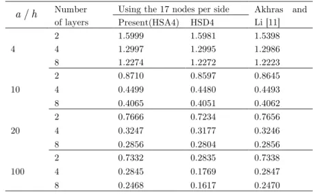
(a) Uniform load (_L2): The unsymmetric angle-ply (⎡_⎣45°/−45°⎤_⎦_n) laminated plate are analyzed with four aspect ratios a_/h ₌_{4, 10, 20, 100} _{with three different numbers of layers such as n=2,}

4, 8. Material properties, boundary condition and load case are used as M2, SS2, L2 respectively.

The numerical results are non_-dimensionalized and summarized in Table 5. From numerical r

e-sults, both the present HSA4 and the standard HSD4 have _{good agreements with reference sol}

u-tion_{[9] for the aspect ratio}a_/h ₌₄_._{However, for the aspect ratio}

a

_/

h

=

₁₀₀

the standard FE

HSD4 shows a great discrepancy with the reference solution although it exhibit reasonably good

performance up to a_/h ₌₂₀_{. However, the pr}_{esent FE HSA4 does not show any shear locking}

phenomenon for thin angle-ply unsymmetric laminated plate. In this section, we also investigate the effect of differ_{ent of layer number on the central deflection with the assumption that}_plates

keepthe same total thickness value. From numerical result, when we double the number of layers from n=2 to n=4, the center deflection is reduced up to 60% in case of the aspect ratio a_/h ₌₁₀₀ _{and 25 % for aspect ratio}a_/h ₌ ₄ _{respectively. In other words, thick laminated}

plate is very sensitive to variation of the number of layers than thin laminated plate. We also

found that the increase _{of the number of layers in laminated plate generally tends to reduce the}

deflection of_{laminated plate when the plate has the same thickness value.}

Table 5 The non_-_{dimensionalized deflection of a simply supported (}_SS₁₎_{unsymmetric angle-}_{ply (}⎡_{45° / -45°}

⎣ ⎤⎦4) laminated plate

under uniform load.

a_/h Number

of layers

U_{sing the 17 nodes per side} Akhras and Li [11]

Present(HSA4) HSD4

4

2 1.5999 1.5981 1.5398

4 1.2997 1.2995 1.2986

8 1.2274 1.2272 1.2223

10

2 0.8710 0.8597 0.8645

4 0.4499 0.4480 0.4493 8 0.4065 0.4051 0.4062

20

2 0.7666 0.7234 0.7656

4 0.3247 0.3177 0.3246

8 0.2856 0.2804 0.2856

100

2 0.7332 0.2835 0.7338

4 0.2845 0.1769 0.2847

(22)

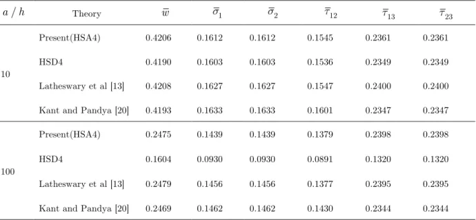
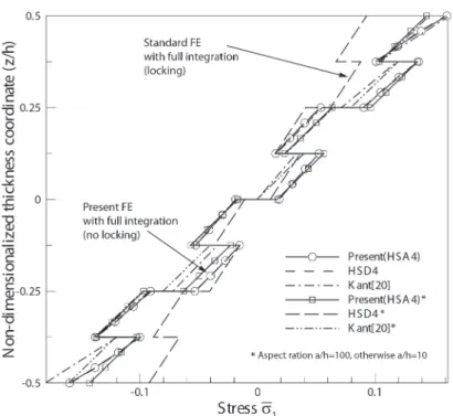
(b) Sinusoidal_{load (}_L₁₎_{: I}_{n this example, the analysis of}_{unsymmetric angle}_{-ply (}⎡_45°_/_−45°

⎣ ⎤⎦4)

laminated plate is carried out with two aspect ratios a / h=10, 100 and sinusoidal load. This

example provides the results of more detailed investigation on the performance of the present FE

HSA4 for unsymmetric angle-ply plate. Material properties, boundary condition and load case are

used as M_1,SS_2,L₁res_pectively._The non_-dimensionalized deflection and stresses are summarized in Table 6. From numerical results, the HSA4 has excellent agreements with the reference

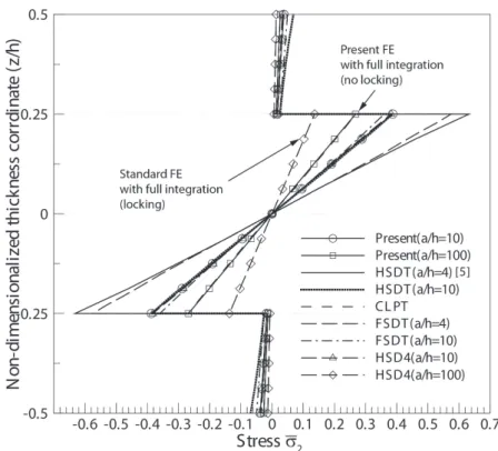
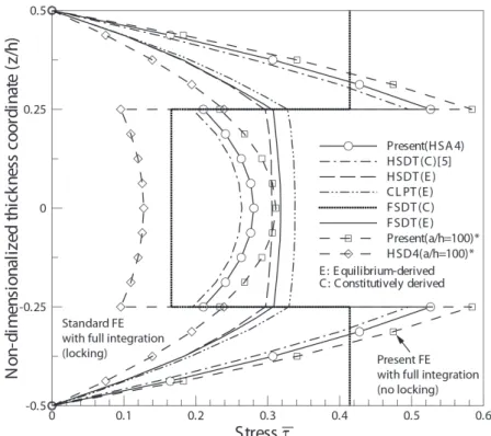
solu-tions [10, 13]. However, the standard FE HSD4 has the error of 35% compared to the reference solutions for aspect ratio a / h=100. Figures 8 and 9 show the variation of non-dimensionalized in-plane stress σ

1 and transverse shear stress τ13 through the thickness direction for the aspect

ratios _{a / h}₌_{10 and 100}_{. In particular, the present element HSA4 can produce a good parabolic}

shape than that of HSD4 for the transverse shear stress τ

13 as shown in Figures 8 and 9. The

present FE shows also a good performance to predict the maximum stress value of in-plane stress

σ

1 and transverse shear stress τ13.

Table 6 The non_{-dimensionalized deflection of a simply supported}₍_SS2_{) unsymmetric angle}_{-ply (}⎡_{45° / -45°}

⎣ ⎤⎦4) laminated plate under sinusoidal transverse load.

a_/h _Theory w σ

1 σ2 τ12 τ13 τ23

10

Present(HSA4) 0.4206 0.1612 0.1612 0.1545 0.2361 0.2361

HSD4 0.4190 0.1603 0.1603 0.1536 0.2349 0.2349

Latheswary et al [13] 0.4208 0.1627 0.1627 0.1547 0.2400 0.2400

Kant and Pandya [20] 0.4193 0.1633 0.1633 0.1601 0.2347 0.2347

100

Present(HSA4) 0.2475 0.1439 0.1439 0.1379 0.2398 0.2398

HSD4 0.1604 0.0930 0.0930 0.0891 0.1320 0.1320

Latheswary et al [13] 0.2479 0.1456 0.1456 0.1377 0.2395 0.2395

(23)

Latin American Journal of Solids and Structures 10(2013) 523 – 547 Figure 8 Variation of the in_{-plane stress}₍σ

1) through the thickness (z/h) of a simply supported �� unsymmetric angle-ply (⎡_⎣45° / -45°⎤_⎦

4) laminated composite plate under sinusoidal transverse load (a / h = 10 and 100)

Figure 9 Variation of transverse shear stress₍τ

13)through the thickness(z/h) of a simply supported �� unsymmetric

(24)

4.4 Unsymmetric cross-ply (0°/ 90°/ core / 0°/ 90°) square sandwich plate

The analysis of a five-layer unsymmetric and unbalanced sandwich plate with isotropic core is carried out and its numerical results are presented. Material properties, boundary condition and load case are used as M_3,SS_1,L₁_{respectively.}_T_{he thickness of core is equal to total thickness of}

four face sheets which have all the same thickness_{. T}he non_-dimensionalized deflection and in -plane stresses are summarized in Table 7. From numerical results, both HSD4 and HSA4 have a good agreements with the reference _{solutions up to the aspect ratio} _{a / h}₌₁₀_{. For the aspect}

ratio _{a / h}₌₁₀₀_{, the present element HSA4 have approximately the 1}_-8 % of differences with

reference solutions [1, 21] but the standard HSD4 have almost the 60 % of difference with the

reference soluti_{ons because of locking phenomenon.}

Table 7 The non_-_{dimensionalized deflection and stresses of a simply supported}��_{unsymmetric cross}_-_ply

(0°/ 90°/ core / 0°/ 90°) sandwich plate under sinusoidal transverse load.

/

a

h

_Theory _w σ

1 σ2 τ12

4

Present(HSA4) 12.9278 _-1.4673 1.4673 0.1970

HSD4 13.2060 _-1.4773 1.4773 0.1992

HSDT*[9] 14.1627 _-1.6445 1.4931 0.2031

HSDT**[9] 14.3440 _-1.5328 1.5328 0.2196

Reddy[1] 8.7941 _-0.9937 0.9937 0.1291

10

Present(HSA4) 3.0264 _-0.7504 0.7504 0.0874

HSD4 3.0260 _-0.7310 0.7310 0.0855

HSDT*[9] 3.3032 _-0.8140 0.7606 0.0946

HSDT**[9] 3.3197 _-0.7771 0.7771 0.0951

Reddy[1] 2.3075 _-0.6815 0.6815 0.0787

100

Present(HSA4) 1.0105 _-0.6029 0.6029 0.0649

HSD4 0.4306 _-0.2558 0.2558 0.0275

HSDT*[9] 1.0697 _-0.6231 0.6226 0.0691

HSDT**[9] 1.0763 _-0.6216 0.6216 0.0696

Reddy[1] 1.0595 _-0.6214 0.6214 0.0690

5 CONCLUSIONS

A four_{-node laminated composite plate element having seven degrees freedom per node is newly}

developed by using the HSDT and assumed strains to perform the FE stress analysis. The acc u-racy and reliability of new laminated composite plate element is thoroughly tested by using five

numerical _{tests for both symmetric and}_unsymmetric _{situations. From numerical results, the pr}

(25)

AcknowledgementsThe research grants from _{the Ministry of Construction & Transportation, Korea,}

for the Construction Technology Research & Development Program (PN: 06-R&D_-_{B03) are grat} e-fully acknowledged.

References

[1] Reddy JN. A simple Higher order Theory for laminated composite plates. ASME J Appl Mech 1984;51:745-752.

[2] Bert CW_. _{A critical evaluation of new plate theories applied to laminated composites}_._ComposStruct

1984;2:329-347.

[3] Lo_KH_{, Christensen}_RM,Wu _EM. _{A high-order theory of plate deformation-part 2: laminated plates. Appl} Mech 1977_;_44:669_-676_.

[4] Reddy JN. A review of the literature on finite element analysis of progressive failure in laminated composite plates. Shock Vib Digest 1985;17(4):3-8.

[5] Reddy JN. Mechanics of laminated composite plate. CRC Press, 1997.

[6] Zhang YX, Yang CH. Recent developments in finite element analysis for laminated composite plates. Co

m-pos Struct 2009_;88_:147_-157.

[7] Bose P, Reddy JN. Analysis of composite plates using various plate theories. Part 1: Formulation and an a-lytical solutions. Struct Engng Mech 1998;6(6):583-612.

[8] Bose P, Reddy JN. Analysis of composite plates usingvarious plate theories. Part 2: Finite element model and nume_{rical results. Struct Engng Mech 1998;6(7):727}_-746.

[9] Kant T, Swaminathan K. Estimation of transverse/interlaminar stresses in laminated composites-a selective review and survey of current developments. Compos Struct 2000_;49_:65_-75_.

[10] Kant T, Manjunatha BS. An unsummetric FRClaminate C0_{finite element model with 12 degrees of freedom}

per node. Eng Comput 1988;5:300-308.

[11] Akhras G, Li W. Static and free vibration analysis of composite plates using splinefinite strips with higher

order shear deformation. Compos Part B: Eng 2005;36:496-503.

[12] Pervez T, Seibi AC, Al-Jahwari FKS. _{Analysis of thick orthotropic laminated composite plates based on}

higher order shear deformation theory. Compos Struct 2005_;71:414_-_422.

[13] Latheswary S, Valasrajan KV, Rao YVKS. Behavior of laminated composite plates using higher order shear

deformation theory. IE(I) J-AS 2004;85:10-17.

[14] Goswami S. A C0 _{plate bending element with refined shear deformation theory for composite structures.}

Compos Struct 2006_;72_:375_-382.

[15] Lee SJ, Kim HR. Finite element a_{nalysis of}s_{ymmetric and}u_nsymmetric_laminated _platesbased on _h_igher

order shear deformation t_heory_._I_n:_{Proceedings of}Autumn _{Congress of Architectural Institute of Korea,} Cheongju, 26-27 Oct 2007.p. 249-252.

[16] Nayak AK, Moy SSJ, Shenoi RA. Free vibration analysis of composite sandwich plates based on Reddy’s

higher –order theory. Compos Part B: Eng 2002;33:505-519.

[17] Nayak AK, Shenoi RA. Assumed strain finite elements for buckling and vibration analysis of initially

stressed damped composite sandwich plates. Sandwi Struct and Mater 2005;7:307-334.

[18] Lee SJ. Free_{-vibration analysis of plates by using a four node finite element formulated with assumed nat}

u-ral transverse shear strain. J Sound Vibration 2004;278:657-684.

[19] Pango NJ. Exact solutions for rectangular bidirectional composites and sandwich plates. J Compos Mater

1970;4:20-34.

[20] Kant T, Pandya BN. A simple finite element formulation of a higher order theory of unsymmetrically lam

i-nated composite plates. Compos Struct 1988_;9_:215_-246_.

[21] Kant T, Swaminathan K. Analytical solutions for the static analysis of laminated composite and sandwich

(26)