www.hydrol-earth-syst-sci.net/15/3367/2011/ doi:10.5194/hess-15-3367-2011
© Author(s) 2011. CC Attribution 3.0 License.
Earth System
Sciences
Evaluating uncertainty estimates in hydrologic models:
borrowing measures from the forecast verification community
K. J. Franz1and T. S. Hogue2
1Department of Geological and Atmospheric Sciences, Iowa State University, Ames, IA 50011, USA
2Department of Civil and Environmental Engineering, University of California, Los Angeles, CA, 90095, USA Received: 17 March 2011 – Published in Hydrol. Earth Syst. Sci. Discuss.: 30 March 2011
Revised: 20 October 2011 – Accepted: 29 October 2011 – Published: 15 November 2011
Abstract. The hydrologic community is generally moving towards the use of probabilistic estimates of streamflow, pri-marily through the implementation of Ensemble Streamflow Prediction (ESP) systems, ensemble data assimilation meth-ods, or multi-modeling platforms. However, evaluation of probabilistic outputs has not necessarily kept pace with en-semble generation. Much of the modeling community is still performing model evaluation using standard determinis-tic measures, such as error, correlation, or bias, typically ap-plied to the ensemble mean or median. Probabilistic forecast verification methods have been well developed, particularly in the atmospheric sciences, yet few have been adopted for evaluating uncertainty estimates in hydrologic model simu-lations. In the current paper, we overview existing proba-bilistic forecast verification methods and apply the methods to evaluate and compare model ensembles produced from two different parameter uncertainty estimation methods: the Generalized Uncertainty Likelihood Estimator (GLUE), and the Shuffle Complex Evolution Metropolis (SCEM). Model ensembles are generated for the National Weather Service SACramento Soil Moisture Accounting (SAC-SMA) model for 12 forecast basins located in the Southeastern United States. We evaluate the model ensembles using relevant metrics in the following categories: distribution, correla-tion, accuracy, conditional statistics, and categorical statis-tics. We show that the presented probabilistic metrics are easily adapted to model simulation ensembles and provide a robust analysis of model performance associated with param-eter uncertainty. Application of these methods requires no information in addition to what is already available as part of traditional model validation methodology and considers the entire ensemble or uncertainty range in the approach.
Correspondence to:K. J. Franz ([email protected])
1 Introduction
In the classic definition, forecast verification is the process of assessing the skill of a forecast or set of forecasts (Murphy and Winkler, 1987; Jolliffe and Stephenson, 2003; Wilks, 2006). Verification methods have been well developed in the atmospheric sciences (Jolliffe and Stephenson, 2003; Wilks, 2006) and their application to hydrologic forecasts has been progressing in recent years, particularly for probabilistic ver-ification (Franz et al., 2003; Bradley et al., 2004; Verbunt et al., 2006; Laio and Tamea, 2007; Bartholmes et al., 2009; Renner et al., 2009; Brown et al., 2010; Demargne et al., 2010; Randrianasolo et al., 2010). One of the earliest at-tempts at verification was published by Finley (1884) who undertook an evaluation of the success of tornadoes fore-casts. His early (and controversial) work sparked interest and a range of alternative methods in probabilistic verification, many of which are in use today (Murphy, 1997). Notable early verification papers in atmospheric and meteorological sciences have since included Cooke (1906) who undertook one of the first extensive verification studies, Ramsey (1926) and de Finetti (1937) who undertook early work in subjective probability theory, Murphy (1966) who overviewed proba-bilistic predictions and decision making, and Murphy and Epstein (1967) where the authors provided an overview of early development in probabilistic predictions and summa-rized terminology and definitions in the field.
verification, including: evaluating thevalueof predictions, evaluating theskill of predictions, performing quality con-trolon the forecast, and finally, investigating the cause(s) of predictionerrors.
Model evaluation is not dissimilar from forecast verifica-tion, except that the approach is generally aimed at evaluat-ing the reproduction of historical events rather than the pre-diction of future events. However, the goals of forecast ver-ification and model evaluation (i.e. verver-ification) are analo-gous. Hydrologists are interested in thevalue andskill of their simulations, as well as the potential sources of error in their modeling system (Muleta and Nicklow, 2005; Beven, 2006; Gupta et al., 2006; Clark and Kavetski, 2010; Kavet-ski and Clark, 2010; Schoups et al., 2010). Despite the solid existence of probabilistic verification measures in the atmo-spheric and meteorological sciences, few metrics are rou-tinely applied by the hydrologic community. Historically, evaluation of hydrologic models ensembles has been under-taken with standard deterministic measures, such as error, correlation, or bias, typically applied to the ensemble mean or median and occasionally application of a containing ratio metric (Xiong and O’Connor, 2008). While creating a de-terministic variable simplifies the corresponding model eval-uation, deterministic evaluation measures are deficient for fully analyzing probabilistic forecast or model performance (Franz et al., 2003; Bradley et al., 2004; Demargne et al., 2010). The recent growth of probabilistic streamflow esti-mates in hydrologic modeling, including ensemble data as-similation methods (Kitanidis and Bras, 1980a,b; Evensen, 1994; Margulis et al., 2002; Seo et al., 2003, 2009), multi-modeling platforms (Ajami et al., 2007; Duan et al., 2007; Vrugt and Robinson, 2007; Franz et al., 2010), Ensemble Streamflow Prediction (ESP) and other probabilistic fore-casting systems (Day, 1985; Krzysztofowicz, 2001; Faber and Stedinger, 2001; Franz et al., 2003, 2008; Bradley et al., 2004; Thirel et al., 2008) and post-processing techniques (Krzysztofowicz and Kelly, 2000; Montanari and Brath, 2004; Coccia and Todini, 2011; Weerts et al., 2011) warrants greater integration of probabilistic model evaluation into the hydrologic community.
There have been few publications on the probabilistic as-sessment of model performance. Duan et al. (2007) used the ranked probability score to evaluate the outcome of a multi-modeling system. De Lannoy et al. (2006) evaluated model uncertainty for soil moisture using the rank histogram (or Talagrand diagram) and several moments from the prob-ability density functions (such as ensemble spread). Franz et al. (2008) applied probabilistic verification methods to ESP hindcasts produced using two different snow models to as-sess the impact of the model structure on streamflow pre-dictions. Finally, Shrestha et al. (2009) used the range of the probability interval and number of observations that fell within the interval to assess estimates of model parameter uncertainty in a lumped conceptual model.
The focus of the current study is to provide a succinct overview of a range of available probabilistic verification measures and to demonstrate their application in evaluating and distinguishing model ensemble performance. We utilize two commonly applied parameter estimation methods Gener-alized Uncertainty Likelihood Estimator (GLUE; Beven and Binley, 1992) and the Shuffled Complex Evolution Metropo-lis (SCEM; Vrugt et al., 2003) and an operational rainfall-runoff model Sacramento Soil Moisture Accounting Model (SAC-SMA; Burnash et al., 1973) for demonstration pur-poses. We evaluate the uncertainty associated with model ensembles propagated through parameter estimates, although the metrics presented here are readily transferable to evalu-ate model performance from other probabilistic systems. We are not undertaking explicit evaluation of the “best” param-eter estimation method being used, but rather highlighting how the applied metrics can better inform users on model performance and behavior when different results (ensemble hydrographs) are apparent. We also highlight unique chal-lenges in applying probabilistic verification to hydrologic model ensembles and provide initial guidance on those mea-sures which may be most suitable to the hydrologic com-munity. The study sites, model, parameter estimation meth-ods and verification metrics are presented in Sect. 2. Results from the application of the verification metrics are discussed in Sect. 3. Concluding statements are provided in Sect. 4.
2 Methods 2.1 Study sites
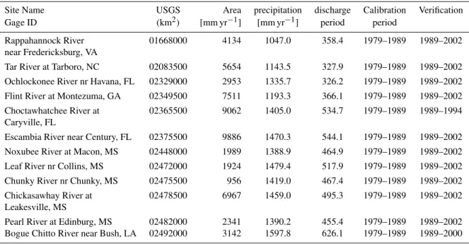
We undertake our verification assessment for 12 National Weather Service (NWS) forecast basins located in the South-eastern United States (Table 1). All basins fall within the Southeastern Plains ecoregion delineated by the Environ-mental Protection Agency (EPA) based on similar hydro-climatic characteristics, geomorphology, vegetation, and soil properties. The watersheds within this region have an array of vegetation types including cropland, pasture, woodland and forest. The streambeds in the southeastern plains have a low-gradient and sandy bottoms. The basins also gener-ally have no precipitation as snow. Data for each basin were collected from the Model Parameter Estimation eXperiment (MOPEX) database and spanned a period of 1 January 1948 to 30 September 2002. This region experiences a moderate climate with average temperature of 17.3◦C and average pre-cipitation of 1360 mm yr−1. The study watersheds range in size from less than 1000 km2to almost 10 000 km2(Table 1). 2.2 Modeling framework
Table 1. Study basins, basin area, and annual average precipitation and discharge for the period of record 1979–2002. Calibration and verification periods started 1 October and ended 30 September of the years indicated.
Site Name USGS Area precipitation discharge Calibration Verification
Gage ID (km2) [mm yr−1] [mm yr−1] period period
Rappahannock River 01668000 4134 1047.0 358.4 1979–1989 1989–2002
near Fredericksburg, VA
Tar River at Tarboro, NC 02083500 5654 1143.5 327.9 1979–1989 1989–2002
Ochlockonee River nr Havana, FL 02329000 2953 1335.7 326.2 1979–1989 1989–2002
Flint River at Montezuma, GA 02349500 7511 1193.3 366.1 1979–1989 1989–2002
Choctawhatchee River at 02365500 9062 1405.0 534.7 1979–1989 1989–1994
Caryville, FL
Escambia River near Century, FL 02375500 9886 1470.3 544.1 1979–1989 1989–2002
Noxubee River at Macon, MS 02448000 1989 1388.9 464.9 1979–1989 1989–2002
Leaf River nr Collins, MS 02472000 1924 1479.4 517.9 1979–1989 1989–2002
Chunky River nr Chunky, MS 02475500 956 1419.0 467.4 1979–1989 1989–2002
Chickasawhay River at 02478500 6967 1459.0 495.3 1979–1989 1989–2002
Leakesville, MS
Pearl River at Edinburg, MS 02482000 2341 1390.2 455.4 1979–1989 1989–2002
Bogue Chitto River near Bush, LA 02492000 3142 1597.8 626.1 1979–1989 1989–2000
account for water storage and flow through the subsurface. The upper layer represents surface soil regimes and inter-ception storage, while the lower layer represents deeper soil layers and groundwater storage (Brazil and Hudlow, 1981). Each layer consists of fast components (free water), driven mostly by gravitational forces, and slow components (ten-sion water), driven by evapotranspiration and diffu(ten-sion. The SAC-SMA is a saturation excess model; when precipitation amounts exceed percolation and interflow capacities, upper zone storage will overflow and overland flow will occur. Di-rect runoff also occurs from any impervious areas. There are 16 parameters in the SACSMA, of which 13 were calibrated (Table 2). Inputs to the model are basin-average precipita-tion and potential evapotranspiraprecipita-tion. The model output is channel inflow, which is routed to the basin outlet using a series of five linear reservoirs. The linear reservoir recession coefficient, K, was also optimized along with the 13 SAC-SMA parameters (Table 2). The SAC-SAC-SMA model was run at the daily time-step for each of the study basins. Calibra-tion was conducted using the ten year period 1 October 1979 to 30 September 1989. Model verification was conducted for the period of 1 October 1989–30 September 2002 (a shorter time period was used for the Choctawhatchee and Bogue Chitto Rivers based on the available record; Table 1). 2.3 Parameter identification methods
The Generalized Likelihood Uncertainty Estimator (GLUE) methodology is based on the concept that there is no one op-timal parameter set but many parameters sets that provide
relatively equal performance (Zak and Beven, 1999; Beven and Freer, 2001). In the GLUE methodology, feasible pa-rameter ranges must be specified from which many param-eter sets will be sampled. The model is run with each pa-rameter set and the output is evaluated against the observed variable of interest using a likelihood function to distinguish behavioral sets (accepted) and non-behavioral sets (rejected). The acceptability of the parameter set is based on a selected likelihood function meeting some threshold criteria which is subjectively pre-defined. The cumulative distribution of the likelihood function values is computed for the acceptable pa-rameter sets. To remove outliers, those sets with a likelihood function that falls within the middle 90% of the distribution are chosen.
In the current study, we apply GLUE by generating 10,000 parameter sets using Latin hypercube sampling (from a uni-form distribution). The SAC-SMA model is run for each of the 10 000 sets. We define behavioral parameters sets as any set that produce simulations with a pre-defined likelihood threshold, using a Nash-Sutcliffe Efficiency (NSE)>0.30 (Eq. 1, Sect. 2.4). This is a relatively non-restrictive thresh-old and the approach can result in a large number of behav-ioral sets.
Table 2.SACSMA model parameters and feasible range.
Parameter Description Units Range
UZTWM Upper-zone tension water maximum storage mm 1–150
UZFWM Upper-zone free water maximum storage mm 1–150
LZTWM Lower-zone tension water maximum storage mm 1–500
LZFPM Lower-zone free water primary maximum storage mm 1–1000
LZFSM Lower-zone free water supplementary storage mm 1–1000
UZK Upper-zone free water lateral depletion rate day−1 0.1–0.7
LZPK Lower-zone primary free water depletion rate day−1 0–0.2
LZSK Lower-zone supplementary free water depletion rate day−1 0.01–0.5
ADIMP Additional impervious area decimal fraction 0–0.4
PCTIM Impervious fraction of the watershed decimal fraction 0–0.1
ZPERC Maximum percolation rate dimensionless 1–249
REXP Exponent of the percolation equation dimensionless 0.5–4.5
PFREE Fraction of water percolating from upper zone directly decimal fraction 0–0.8 to lower-zone free water storage
K Five-level linear reservoir constant dimensionless 0.0–0.9
RIVA Riparian vegetation decimal fraction 0
SIDE Ratio of deep recharge to channel base flow decimal fraction 0.3 RSERV Fraction of lower-zone free water not transferable to decimal fraction 0
lower-zone tension water
computed using a Bayesian inference scheme (Box and Tiao, 1973). The population is then portioned into complexes, and a parallel sequence from each complex is initiated from the point (parameter set) that contains the highest posterior density. New candidate points are generated for each se-quence and a Metropolis-annealing criterion is used to eval-uate whether the new point should be added to the current sequence (Vrugt et al., 2006). If successful, new points will randomly replace existing members of the complex. After a prescribed number of iterations, new complexes are formed through shuffling. Evolution and shuffling are repeated until a targeted stationarity is reached in the Gelman-Rubin con-vergence diagnostic (Gelman and Rubin, 1992).
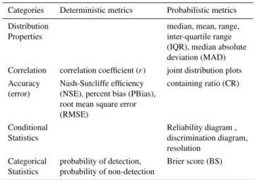
2.4 Verification methods
There are an extensive set of forecast verification measures that could be adopted for model evaluation. We selected those that are relevant to the modeling framework in the current study, are commonly applied, and have been iden-tified by the hydrologic forecast community as useful mea-sures. The Cooperative Program for Operational Meteorol-ogy, Education and Training (COMET®) Meteorology Ed-ucation and Training (MetEd) web-based module “Introduc-tion to Verifica“Introduc-tion of Hydrologic Forecasts” (for more infor-mation see http://www.meted.ucar.edu) and the NWS Hydro-logic Verification System Requirements Team report (NWS, 2006) describe seven forecast verification categories and list several deterministic and probabilistic metrics for each cat-egory. Our ensemble evaluation methodology is developed
Table 3.Statistical measures used for evaluation of parameter esti-mation methods and their respective categories.
Categories Deterministic metrics Probabilistic metrics
Distribution median, mean, range,
Properties inter-quartile range
(IQR), median absolute deviation (MAD) Correlation correlation coefficient (r) joint distribution plots Accuracy Nash-Sutcliffe efficiency containing ratio (CR) (error) (NSE), percent bias (PBias),
root mean square error (RMSE)
Conditional Reliability diagram ,
Statistics discrimination diagram,
resolution Categorical probability of detection, Brier score (BS) Statistics probability of non-detection
using five of the seven categories from these two sources (skill scores and confidence are not evaluated) and a sample of metrics from each category (Table 3). Metrics in the first category are used to assess the distribution properties of the ensembles. Metrics in categories two through five are used to evaluate the joint distribution of the simulations and obser-vations. The metrics were applied to the verification period only.
ensemble values and applying an empirical distribution. We first define{x(1),x(2),x(3),...x(z)}as the set of simulated
dis-charge values (the disdis-charge ensemble) sorted in ascending order for one timestep (t) from an ensemble of sizez. 2.4.1 Distribution properties
There are many measures of distribution, including the en-semble mean and median, but we are most interested in those that quantify the ensemble spread. Three metrics are used to evaluate the distribution of the ensemble members: the in-terquartile range (IQR), median absolute deviation (MAD), and range:
IQR = 1
n
n
X
t=1
(q0.75(t )−q0.25(t )) (1)
MAD = 1
n
n
X
t=1
mediani|xi(t )−xmed(t )| (2)
and Range = 1
n
n
X
t=1
x(1)(t )−x(z)(t )
(3) whereq0.75(t )andq0.25(t )are the 75th and 25th percentiles of the ensemble, respectively; xi(t )represents each
ensem-ble member for timestept;xmed(t )is the ensemble median;
x(1)(t )andx(z)(t )are the lowest and highest valued
ensem-ble members, respectively; andnis the number of timesteps (Wilks, 2006).
Equations (1)–(3) are also used to evaluate the parameter ensembles, in which case{x(1),x(2),x(3),...x(z)}is the set of
zvalues for a single model parameter normalized by the pa-rameter range (Table 2) andnbecomes the number of model parameters (14 in this study).
2.4.2 Correlation
The joint distribution of the observations and simulations is commonly evaluated through correlation measures or graphi-cally. In the deterministic approach, scatter plots and the cor-relation coefficient are used to assess the corcor-relation between the ensemble median and the observation. The correlation coefficient (r) is:
r=
n
N P t=1
(xmed(t )Qobs(t ))−
N P t=1
xmed(t )
·
N P t=1
Qobs(t )
s
n
N P t=1
xmed(t )2−
N P t=1
xmed(t )
2 · s n N P t=1
Qobs(t )2−
N P t=1
Qobs(t )
2
.(4)
whereQobs(t )is the observation at timet. In the probabilis-tic approach, the correlation between ensemble quantiles and the observations can be evaluated visually by plotting their joint distributions. Select ensemble quantiles (qk) are
cho-sen and plotted against the corresponding observation, where 0≤k≤1 (e.g.k= 0.10 (10th percentile),k= 0.25 (25th per-centile), etc.). This approach is similar to using a scatter plot.
2.4.3 Accuracy
The term accuracy refers to a measure of error in the sim-ulation ensemble when compared to the observation. Three common deterministic measures of model accuracy are used to assess the ensemble median: the Nash Sutcliffe efficiency score (NSE), root mean squared error (RMSE), and percent bias (Pbias):
NSE = 1 −
n
X
t=1
(xmed(t )−Qobs(t ))2/
n
X
t=1
Qobs(t )− Qobs(t )
2 ! , (5) RMSE = v u u t 1 n n X
t=1
(xmed(t )−Qobs(t ))2, (6)
Pbias =
n
X
t=1
(xmed(t )−Qobs(t ))
, n X
t=1
Qobs(t )
!
·100 %.(7)
A simple measure of ensemble accuracy is the Containing Ratio (CR) (Xiong and O’Connor, 2008):
CR = 1
n
n
X
t=1
I [Qobs(t )] (8)
whereI[·]is an indicator function as follows:
I[Qobs(t )] =
1, x(1)(t ) < Qobs(t ) < x(z)(t )
0,otherwise . (9)
I[Qobs(t )]equals 1 when the observation falls between the lowest and highest valued ensemble members andI[Qobs(t )] equals 0 when the observation falls outsize the ensemble bounds.
2.4.4 Conditional statistics
In the previous sections, we presented metrics that compare the simulated discharge values (i.e. median, minimum and maximum of the ensemble) to observed discharge values. In the following section, methods that evaluate probability values from the ensemble for specific discharge events are presented.
We first define mi(t ) as the probability of a simulated
streamflow event at a given timestep from the model ensem-ble, which can take on any ofI valuesm1(t ),m2(t)...mI(t )
(Wilks, 2006). The corresponding observation (yj(t )) can
take on any ofJ valuesy1(t ),y2(t )...yJ(t ). In this study,
The probability of a simulated streamflow event is derived by computing the percentage of the ensemble members that fall within each flow category at a given timestep. The proba-bility is rounded up to the nearest tenth probaproba-bility, therefore the probability will fall within one of ten possible probability bins (0–10 %,>10 %–20 %, etc.). At a given timestep, the observation will have a value of 1 (yj(t )= 1) for the flow
cat-egory in which it was observed, and a value of 0 (yj(t )= 0)
for the flow categories in which it did not occur.
Murphy and Winkler (1987) set up a general framework for forecast verification based on factorization of the joint distribution of forecasts and observations into the calibration-refinement factorization:
p mi, yj =p yj|mip(mi); i =1, ..., I; j =1, ..., J (10)
and the likelihood-base rate factorization: p mi, yj =p mi
yjp yj; i =1, ..., I; j =1, ..., J. (11)
The conditional distributionp(yj|mi) in Eq. (10) is the more
familiar measure of the two and can be plotted on a reliability diagram as a function of the ensemble probability. The en-semble probability is well calibrated if, for a given flow cat-egory, the relative frequency of the conditional event equals the ensemble probability (e.g.p(y= low flow|m= 0.1) =0.1) and when plotted on the reliability diagram, the conditional event will plot along a 1:1 line (Murphy and Winkler, 1987, 1992; Wilks, 2006). To avoid confusion with the model pa-rameter calibration discussion, hereafter we refer to the cali-bration of the ensemble probability as reliability.
The relative frequencies of the ensemble probabilities (p(mi)) are plotted as an inset on the reliability diagram
to indicate the sharpness, or resolution, of the ensembles (Wilks, 2006). Sharp ensembles will have narrowly dis-tributed probability values where probability occurs most fre-quently in the extreme probability categories (i.e. 0–10 % and
>90–100 %).
The likelihood distribution (p(mi|yj)) is a less intuitive
measure, but very useful for evaluating how much proba-bility the ensemble gives to the correct flow category com-pared to other possible categories. For all instances of an observation occurring in a given flow category, the condi-tional probability for all possible flows is computed: for ex-ample, the ensemble probability of a low flow given a low flow observation (p(m= low flow|y= low flow)), the ensem-ble probability of a middle flow given a low flow observation (p(m= middle flow|y= low flow)), and the ensemble proba-bility of a high flow given a low flow observation (p(m= high flow|y= low flow)). These likelihood distributions can then be plotted on the discrimination diagram as a function of the ensemble probability. Ensembles are highly accurate if the majority of the ensemble members frequently fall within the flow category observed (in the previous example, this would be the low flow category), resulting in high probabilities for the observed flow category and low probabilities for the re-maining flow categories. For such ensembles, the likelihood
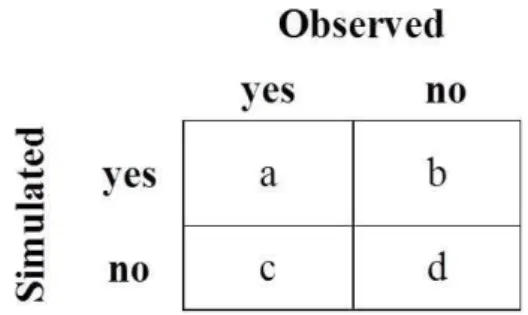
Fig. 1. Contingency table displaying the relationships between counts(a)–(d)of event pairs.
distributions for the different possible flows will not overlap to a great degree when plotted on the discrimination diagram and they are considered to have good discrimination for that flow category (Murphy and Winkler, 1987; Murphy et al., 1989; Wilks, 2006).
2.4.5 Categorical statistics
The categorical statistics listed in Table 3 are applicable to dichotomous events whereI=J= 2. These metrics are used here to evaluate the ability of the GLUE and SCEM ensem-bles to simulate floods. The magnitude of the flood dis-charge at the outlet gage for each watershed was obtained from the Lower Mississippi River Forecast Center website (http://www.srh.noaa.gov/lmrfc/).
The contingency table is a common method for verifying the joint distribution of non-probabilistic forecasts and ob-servations. This concept is applied to assess the ability of the ensemble median to identify flood (y(t )= 1) and no-flood (y(t )= 0) events. The model ensemble median is classified as flood (xmed(t )= 1) if its value is larger than flood stage and no-flood (xmed(t )= 0) if its value is smaller than flood stage. A 2×2 contingency table is set up (Fig. 1) and all possible observation/simulation pairs are counted. Two measures are used to summarize the contingency table (Wilks, 2006): the probability of detection (POD):
p(xmed(t ) = 1|y(t ) = 1) = POD =
a
a +c (12)
and the probability of false detection (POFD):
p(xmed(t ) = 1|y(t ) = 0) = POFD =
b
b +d. (13)
POD values equal to one and POFD values close to zero are optimum.
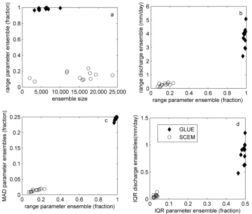
Fig. 2. Comparison of(a)parameter ensemble range to parameter ensemble size,(b)discharge ensemble range to parameter ensemble range,(c)mean absolute deviation (MAD) of the parameter ensembles to parameter ensemble range, and(d)interquartile range (IQR) of the discharge ensembles to IQR of the parameter ensembles for each study site. Parameters were normalized by their feasible range before computing the average parameter ranges, MADs and IQRs.
for flows higher than the flood level and the corresponding observations (y(t )) for all timesteps:
BS = 1
n
n
X
t=1
(mflood(t )−y(t ))2. (14)
A perfect BS is 0, and the score ranges from 0≤BS≤1 (Wilks, 2006).
3 Results
3.1 Distribution properties
Measures of distribution are first used to understand the na-ture of the parameter ensembles and their relation to the re-sulting discharge ensembles. In general we find weak pos-itive correlations between the measures compared (Fig. 2). Correlation between the parameter ensemble size and range (Fig. 2a) isr= 0.59 for the GLUE andr= 0.32 for the SCEM. Although the SCEM parameter ensembles are larger than the GLUE parameter ensembles, the range of the SCEM param-eter ensemble is much narrower, spanning less than 30 % of the feasible parameter space at all sites. The GLUE parame-ter values span almost the entire parameparame-ter space.
The range and IQR of the parameter and discharge en-sembles are compared in Fig. 2b and d, respectively. Both give similar information: the parameter ensembles that have values distributed across a larger portion of the parameter space produce discharge ensembles with a larger distribution of values. The IQR does reveal characteristics about the en-sembles that are not apparent when evaluating the range only. The IQRs of the SCEM parameter and discharge ensembles vary little among sites; by comparison the range values had more variation. This suggests that the central 50 % of the SCEM parameter sets are very similar, and the variation seen in the range comes from the upper and lower 25 % of the dis-tribution. Figure 2c indicates that as the parameter ensemble range increases, the values deviate more from the median, rather than being concentrated near the median with only a few outliers.
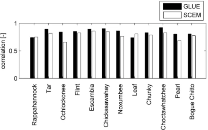
Fig. 3. The correlation coefficient for the ensemble median for all sites.
3.2 Correlation
On average, the ensemble medians from the GLUE and SCEM have good correlation to the discharge observations at the sites studied (Fig. 3). By plotting the joint distribution of the ensemble median and the observations it becomes ap-parent that the degree of correlation varies across the range of discharge values (Fig. 4, linexmed). In addition, the direction of the error (overestimating or underestimating the observa-tion) can vary across the range of discharge values. Results for the Leaf River (Fig. 4c and f) are similar to several sites studied (Chunky, Pearl, Bogue Chitto, Ochlocknee Rivers) in that the ensemble medians underestimate discharge at both the lower and upper end of the range of flows, but overesti-mate the middle range.
The 10th and 90th percentiles (q0.10 and q0.90,
respec-tively) of the GLUE ensembles almost always capture the low- and middle-range observations at all sites; whereas, the highest discharge ranges are often only contained within the upper 10 % (between q0.90 andqmax) (e.g. Fig. 4b and c). The SCEM ensembles (Fig. 4c–f) are narrow relative to the GLUE ensembles (Fig. 4a–c); this was also seen in Fig. 2b. In the Chickasawahay and the Noxumbee, the observation is mostly outside the bounds of the SCEM ensembles. The ability to capture the observation within the ensemble bounds will be quantified in the next section with the CR metric.
As was shown, plots of the joint distribution between the ensemble quantiles and the observation can be used to as-sess the performance of the median, the range of the ensem-ble and how well it captures the observation, and biases as a function of discharge magnitude. However, the informa-tion conveyed in Fig. 4 is potentially misleading. By de-picting the data as a line, it appears as though the frequency of the discharge values is equal across the entire range of flows. This is not the case. At the twelve sites studied, flows above 5 mm day−1represent only 2–6 % of the discharge ob-servations, and therefore the large biases seen in highest dis-charge values occur for a very small number of samples. An
alternative plotting scheme would be to plot the data as points rather than a line. However when 4745 points (the number of model timesteps) were plotted, the points overlapped each other at the lower discharge values (lower left corner of the plot) and the figure was difficult to read, particularly with the inclusion of multiple quantiles. In most modeling studies a long time period is preferred to assure sufficient calibration and verification of the model. However the large number of timesteps poses challenges from both the sampling stand-point (results are dominated by small discharge values which represent the majority of the samples used in computing the statistics) and the visualization standpoint.
3.3 Accuracy
The NSE, RMSE, and Pbias are common measures of model accuracy and are used to evaluate the ensemble median (Fig. 5). While useful for giving a concise assessment of model skill, the skill of the ensemble median for dif-ferent magnitudes of discharge obviously cannot be under-stood from these numbers. In Fig. 4 we observed that the GLUE ensemble median tends to overestimate flows less than 5 mm day−1and underestimate flows above that level. The SCEM ensemble medians on the other hand have a ten-dency to overestimate all flow ranges. As a result, the Pbias (Fig. 5b) and RMSE (Fig. 5c) of the GLUE are smaller than the SCEM, but for high flows neither method tends to be most accurate. Metrics in Fig. 5 measure summarize performance of the ensemble median for all timesteps, therefore, their value will be dominated by the skill of the ensemble median for low flow events. The large number of small discharge ob-servations was also mentioned in the previous section and is a significant limitation of traditional model evaluation meth-ods given that many hydrologic model applications are fo-cused on simulating and predicting very high flows.
The advantage to using the measures in Figs. 3 and 5 is that most people in the hydrologic modeling community are familiar with them. However, comparison of results between different modeling studies is difficult because the accuracy of the model simulations are influenced by data quality and the hydrologic characteristics of the time period studied, which may vary from one study to the next. Additionally, the value of the RMSE scores is a function of the discharge magnitude for the study site. In this study, comparison of the two pa-rameter estimation methods is only possible because we are applying both methods with the same model, time period, and study sites.
Fig. 4. The joint distribution of the lowest (qmin), highest (qmax), 10th (q0.1), and 90th (q0.9) percentiles, and the median (xmed, or 50th percentile) of the discharge ensembles and the observations from the(a)–(c)GLUE and(d)–(f)SCEM parameter estimation methods for select sites. The solid black line in the figures is the 1:1 line and indicates perfect correlation between the simulated and observed discharge.
timestep. Therefore they may not be applicable to this study which uses a daily timestep.
The CR is used to assess the accuracy of the ensemble bounds rather than focusing only on the median (Fig. 6). Given the biases and narrow range of the SCEM ensembles observed in Fig. 4, it is not surprising that the CR values are lower for this parameter estimation method. GLUE, which has much wider bounds captures the observations at a higher rate. Thus, CR is positively correlated with the range of the discharge and parameter ensembles for these parameter esti-mation methods (Fig. 6a and b). We also compute the CR by category by separating ensembles into one of three flow cat-egories based on which observation occurred (low, middle, or high flow). The CR for each method are fairly consistent across all flow ranges but are slightly better for low flows (Fig. 6c).
In its standard application, the CR provides a useful sum-mary of the accuracy of the uncertainty bounds, but does not consider the distribution of the ensemble members. It also cannot reveal whether the ensemble is over- or under-estimating the observation. More detailed information about the ensemble member distributions and associated perfor-mance can be obtained by considering multiple intervals within the ensemble, rather than the ensemble bounds only such as through the application of the rank histogram (Hamill and Collucci, 1997; Hamill, 2001; Wilks, 2006) or spread-bias diagram (Brown et al., 2010).
At a minimum, containing the observation within the un-certainty bounds is desired. However, an ensemble in which most members fall near the observation (indicating high probability for that observation) is more useful than an en-semble in which the members are equally distributed across many possible flow values (indicating similar probability for many possible observations). The conditional statistics in the next section are used to evaluate the probability distribution of the ensemble.
3.4 Conditional statistics
Fig. 5. The(a)Nash Sutcliffe Efficiency (NSE),(b)percent bias (Pbias), and(c)root mean square error (RMSE) for the ensemble median for all sites.
for high probabilities by the SCEM ensembles at many sites (Fig. 7d–f).
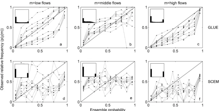
Classic calibration and verification approaches evaluate the simulation on the basis of how well the simulation matches the observation at each timestep. The reliability di-agrams indicate that this practice does not assure that the en-semble probabilities will reflect the frequency of the observa-tions. However, because the number of samples in the mid-dle probability bins is so small, particularly for the SCEM (Fig. 7d–f, insets), interpretation of the reliability results for those bins is difficult. The poor reliability results for ensem-ble probabilities between 20 % and 80 % (Fig. 7d–f) may be because there are too few samples to provide a good assess-ment of the ensemble.
The high frequency of ensemble probabilities within the 0–10 % and 90–100 % probability bins for the SCEM (Fig. 7d–f, inset) indicate high refinement or resolution. The GLUE ensembles are comparably less refined with more instances of ensemble probability in the 20–80 % range (Fig. 7a–c, inset). The small range of the SCEM ensem-bles (Fig. 2a and b) led to higher refinement of the ensemble probabilities.
For illustration purposes, results from the discrimination analysis have been averaged together for all sites for each parameter estimation methods (Fig. 8); for analysis of an in-dividual site, one figure like Fig. 8 would be needed for each site. All methods produce ensembles with good discrimina-tion for low flows (Fig. 8a and d) and high flows (Fig. 8c and f), and poorer discrimination for middle flows (Fig. 8b and e). When either a high or low flow occurs, the ensem-bles have the most difficulty discriminating the probability of the observed flow from the probability of middle flows. But they are skillful in not giving large probability to the extreme opposite category.
The low range of the SCEM (Fig. 2a and b) led to bet-ter discrimination of flows in all flow categories compared to the GLUE because the probabilities of the SCEM ensembles were better resolved (more probabilities in the extreme prob-ability bins). However, the narrow range of the SCEM en-semble led to poorer performances in metrics that evaluated the ability of the ensemble to capture the event within the uncertainty bounds (i.e. the CR, Fig. 6). The higher ensem-ble spread in the GLUE (Fig. 2a and b) led to ensemensem-bles that tended to distribute the probability among the possible flow categories. For example, GLUE ensembles frequently as-signed probability to low and high flows when middle flows occur, resulting in relatively poor discrimination for middle flows (Fig. 8b). Therefore, while the CR is high for the GLUE, the discrimination is lower compared to the SCEM.
Unlike some of the other methods presented here, reliabil-ity and discrimination are easy to interpret for an individual parameter estimation method or site without the need to com-pare to another example. The use of flow categories in this section allows for assessment of model performance under different conditions (i.e. low flows versus high flows) pro-viding more information than the summary measures can. However, the choice of flow levels based on climatological thresholds introduces a somewhat arbitrary cut off point for analysis. While the use of reliability does not require the use of flow categories, metrics such as discrimination require some degree of categorization. Additionally, we chose to use probability intervals of 10 %, another subjective decision that can be adjusted to varying situations and needs.
3.5 Categorical statistics
In the final analysis, three metrics are used to evaluate the simulation of flood events. No flood level was available for the Rappahannock River, and therefore this site was not used in the analysis. At least one flood was observed during the evaluation period at all sites.
Fig. 6. Comparison of the containing ratios (CR) to the(a)discharge ensemble ranges and(b)parameter ensemble ranges; and(c)the average CR from the study sites by flow category (low, middle, high).
Fig. 8. Discrimination diagrams for simulation ensembles when the observations were in the(a,d)low,(b,e)middle, and(c,f)high flow categories from the(a)–(c)GLUE and(d)–(f)SCEM methods. The diagram depicts the average of results from all sites.
methods perform similarly. Recall from Fig. 4 that the me-dians tend to underestimate the highest flows, this negative bias in the upper range of the discharge values results in low POFD scores (Fig. 9b). The large negative bias in the median for the Leaf (Fig. 4c and f) and Chunky Rivers (not shown in Fig. 4) leads to a low POFD (Fig. 9b), but results in no skill for POD (Fig. 9a) at these sites.
The BS is used to evaluate the ensemble probability for a flood event (Fig. 10a). While the perfect BS is zero, this is another metric for which the number itself holds little mean-ing without comparison to other ensembles. When evaluat-ing forecasts, the BS from the forecasts are often compared to climatology. In our comparison, the GLUE has slightly bet-ter BSs than the SCEM because the range of the ensembles is larger and, therefore, the ensemble tend to assign some prob-ability to flood events when they occur. Comparing these re-sults to the frequency at which floods are simulated by each model (Fig. 10b), it is apparent that the SCEM ensembles give 0 % chance of flows above flood stage on average 95 % of the time. The GLUE gives probability for floods more fre-quently. As a result, the SCEM does more poorly than the GLUE for the BS.
Note that the BS for predictions above flood stage pro-duce the same BS for predictions below flood stage. For this reason, the failure for the ensemble to simulate floods for Leaf and Chunky Rivers (Fig. 9a), produces a very low BS (Fig. 10a) because they predict no-floods well. Because this summary value is an evaluation of no-flood as well as flood events, it is heavily influenced by the large number of
timesteps with no-flood. This leads to very low BSs event though the ensembles tended to have larger biases for very high flows.
4 Concluding remarks
When evaluating ensembles of simulations, deterministic metrics are often applied to the median or expected value. This practice ultimately removes a significant amount of en-semble information from the evaluation process. We have demonstrated a sampling of metrics that are traditionally applied for verification of forecasts, and have shown these to be informative for evaluation and comparison of ensem-ble streamflow simulations. A consideraensem-ble amount of in-formation about the uncertainty estimation methods can be obtained when treating the simulations in a probabilistic manner.
Fig. 9.The(a)probability of detection for floods and(b)probability of non-detection for floods for the ensemble medians at each site.
categories and the joint distribution plots allow analysis of the ensembles for discharge levels of interest.
We have identified some challenges when using forecast verification metrics for model ensemble evaluation. First, most forecast verification metrics were developed for fore-casts of a single variable (e.g. rain or no rain, or peak dis-charge) to occur over some forecast interval, whereas model simulations produce a continuous variable most often eval-uated at the model timestep. This means that in the case of evaluating model simulations, the sample size will likely be very large. Furthermore, the number of timesteps with low flows will be very large relative to the higher flows and model skill for low flows will dominate the results. Because low flows are often the range of least interest, approaches to limit the influence of low discharge events on the statistics should be investigated. One possible approach to deal with varia-tions in sample sizes across flow regimes is to evaluate cat-egories of flows as shown. But careful consideration of the influence of the sample size and sampling distribution on the confidence of the verification metric, an issue not addressed in this study, should be taken (Bradley et al., 2003; Wilks, 2006). Because probabilistic statistics rely on a significant number of model-observation pairs to obtain meaningful re-sults (Wilks, 2006), evaluation of the model uncertainty asso-ciated with flood events will be limited by small sample sizes in most cases. Common problems such as identifying flow and probability thresholds or appropriate distributions exist and, because they may be treated differently in different stud-ies, will limit the ability to compare results across different studies. Finally, we did not test for time-dependent cluster-ing of the ensemble members or independence of the events analyzed, such as described by Christoffersen (1998), to de-termine statistical correctness. There is significant memory in a sequence of hydrologic model outputs and hydrologic
Fig. 10.The(a)Brier score for simulations of flood events for each site, and(b)cumulative frequency of the ensemble probability for flow above flood stage.
observations, which violates the assumption of sample inde-pendence. Investigation of this issue with respect to hydro-logic model and forecast verification is a recommended topic for future studies.
Nonetheless, advanced probabilistic verification metrics developed for forecast verification provide a rigorous plat-form by which modeling methods can be evaluated and com-pared. The application of these metrics requires no infor-mation in addition to what is already available as part of the traditional model validation methodology, and allows con-sideration of the entire ensemble or uncertainty range in the approach. These measures are much more informative about the nature of model uncertainty estimates than simple deter-ministic measures. Through our efforts in this and future papers, we hope to advance discussion about evaluation of simulation uncertainty and more robust model verification measures.
Acknowledgements. We would like to thank James Brown and two anonymous reviewers for their helpful comments on an earlier draft of this paper. We would also like to thank Alexandre Dulac and Sonya Lopez for their contributions to this work. This research was partially supported by a grant from the National Oceanic Atmospheric Administration (NOAA) National Weather Service (#NA07NWS4620013) and the National Aeronautics and Space Administration (#NNX10AQ77G).
References
Ajami, N. K., Duan, Q., and Sorooshian, S.: An integrated hy-drologic Bayesian multimodel combination framework: Con-fronting input, parameter, and model structural uncertainty in hydrologic prediction, Water Resour. Res., 43, W01403, doi:10.1029/2005WR004745, 2007.
Bartholmes, J. C., Thielen, J., Ramos, M. H., and Gentilini, S.: The european flood alert system EFAS – Part 2: Statistical skill as-sessment of probabilistic and deterministic operational forecasts, Hydrol. Earth Syst. Sci., 13, 141–153, doi:10.5194/hess-13-141-2009, 2009.
Beven, K.: A manifesto for the equifinality thesis, J. Hydrol., 320, 18–36, 2006.
Beven, K. and Binley, A.: Future of distributed models: Model cali-bration and uncertainty prediction, Hydrol. Process., 6, 279–298, 1992.
Beven, K. and Freer, J.: Equifinality, data assimilation, and uncer-tainty estimation in mechanistic modelling of complex environ-mental systems using the GLUE methodology, J. Hydrol., 249, 11–29, doi:10.1016/S0022-1694(01)00421-8, 2001.
Box, G. E. P. and Tiao, G. C.: Bayesian Inference in Statistical Analysis, Addison-Wesley, 1973.
Bradley, A. A. and Schwartz, S. S.: Summary verification measures and their interpretation for ensemble forecasts, Mon. Weather Rev., 3075–3089, 2011.
Bradley, A. A., Hashino, T., and Schwartz, S. S.: Distributions-oriented verification of probability forecast for small data sam-ples, Weather Forecast., 18, 903–917, 2003.
Bradley, A. A., Schwartz, S. S., and Hashino, T.: Distributions-oriented verification of ensemble streamflow predictions, J. Hy-drometeorol., 5, 532–545, 2004.
Brazil, L. E. and Hudlow, M. D.: Calibration procedures used with the National Weather Service Forecast System, in: Water and Realted Land Resource Systems, edited by: Haimes, Y. Y. and Kindler, J., Pergamon, Tarrytown, N.Y., 457–466, 1981. Brier, G. W.: Verification of forecasts expressed in terms of
proba-bilities, Mon. Weather Rev., 78, 1–3, 1950.
Brown, J., Demargne, J., Seo, D.-J., and Liu, Y.: The Ensem-ble Verification System (EVS): a software tool for verifying en-semble forecasts of hydrometeorological and hydrologic vari-ables at discrete locations, Environ. Modell. Softw., 25, 854–872, doi:10/1016/j.envsoft.2010.01.009, 2010.
Burnash, R. J., Ferral, R. L., and McGuire, R. A.: A Generalized Streamflow Simulation System Conceptual: Modeling for Digi-tal Computers, Joint Federal-State River Forecast Center, Sacra-mento, CA, 1973.
Clark, M. P. and Kavetski, D.: Ancient numerical daemons of conceptual hydrological modeling: 1. Fidelity and efficiency of time stepping schemes, Water Resour. Res., 46, W10510, doi:10.1029/2009WR008894, 2010.
Coccia, G. and Todini, E.: Recent developments in predictive uncertainty assessment based on the model conditional pro-cessor approach, Hydrol. Earth Syst. Sci., 15, 3253–3274, doi:10.5194/hess-15-3253-2011, 2011.
Cooke, W. E.: Forecasts and verifications in Western Australia, Mon. Weather Rev., 34, 23–24, 1906.
Christoffersen, P. F.: Evaluating interval forecasts, Int. Econ. Rev., 39, 841–862, 1998.
Day, G. N.: Extended streamflow forecasting using NWSRFS, J. Water Resour. Plann. Manage., 111, 157–170, 1985.
De Finetti, B.: Foresight: its logical laws, its subjective sources, in: Studies in Subjective Probability, edited y: Kyburg Jr., H. E. and Smokler, H. E., Wiley, New York, 1964, 94–158, 1937. De Lannoy, G. J. M., Houser, P. R., Pauwels, V. R. N., and Verhoest,
N. E. C.: Assessment of model uncertainty for soil moisture through ensemble verification, J. Geophys. Res., 111, D10101, doi:10.1029/2005JD006367, 2006.
Demargne, J., Brown, J., Liu, Y., Seo, D. J., Wu, L., Toth, Z., and Zhu, Y.: Diagnostic verification of hydrometerological ensem-bles, Atmos. Sci. Lett., 11, 114–122, 2010.
Duan, Q., Sorooshian, S., and Gupta, V.: Effective and efficient global optimization for conceptual rainfall-runoff models, Water Resour. Res., 28, 1015–1031, 1992.
Duan, Q., Gupta, V. K., and Sorooshian, S.: A Shuffled Complex Evolution Approach for Effective and Efficient Global Optimiza-tion, J. Opt. Theory App., 76, 501–521, 1993.
Duan, Q., Ajami, N. K., Gao, X., and Sorooshian, S.: Multi-model ensemble hydrologic prediction using Bayesian model averag-ing, Adv. Water Resour., 30, 1371–1386, 2007.
Evensen, G.: Sequential data assimilation with a nonlinear quasi-geostrophic model using Monte Carlo methods to forecast error statistics, J. Geophys. Res., 99, 10143–10162, 1994.
Faber, B. A. and Stedinger, J. R.: Reservoir optimization using sam-pling SDP with ensemble streamflow prediction (ESP) forecasts, J. Hydrol., 249, 113–133, 2001.
Finley, J. P.: Tornado predictions, Am. Meteorol. J., 1, 85–88, 1884. Franz, K. J., Hartmann, H. C., Sorooshian, S., and Bales, R.: Veri-fication of National Weather Service Ensemble Streamflow Pre-dictions for water supply forecasting in the Colorado River basin, J. Hydrometeorol., 4, 1105–1118, 2003.
Franz, K. J., Hogue, T., and Sorooshian, S.: Snow model verifica-tion using ensemble predicverifica-tion and operaverifica-tional benchmarks, J. Hydrometeorol., 9, 1402–1415, 2008.
Franz, K. J., Butcher, P., and Ajami, N. K.: Addressing snow model uncertainty for hydrologic prediction, Adv. Water Resour., 33, 820–832, 2010.
Gelman, A. And Rubin, D. B.: Inference from iterative simulation using multiple sequences, Stat. Sci., 7, 457–472, 1992.
Gupta, H. V., Beven, K. J., and Wagener, T.: Model calibration and uncertainty estimation, in: Encyclopedia of Hydrologic Sci-ences, edited by: Anderson, M. G. and Mcconnell, J. J., John Wiley, New York, 2015–2031, 2006.
Hamill, T. M.: Interpretation of the rank histogram for verifying ensemble forecasts, Mon. Weather Rev., 129, 550–560, 2001. Hamill, T. M. and Collucci, S. J.: Verification of Eta-RSM
short-range ensemble forecasts, Mon. Weather Rev., 125, 1312–1327, 1997.
Hastings, W. K.: Monte-Carlo sampling methods using Markov Chains and their applications, Biometrika, 57, 97–109, 1970. Jolliffe, I. T. and Stephenson, D. B.: Forecast Verification: A
Prac-tioner’s Guide in Atmospheric Science, John Wiley and Sons, Chichester, 240 pp., 2003.
Kitanidis, P. K. and Bras, R. L.: Real-time forecasting with a con-ceptual hydrologic model I. analysis of uncertainty, Water Re-sour. Res., 16, 1025–1033, 1980a.
Kitanidis, P. K. and Bras, R. L.: Real-Time Forecasting with a con-ceptual hydrologic model 2. applications and results, Water Re-sour. Res., 16, 1034–1044, 1980b.
Krzysztofowicz, R.: The case for probabilistic forecasting in hy-drology, J. Hydrol., 249, 2–9, 2001.
Krzysztofowicz, R. and Kelly, K. S.: Hydrologic uncertainty pro-cessor for probabilistic river stage forecasting, Water Resour. Res., 36, 3265–3277, 2000.
Laio, F. and Tamea, S.: Verification tools for probabilistic forecasts of continuous hydrological variables, Hydrol. Earth Syst. Sci., 11, 1267–1277, doi:10.5194/hess-11-1267-2007, 2007. Margulis, S. A., McLaughlin, D., Entekhabi, D., and Dunne,
S.: Land data assimilation and estimation of soil mois-ture using measurements from the Southern Great Plains 1997 Field Experiment, Water Resour. Res., 38, 1299, doi:10.1029/2001WR001114, 2002.
Mason, S. J. and Graham, N. E.: Conditional probabilities, relative operating characteristics, and relative operating levels, Weather Forecast., 14, 713–725, 1999.
Metropolis, N., Rosenbluth, A. W., Rosenbluth, M. N., Teller, A. H., and Teller, E.: Equations of state calculations by fast computing machines, J. Chem. Phys., 21, 1087–1091, 1953.
Montanari, A. and Brath, A.: A stochastic approach for assess-ing the uncertainty of rainfall-runoff simulations, Water Resour. Res., 40, W01106, doi:10.1029/2003WR002540, 2004. Moriasi, D. N., Arnold, J. G., Van Liew, M. W., Bingner, R. L.,
Harmel, R. D., and Veith, T. L.: Model evaluation guidelines for systematic quantification of accuracy in watershed simulations, Trans, ASABE, 50, 885–900, 2007.
Muleta, M. K. and Nicklow, J. W.: Sensitivity and uncertainty anal-ysis coupled with automatic calibration for a distributed water-shed model, J. Hydrol., 306, 127–145, 2005.
Murphy, A. H.: A note on the utility of probabilistic predictions and the probability score in the cost–loss ratio decision situation, J. Appl. Meteorol., 5, 534–537, 1966.
Murphy, A. H.: Forecast verification: Its complexity and dimen-sionality, Mon. Weather Rev., 119, 1590–1601, 1991.
Murphy, A. H.: A coherent method of stratification within a gen-eral framework for forecast verification, Mon. Weather Rev., 123, 1582–1588, 1995.
Murphy, A. H.: The Finley affair: A signal event in the history of forecast verification, Weather Forecast., 11, 3–20, 1996. Murphy, A. H.: Forecast Verification, in: Economic value of
weather and climate forecasts, edited by: Katz, R. W. and Murphy, A. H., Cambridge University Press, Cambridge, MA, 240 pp., 1997.
Murphy, A. H. and Epstein, E. S.: A note on probability forecasts and “Hedging”, J. Appl. Meteorol., 6, 1002–1004, 1967. Murphy, A. H. and Wilks, D. S.: A case study of the use of
sta-tistical models in forecast verification: Precipitation probability forecasts, Weather Forecast., 13, 795–810, 1998.
Murphy, A. H. and Winkler, R. L.: A general framework for forecast verification, Mon. Weather Rev., 115, 1330–1338, 1987. Murphy, A. H. and Winkler, R. L.: Diagnostic verification of
prob-ability forecasts, Hydrol. Process., 7, 435–455, 1992.
Murphey, A. H., Brown, B. G., and Chen, Y.: Diagnostic verifi-cation of temperature forecasts, Weather Forecast., 4, 485–501, 1989.
NWS: National Weather Service River Forecast Verification Plan, Report of the Hydrologic Verification System Requirements Team, October 2006, http://nws.noaa.gov/oh/rfcdev/docs/Final Verification Report.pdf, last access: October 2010, US Depart-ment of Commerce, NOAA/NWS, Silver Spring, Maryland, 2006.
Ramsey, F. P.: Truth and Probability, in: The Foundations of Math-ematics and Other Logical Essays, edited by: Braithwaite, R. B.,Humanities Press, New York, 1950, 156–198, 1926.
Randrianasolo, A., Ramos, M. H., Thirel, G., Andr´eassian, V., and Martin, E.: Comparing the Scores of hydrologic ensemble fore-casts issued by two different hydrological models, Atmos. Sci. Lett., 11, 100–107, 2010.
Renner, M., Werner, M. G. F., Rademacher, S., and Sprokkereef, E.: Verification of ensemble flow forecasts for the River Rhine, J. Hydrol., 376, 463–475, doi:10.1016/j.jhydrol.2009.07.059, 2009.
Schoups, G., Vrugt, J. A., Fenicia, F., and van de Giesen, N. C.: Corruption of accuracy and efficiency of Markov chain Monte Carlo simulation by inaccurate numerical implementation of conceptual hydrologic models, Water Resour. Res., 46, W10530, doi:10.1029/2009WR008648, 2010.
Seo, D. J., Koren, V., and Cajina, N.: Real-time variational assimila-tion of hydrologic and hydrometeorological data into operaassimila-tional hydrologic forecasting, J. Hydrometeorol., 4, 627–641, 2003. Seo, D. J., Cajina, L., Corby, R., and Howieson, T.: Automatic state
updating for operational streamflow forecasting via variational data assimilation, J. Hydrol., 367, 255–275, 2009.
Shrestha, D. L., Kayastha, N., and Solomatine, D. P.: A novel ap-proach to parameter uncertainty analysis of hydrological models using neural networks, Hydrol. Earth Syst. Sci., 13, 1235–1248, doi:10.5194/hess-13-1235-2009, 2009.
Thirel, G., Rousset-Regimbeau, F., Martin, E., and Habets, F.: On the impact of short-range meteorological forecasts for Ensemble Streamflow Predictions, J. Hydrometeorol., 9, 1301–1317, 2008. Verbunt, M., Zappa, M., Gurtz, J., and Kaufmann, P.: Verifica-tion of a coupled hydrometeorological modeling approach for alpine tributaries in the Rhine basin, J. Hydrol., 324, 224–238, doi:10.1016/j.jhydrol.2005.09.036, 2006.
Vrugt, J. A. and Robinson, B. A.: Treatment of uncertainty using ensemble methods: Comparison of sequential data assimilation and Bayesian model averaging, Water Resour. Res., 43, W01411, doi:10.1029/2005WR004838, 2007.
Vrugt, J. A., Gupta, H. V., Bouten, W., and Sorooshian, S.: A shuffled complex evolution Metropolis algorithm for optimiza-tion and uncertainty assessment of hydrological model parame-ters, Water Resour. Res., 39, 1201, 2003.
Vrugt, J. A., Gupta, H. V., Nuallain, B., and Bouten, W.: Real-time data assimilation for operational ensemble streamflow forecast-ing, J. Hydrometeorol., 7, 548–565, 2006.
Wilks, D. S.: Resampling hypothesis tests for autocorrelated fields, J. Climate, 10, 65–82, 1997.
Wilks, D. S.: Multisite generalizations of a daily stochastic precip-itation generation model, J. Hydrol., 210, 178–191, 1998. Wilks, D. S.: Statistical Methods in the Atmospheric Sciences,
2nd Edn., Academic Press, Amsterdam, 627 pp., 2006.
Xiong, L. and O’Connor, K. M.: An empirical method to improve the prediction limits of the GLUE methodology in rainfall-runoff modeling, J. Hydrol., 349, 115–124, 2008.