www.atmos-chem-phys.net/17/1673/2017/ doi:10.5194/acp-17-1673-2017
© Author(s) 2017. CC Attribution 3.0 License.
Impact of biogenic very short-lived bromine on the Antarctic ozone
hole during the 21st century
Rafael P. Fernandez1,2, Douglas E. Kinnison3, Jean-Francois Lamarque3, Simone Tilmes3, and Alfonso Saiz-Lopez1
1Department of Atmospheric Chemistry and Climate, Institute of Physical Chemistry Rocasolano,
CSIC, Madrid, 28006, Spain
2National Research Council (CONICET), FCEN-UNCuyo, UNT-FRM, Mendoza, 5500, Argentina
3Atmospheric Chemistry, Observations & Modelling Laboratory, National Center for Atmospheric Research,
Boulder, CO 80301, USA
Correspondence to:Alfonso Saiz-Lopez (a.saiz@csic.es)
Received: 21 September 2016 – Published in Atmos. Chem. Phys. Discuss.: 5 October 2016 Revised: 26 December 2016 – Accepted: 9 January 2017 – Published: 3 February 2017
Abstract. Active bromine released from the photochemical decomposition of biogenic very short-lived bromocarbons (VSLBr)enhances stratospheric ozone depletion. Based on a dual set of 1960–2100 coupled chemistry–climate simula-tions (i.e. with and without VSLBr), we show that the maxi-mum Antarctic ozone hole depletion increases by up to 14 % when natural VSLBrare considered, which is in better
agree-ment with ozone observations. The impact of the additional 5 pptv VSLBr on Antarctic ozone is most evident in the pe-riphery of the ozone hole, producing an expansion of the ozone hole area of ∼5 million km2, which is equivalent in magnitude to the recently estimated Antarctic ozone heal-ing due to the implementation of the Montreal Protocol. We find that the inclusion of VSLBr in CAM-Chem (Commu-nity Atmosphere Model with Chemistry, version 4.0) does not introduce a significant delay of the modelled ozone re-turn date to 1980 October levels, but instead affects the depth and duration of the simulated ozone hole. Our analysis fur-ther shows that total bromine-catalysed ozone destruction in the lower stratosphere surpasses that of chlorine by the year 2070 and indicates that natural VSLBrchemistry would dom-inate Antarctic ozone seasonality before the end of the 21st century. This work suggests a large influence of biogenic bromine on the future Antarctic ozone layer.
1 Introduction
The detection of the springtime Antarctic ozone hole (Far-man et al., 1985) has been one of the great geophysical dis-coveries of the 20th century. The unambiguous scientific re-ports describing the active role of halogen atoms (i.e. chlo-rine and bromine), released from anthropogenic chloroflu-orocarbons (CFCs) and halons, in depleting stratospheric ozone (Molina and Rowland, 1974; McElroy et al., 1986; Daniel et al., 1999) led to the rapid and efficient implemen-tation of the Montreal Protocol in 1989 (Solomon, 1999). Since then, the consequent turnover on the anthropogenic emissions of long-lived chlorine (LLCl)and bromine (LLBr)
sources (WMO, 2014) has controlled the evolution of the strong springtime ozone depletion within the Antarctic vor-tex, and the first signs of recovery of the ozone hole became evident at the beginning of the 21st century (WMO, 2014; Chipperfield et al., 2015; Solomon et al., 2016).
pogenic emissions, an additional contribution from biogenic very short-lived bromocarbons (VSLBr). This additional
in-put of bromine is required to reconcile current stratospheric bromine trends (Salawitch et al., 2010; WMO, 2014).
VSLBrare naturally released from biologically productive waters mainly within the tropical oceans (Warwick et al., 2006; Butler et al., 2007; Kerkweg et al., 2008), where strong convective uplifts efficiently entrain near surface air into the upper troposphere and lower stratosphere (Aschmann and Sinnhuber, 2013; Liang et al., 2014; Saiz-Lopez and Fernan-dez, 2016). The current contribution of VSLBrto total strato-spheric inorganic bromine is estimated to be in the range of 3–8 pptv (Montzka et al., 2011; WMO, 2014; Navarro et al., 2015; Hossaini et al., 2016). The most accepted value for stratospheric injection is VSLBr≈5 pptv, which currently represents approximately 30 % of the total contribution from LLBr substances arising from both anthropogenic and nat-ural origins (∼7.8 pptv Halons+ ∼7.2 pptv CH3Br≈15–
16 pptv LLBr). The additional stratospheric contribution of biogenic VSLBrimproves the model–observation agreement with respect to stratospheric ozone trends between 1980 and the present (Sinnhuber et al., 2009), with large ozone-depleting impacts during periods of high aerosol loading within mid-latitudes (Feng et al., 2007; Sinnhuber and Meul, 2015). Although we still lack a scientific consensus with respect to the future evolution of VSLBr oceanic source strength and stratospheric injection (WMO, 2014), it will probably increase in the future following the increase in sea surface temperature (SST) and oceanic nutrient supply, as well as due to the enhancement of the troposphere-to-stratosphere exchange (Hossaini et al., 2012; Leedham et al., 2013).
Previous chemistry-climate modelling studies considering VSLBrchemistry mainly focused on improving the model vs. observed ozone trends at mid-latitudes with respect to equiv-alent set-ups considering only the dominant anthropogenic LLCl and LLBr sources (Feng et al., 2007; Sinnhuber et al., 2009). However, those previous studies lack an in-depth timeline analysis of the VSLBr impact on the ozone hole evolution during the current century. More recently, Sinnhu-ber and Meul (2015) found that the impact of VSLBr max-imises the Antarctic ozone hole (∼20 % greater ozone
de-coupled (with an interactive ocean) chemistry-climate sim-ulations from 1960 to 2100 with and without the contribu-tion of oceanic VSLBrsources. We focus on natural VSLBr -driven changes in the chemical composition and evolution of the Antarctic ozone hole during the 21st century, partic-ularly on their influence on the seasonality and enlargement of the ozone hole area, ozone hole depth and return date to 1980 levels. The analysis shown here describes the ozone hole progress distinguishing the monthly seasonality from the long-term evolution. Additionally, we present a timeline assessment of individual contribution of anthropogenic and natural chlorine and bromine species to Antarctic ozone loss during the 21st century, recognising the independent impact arising from LLBrand VSLBrsources to the overall halogen-catalysed O3destruction.
2 Methods
The three-dimensional chemistry climate model CAM-Chem (Community Atmospheric Model with Chemistry, version 4.0)(Lamarque et al., 2012), included in the CESM frame-work (Community Earth System Model, version 1.1.1) has been used for this study. The model set-up is identical to the CCMI-REFC2 experiment described in detail by Tilmes et al. (2016), with the exception that the current configu-ration includes a full halogen chemistry mechanism from the earth surface to the lower stratosphere (Fernandez et al., 2014), i.e. instead of considering a constant lower bound-ary condition of 1.2 pptv for bromoform (CHBr3) and
di-bromomethane (CH2Br2) or increasing CH3Br by 5 pptv,
our model set-up includes geographically distributed and seasonal-dependent oceanic emissions of six bromocarbons (VSLBr=CHBr3, CH2Br2, CH2BrCl, CHBrCl2, CHBr2Cl
and CH2IBr) (Ordóñez et al., 2012). At the model surface
moder-ate Representation Concentration Pathway 6.0 (RCP6.0) sce-nario (see Eyring et al., 2013, for a complete description of REFC2-CCMI set-up). In order to avoid unnecessary uncer-tainties associated with the speculative evolution of VSLBr oceanic emissions, we used a constant annual source strength for the whole modelled period.
CAM-Chem was configured with a horizontal resolution of 1.9◦ latitude by 2.5◦ longitude and 26 vertical levels, from the surface up to ∼40 km (∼3.5 hPa). The number of stratospheric levels changes depending on the location of the tropopause: within the tropics, there are eight lev-els above the tropopause (∼100 hPa), with a mean thick-ness of 1.25 km (15.5 hPa) for the lower stratospheric lev-els and 5.2 km (3.8 hPa) between the two highest levlev-els. Within the polar regions, the tropopause is located approxi-mately at∼300 hPa, and up to 15 model levels belong to the stratosphere. To have a reasonable representation of the over-all stratospheric circulation, the integrated momentum that would have been deposited above the model top is specified by an upper boundary condition (Lamarque et al., 2008). A similar procedure is applied to the altitude-dependent pho-tolysis rate computations, which include an upper bound-ary condition that considers the ozone column fraction pre-vailing above the model top. The current CAM-Chem ver-sion includes a non-orographic gravity wave scheme based on the inertia–gravity wave (IGW) parameterization, an in-ternal computation of the quasi-biennial oscillation (QBO), dependent on the observed interannual variability of equa-torial zonal winds, and a CCMI-based implementation of stratospheric aerosol and surface area density (see Tilmes et al., 2016, for details). The model includes heterogeneous processes for active halogen species in polar stratospheric clouds from MOZART-3 (Kinnison et al., 2007; Wegner et al., 2013). A full description of the CAM-Chem VSL con-figuration, detailing both natural and anthropogenic sources, heterogeneous recycling reactions, dry and wet deposition, convective uplift and large-scale transport has been given elsewhere (Ordóñez et al., 2012; Fernandez et al., 2014). This model configuration uses a fully coupled Earth Sys-tem Model approach, i.e. the ocean and sea ice are explic-itly computed. More details of CAM-Chem performance at reproducing changes in dynamics and chemical composition of the stratosphere are given in the Supplement.
Two ensembles of independent experiments (each of them with three individual ensemble members only differing in their 1950 initial atmospheric conditions) were performed from 1960 to 2100 considering a 10-year spin-up to allow for stratospheric circulation stabilisation (i.e. each simula-tion started in 1950). Note that our REFC2 set-up includes volcanic eruptions in the past, but possible volcanic erup-tions in the future are not considered since they cannot be known in advance (Eyring et al., 2013). The baseline set-up (runLL)considered only the halogen LLCl and LLBr contri-bution from anthropogenic CFCs, hydrochlorofluorocarbons (HCFCs), halons and methyl chloride and methyl bromide;
while the second set of simulations included, in addition to the runLLsources, the background biogenic contribution from VSLBr oceanic sources (runLL+VSL). Differences be-tween these two types of experiments allow quantification of the overall impact of natural VSLBr sources on strato-spheric ozone. Please note that whenever we refer to “nat-ural” contribution, we are pointing to the contribution of bio-genic VSLBrunder a background stratospheric environment due to the dominant anthropogenic LLCl and LLBr sources (i.e. the natural fractions of long-lived chlorine and bromine are minor).
Unless stated otherwise, all figures were generated con-sidering the ensemble average (simens)of each independent experiment (runLLand runLL+VSL), which in turn were com-puted considering the mean of the three independent sim-ulations (sim004, sim005 and sim006). For the case of ver-tical profiles and latitudinal variations, the zonal mean of each ensemble was computed to the monthly output be-fore processing the data, while a Hamming filter with an 11-year window was applied to all long-term time series to smooth the data. Most of the figures and values within the text include geographically averaged quantities within the southern polar cap (SP), defined as the region pole-ward of 63◦S. For the case of the ozone hole area, we use the definition from the NASA Goddard Space Flight Cen-ter (GSFC), defined as the region with ozone columns below 220 DU located south of 40◦S (https://ozonewatch.gsfc.nasa. gov/meteorology/SH.html). Model results were compared to the National Institute for Water and Atmospheric Research – Bodeker Scientific (NIWA-BS) total column ozone database (version 2.8), which combines measurements from a num-ber of different satellite-based instruments between 1978 and 2012 (Bodeker et al., 2005, http://www.bodekerscientific. com/data/total-column-ozone).
3 Results and discussion
3.1 Contribution of LLBrand VSLBrto stratospheric bromine
Fernan-Figure 1. Temporal evolution of the annual mean global strato-spheric halogen loading at the top of the model (i.e. 3.5 hPa) for long-lived chlorine (LLCl)and bromine (LLBr), as well as very short-lived bromine (VSLBr). The horizontal lines indicate the LLCl and LLBrmixing ratio for 1980. LLClmixing ratios were divided by 100.
dez et al. (2014), who validated CAM-Chem bromine abun-dances and stratospheric injection for the year 2000 based on a multiple set of specified dynamics (SD) simulations. Note that stratospheric LLClreturns to its past 1980 levels before 2060, while the 1980 loading of LLBr is not recovered even by the end of the 21st century. Even when biogenic VSLBr sources remain constant, their relative contribution to the to-tal bromine stratospheric loading changes with time; while for the year 2000 VSLBrrepresents∼24 % of total bromine, by the end of the 21st century it reaches 40 % of stratospheric bromine within our current emission scenario. These values are likely lower limits of the percentage contribution of bio-genic sources to stratospheric bromine, as predicted increases in SST and oceanic nutrient supply are expected to enhance the biological activity and VSLBrproduction within the trop-ical oceans (Hossaini et al., 2012; Leedham et al., 2013). Furthermore, the increase in SST and atmospheric temper-ature projected for the 21st century is expected to produce a strengthening of the convective transport within the trop-ics (Hossaini et al., 2012; Braesicke et al., 2013; Leedham et al., 2013), which could enhance the stratospheric injection of VSLBr. Knowledge of the extent at which the inorganic fraction of VSLBr is being injected into the stratosphere is of great importance since it strongly affects the ozone lev-els mostly in the lowermost stratosphere (Salawitch et al., 2005; Fernandez et al., 2014), which has implications at the altitudes where the strongest O3-mediated radiative
forc-ing changes due to greenhouse gases are expected to occur (Bekki et al., 2013). Note that the atmospheric burden of the inorganic bromine portion in the tropical tropopause layer is highly dependent on the competition between heterogeneous recycling reactions, evaporation and washout processes
oc-Figure 2.Temporal evolution of the total ozone column averaged within the southern polar cap (TOZSP)during October. CAM-Chem results are shown in blue for runLL+VSL and black for runLL. (a)Absolute TOZSPvalues for the ensemble mean (thin lines) and the 11-year smooth time series (thick lines). Red lines and sym-bols show merged satellite and ground base measurements from the Bodeker database averaged within the same spatial and tem-poral mask as the model output.(b)Total ozone column adjusted with respect to October 1980 (1TOZSP1980=TOZSPyear−TOZSP1980). The zero horizontal line indicates the October1TOZSP1980column for each experiment, while their respective return dates to 1980 are shown by the vertical lines. The upper horizontal lines represent the TOZSPcolumn during October 1960 for runLL+VSL and runLL. Equivalent figures for each independent simulation are shown in the Supplement.
curring on the surface of ice crystals (Aschmann et al., 2011; Fernandez et al., 2014).
3.2 Impact of VSLBron the ozone hole evolution and its return date
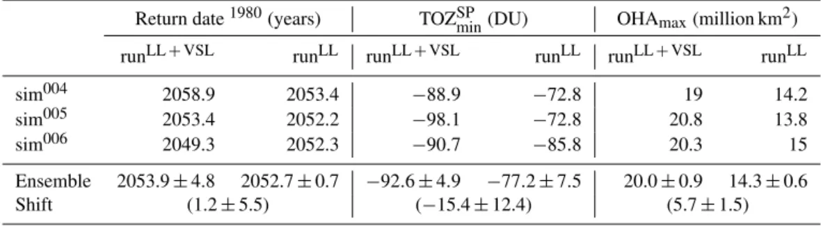
exper-Table 1.Estimation of the ozone return date, minimum ozone column within the southern polar cap (TOZSPmin)and the maximum ozone hole area (OHAmax)modelled with CAM-Chem for different simulations and ensemble members.
Return date1980(years) TOZSPmin(DU) OHAmax(million km2)
runLL+VSL runLL runLL+VSL runLL runLL+VSL runLL
sim004 2058.9 2053.4 −88.9 −72.8 19 14.2
sim005 2053.4 2052.2 −98.1 −72.8 20.8 13.8
sim006 2049.3 2052.3 −90.7 −85.8 20.3 15
Ensemble 2053.9±4.8 2052.7±0.7 −92.6±4.9 −77.2±7.5 20.0±0.9 14.3±0.6
Shift (1.2±5.5) (−15.4±12.4) (5.7±1.5)
iments and improves the overall model–satellite agreement (Fig. 2a). An individual panel for each independent simula-tion is shown in the Supplement. The temporal locasimula-tion of the minimum TOZSPoccurs simultaneously at the beginning of the 21st century in both experiments, with a minimum Octo-ber mean TOZSPcolumn of 205 and 235 DU for runLL+VSL and runLL respectively. This leads to a maximum Octo-ber TOZSP difference of−30 DU or∼14 % of the overall TOZSPduring 2003, while before 1970 the ozone differences remain practically constant and smaller than−14 DU, which represents only ∼3.5 % of TOZSP. Analysis of the global annual column (TOZGB)between model experiments dur-ing the 1960–2100 interval shows approximately −3.6 DU difference, with maximum changes reaching −5.2 DU by 1995. This represents<2 % of the annual TOZGBobserved for present time conditions and lies within the lower range of previous modelling studies for tropical and mid-latitudes over the 1960–2005 period (Sinnhuber and Meul, 2015). These calculations reveal a much larger ozone loss efficiency of VSLBrin the Antarctic ozone layer than in global or trop-ical ozone stratospheric trends.
The different stratospheric bromine loading between runLL+VSL and runLL produces a different ozone column since the very beginning of the modelled period. The
1TOZSP1980 (i.e. the difference with respect to 1980 base-line levels) during October shows a minimum for 2003 of −92 and −77 DU for runLL+VSL and runLL respectively (Fig. 2b). Hence, from the 30 DU absolute difference shown in Fig. 2a, approximately half of the ozone offset is intro-duced by the background contribution of VSLBron the global pre-ozone hole stratosphere. The additional ozone hole de-pletion (∼15 DU by 2000) induced by VSLBr is more no-ticeable between 1990 and 2010, i.e. when the stratospheric LLCl loading also maximises (see Fig. 1). This result is in agreement with Sinnhuber and Meul (2015), who reported a faster initial decrease and an overall better agreement be-tween past mid-latitude O3 trends and a model simulation
forced with the additional contribution from VSLBrsources. Much smaller impacts are modelled on the second quarter of the century when LLClconstantly decreases and other ODSs (such as CH4and N2O) increase.
Figure 3.The same as Fig. 2 but computing the average for(a, e)spring (defined as September–October),(b, f)summer (January–February), (c, g)autumn (March–April) and(d, h)winter (June–July). The monthly output for the periods where a strong dynamical transition between seasons exists has not been considered (see text for details).
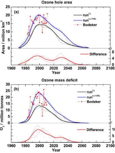
Figure 5.Temporal evolution of the ozone hole area(a)and ozone mass deficit(b)for both experiments (black for runLLand blue for runLL+VSL)on the left axis, as well as the difference between runs (red) on the right axis. Solid thick lines show the ensemble mean for each experiment, while the dashed, dotted and dashed–dotted thin lines correspond to each of the three independent simulations (sim004, sim005and sim006)for each run.
stratospheric ozone throughout the 20th century, before and after the Antarctic ozone hole formed.
Agreement between the model and observations for TOZSPand1TOZSP1980improves for all seasons when VSLBr are considered (Fig. 3). To highlight the additional chemi-cal destruction of Antarctic ozone due to biogenic bromine, the monthly output for those months where ozone depletion was dynamically controlled by the polar vortex formation and breakage (i.e. August and November–December respec-tively) were discarded. The maximum ozone difference be-tween runLL and runLL+VSL is smaller than 10 and 5 DU for summer and autumn respectively highlighting the much larger ozone depleting efficiency of the additional bromine from VSLBrsources during spring, when halogen chemistry dominates Antarctic ozone depletion. In all cases, the ozone return dates to 1980 seasonal TOZSPcolumns lay within the model uncertainties, with shorter return dates observed for the summer (∼2045) and autumn (<2040). Note also that the predicted springtime 1TOZSP1980 will not return to their
1960 values by the end of the 21st century for either runLL or runLL+VSL simulations (Figs. 2b and 3). However,
dur-ing autumn, positive1TOZSP1980 values are reached already by 2040, highlighting the different future seasonal behaviour of the Antarctic stratosphere (see Sect. 3.3).
3.2.1 Influence on the ozone hole area
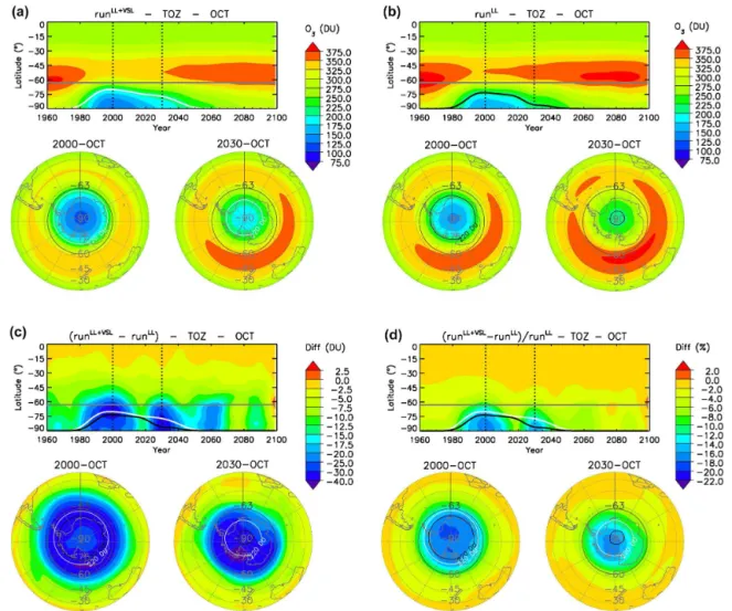
We now turn to the effect of biogenic bromine on the Antarc-tic ozone hole area (OHA). Figure 4 indicates that the inclu-sion of VSLBr produces total ozone reductions larger than 10 DU from 1970 to 2070. This enhanced depletion extends well outside the limits of the southern polar cap (63◦S) and into the mid-latitudes (see grey line in Fig. 4). Most notably, the maximum ozone depletion driven by biogenic bromine is not located at the centre of the ozone hole but on the ozone hole periphery, close to the outer limit of the polar vortex (see polar views in Fig. 4). This result has implications for assessments of geographical regions exposed to UV-B radia-tion: natural VSLBrleads to a total column ozone reduction between 20 and 40 DU over wide regions of the Southern Ocean near the bottom corner of South America and New Zealand.
Figure 5 indicates that the inclusion of VSLBr produces an extension of the maximum OHA of∼40 % by the time when the maximum ozone hole is formed (2000th decade, 1995–2005), and it almost doubles the ozone hole extension during the 2030th decade (2025–2035). However, the inclu-sion of VSLBrdrives a significantly lower impact on OHA by the time when the ozone return date to October 1980 is ex-pected to occur (2050th decade: 2045–2055). The agreement with the monthly mean ozone mass deficit (OMD) and OHA values obtained from the NIWA-BS database (Bodeker et al., 2005) is largely improved when VSLBrare considered (non-smoothed output for each independent simulation is shown in the Supplement). Most notably, the inclusion of VSLBr pro-duces a maximum enlargement of the daily OHA larger than 5 million km2, with a consequent enhancement of∼8 mil-lion tonnes to the OMD. Thus, the biogenic bromine-driven OHA enlargement is of equivalent magnitude but opposite sign to the chemical healing shrinkage estimated due to the current phase out of LLCl and LLBr emissions imposed by the Montreal Protocol (Solomon et al., 2016).
Unlike the 1980-baseline ozone return date definition (which is normalised to a preceding but independent ozone column for each ensemble), the OHA and OMD definitions are computed relative to a fixed value of 220 DU. Conse-quently, the runLL+VSLexperiment shows larger ozone hole
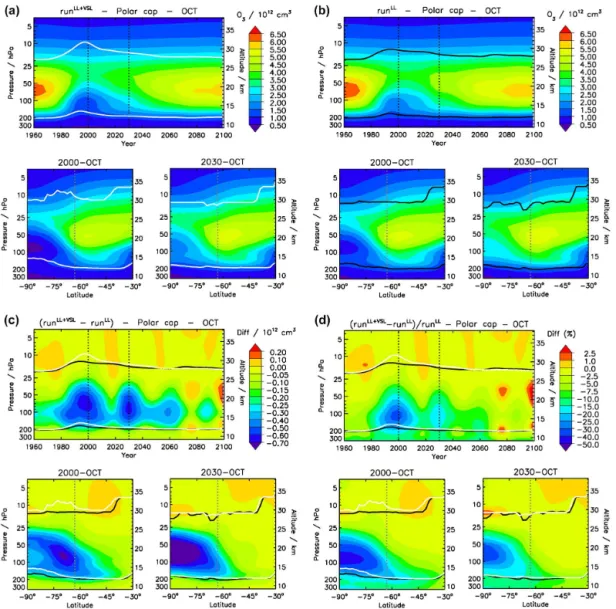
Figure 6.Temporal evolution of the ozone vertical profile averaged within the southern polar cap (O3(z)SP)for the month of October for (a)runLL+VSL,(b)runLL,(c)the absolute difference between experiments and(d)the percentage difference. The double inset at the bottom of each panel shows the October zonal mean vertical distributions during the 2000th (1995–2005 mean, left) and 2030th (2025–2035 mean, right) decades. All panels show ozone number densities (i.e. molecule cm−3)to highlight their contribution to the overall TOZ column. The lower solid line (white for runLL+VSLand black for runLL)indicates the location of the tropopause, while the higher solid line indicates the height where O3number density equals its value at the tropopause.
is still observed during 2060, i.e. after the standard 1980-return date has been reached. This indicates that the contribu-tion from VSLBrhas significant implications for the baseline polar stratospheric ozone chemistry aside from the above-mentioned impacts on ozone hole size, depth and return date. 3.2.2 Vertical distribution of the ozone hole depth Timeline analysis of the mean October ozone vertical pro-file within the southern polar cap [O3(z)SP] is presented in
Fig. 6. Typically, the deepest O3(z)SP reduction occurs in
the lowermost stratosphere, i.e. between 200 and 100 hPa (∼12 and 16 km), while during the pre- and post-ozone hole era, O3(z)SP number densities peak between 100 and
50 hPa (∼16 and 20 km). The additional O3(z)SPdepletion due to VSLBrsources is maximised precisely at the same al-titudes where the minimum O3number densities are found:
during the 2000th decade O3(z)SP densities at 100 hPa for
(see zonal panel in Fig. 6c). Above 25 hPa, O3(z)SPis not
sig-nificantly modified, with an overall VSLBr impact on ozone abundances smaller than 5 %. This can be explained by the varying importance of bromine and chlorine chemistry at dif-ferent altitudes (see Sect. 3.4). Further analysis of Fig. 6d re-veals that differences larger than 25 % at∼100 hPa are only found between 1990 and 2010, confirming that the strongest impact of VSLBr sources occurs coincidentally with maxi-mum LLClloadings (Fig. 1).
During the simulation period (i.e. 1960–2100), O3(z)SP
densities below 100 hPa are at least 10 % lower for runLL+VSL than for runLL. By 2050, when the 1980 Octo-ber return date is approximately expected to occur, the up-permost portion of the O3layer (above 50 hPa) shows strong
signals of recovery and drives the overall TOZSPreturn date,
but the O3abundance below 50 hPa is still depleted relative
to their pre-ozone hole era, mostly at high latitudes (Fig. 6d). It is only after 2080 that the O3(z)SPvertical profile is
con-sistent with the pre-ozone hole period, although O3densities
above 6×10¹²molecule cm−3 are still not recovered even by the end of the century (Fig. 6a, b). Between 2080 and 2100, inclusion of VSLBr still represents a 10 % additional O3reduction at 100 hPa, which can be explained considering
a shift from the predominant ozone destruction by chlorine to a bromine-driven depletion (whose efficiency is increased by the additional VSLBr; see Sect. 3.4).
3.3 Seasonal evolution of stratospheric Antarctic ozone
Figure 7 shows how the seasonal cycle of TOZSP has changed during the modelled period, expanding from the typical solar-driven natural annual cycle prevailing in 1960 (Fig. 7a) to the strongly perturbed anthropogenic-induced cy-cle consistent with the formation of the Antarctic ozone hole (Fig. 7c, year 2000).1TOZSPJulynormalisation in Figs. 7 and 8 was computed in respect to the TOZSPvalue in July of each year; therefore, the aperture, closure and depth of the ozone hole at each time are computed relative to the total ozone col-umn prevailing during the preceding winter. Figure 8 shows the evolution of the annual cycle of1TOZSPJulyas a function of simulated year for runLL+VSLand runLL. During the pre-ozone hole era, the typical southern hemispheric natural sea-sonality is observed, with maximum October ozone columns for runLLthat exceed the values from runLL+VSLby∼5 DU. Starting in the 1970s, the natural seasonal cycle was dis-rupted and the natural springtime maximum was replaced by a deep ozone reduction due to the ozone hole forma-tion (Fig. 7b). The maximum1TOZSPJulydifference in respect to the preceding winter reaches −95 DU for runLL+VSL (−75 DU for runLL)during October 2000 (1995–2005 aver-age), showing springtime differences greater than −30 DU (−20 DU) between September and December all the way from 1980 to 2050. The solid lines in Fig. 8 represent the temporal location of the monthly 1TOZSPJuly minimum for
Figure 7.Seasonal variation of1TOZSPJulyfor runLL+VSL (blue) and runLL (black) ensemble means at different years: (a) 1960, before the ozone first appeared;(b) 1980, where the appearance of the ozone hole produces a small TOZSPlocal minimum during spring;(c)2000, when the ozone hole depth in October maximises; (d)2040, when TOZSPminimum still appears in spring during the ozone hole recovery timeline;(e)2080, after the TOZSPglobal min-imum has already returned to autumn in its natural seasonal cycle. The solid and dashed horizontal lines highlight the local and global TOZSPminimum for each experiment.1TOZSPJulybaseline adjust-ments were computed relative to the modelled TOZSPin July of the preceding winter for each year (1TOZSPJuly=TOZSPTime−TOZSPJuly).
Figure 8. Evolution of 1TOZSPJuly as a function of the year and month. (a) runLL+VSL ensemble mean, (b) runLL ensem-ble mean and (c) absolute difference between the simulations. 1TOZSPJuly baseline adjustments were computed relative to the modelled TOZSP in July of the preceding winter for each year (1TOZSPJuly=TOZSPTime−TOZSPJuly). The solid line indicates the lo-cation of the1TOZSPJulyannual minimum for each ensemble (white for runVSLand black for runnoVSL), while the dashed lines indicate the shifts in the1TOZSPJulylocal maximums arising on each side of the springtime minimum (see Fig. 7).
the seasonal TOZSPchanges within a fully coupled climatic simulation. Note, however, that in agreement with Table 1, the modelled delay on the return date computed considering the changes in the ozone seasonal cycle also lies within the internal model variability.
The dotted lines in Fig. 8 indicate the location of the dou-ble local1TOZSPJulymaximums observed in Fig. 7b, d–e and allows the determination of how the time span between the ozone hole formation and breaking for each year changes due to VSLBr chemistry. Between the 1970s and
mid-Shift (6.3±12.2)
1980s, the seasonal development of the ozone hole for each year rapidly expanded, shifting from a starting point as early as July through a closing date during the summer (Decem-ber and January). Most notably, the seasonal ozone hole ex-tension during the first half of the century is enlarged by as much as 1 month (from January to February) for runLL+VSL between 2020 and 2040. This occurs because the additional source of VSLBr produces a deep October ozone minimum on top of the annual seasonal cycle, displacing the second local maximum in between the minima to later dates (see Fig. 7d). During the 2000th decade, the location of the sec-ond maximum, representing the closing end of the ozone hole, expands all the way to June of the following year be-cause the ozone hole depletion during October is so large that its impacts persist until the following winter is reached: the year-round depletion of 1TOZSPJuly expands from 1990 to 2010 for runLL, persisting∼7 years longer, from 1990 to 2017 for the runLL+VSL case. It is worth noting that be-cause the ozone hole seasonal extension is not tied to a fixed TOZ value (as for example 220 DU) the ozone hole seasonal duration can be computed all the way to year 2100, even af-ter the October 1980 standard ozone return date has already been achieved. These results indicate that even when LLCl and LLBr control the return date of the deepest ozone lev-els to the 1980 baseline value, the future evolution of VSLBr
sources are of major importance in determining the future in-fluence of halogen chemistry on the stratospheric Antarctic ozone seasonal cycle.
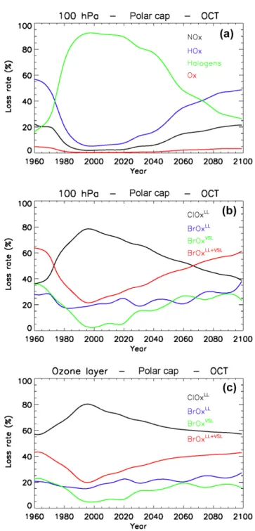
3.4 The role of chlorine and bromine ozone loss cycles (ClOLLx vs. BrOLL+VSL
x )
this work. Figure 9 shows the temporal evolution of the per-centage loss due to each cycle with respect to the total odd-oxygen loss rate as well as the partitioning between the chlo-rine and bromine components within the halogen family. In the following, note that crossed ClOx–BrOxcycles have been
included in BrOLL+x VSLlosses because both simulations in-clude identical stratospheric LLClloading but a∼5 pptv dif-ference in total bromine (see Fig. 1).
Between approximately 1980 and 2060 the dominant ozone depleting family within the springtime Antarctic ozone hole is halogens: ClOLLx +BrOLL+x VSL surpass the
otherwise dominant contribution from NOxand HOxcycles
(Fig. 9a). For example, during the year of largest ozone de-pletion (i.e. October 2003), halogens represented more than 90 % of the total odd-oxygen loss at 100 hPa, while NOx
and HOxcycles contributed∼5 % and less than 2 %
respec-tively. By 2050, when the October 1980 baseline ozone re-turn date is expected to occur, the overall BrOLL+x VSLcycles represent∼45 % of the total ozone loss by halogens occur-ring at 100 hPa (Fig. 9b) and∼35 % when integrated in the stratosphere (Fig. 9c). Even though ClOLLx losses represent as much as 80 % of the halogen-mediated ozone loss during the 2000th decade, the additional contribution from VSLBr drives bromine chemistry (BrOLLx +VSL)to dominate ozone
loss by halogens by approximately 2070. The contribution of BrOLLx +VSL cycles to ozone loss was also higher than
ClOLLx before 1975, i.e. before and during the fast increase
in anthropogenic CFCs occurred (Fig. 9b). This implies that, although anthropogenic chlorine has controlled and will con-trol the long-term evolution of the springtime stratospheric ozone hole, its overall depleting potential in the lower-most stratosphere is strongly influenced by the total (natu-ral+anthropogenic) stratospheric inorganic bromine, with a non-negligible contribution (up to∼30 %) from the biogenic VSLBroceanic sources. Within the runLLexperiment, BrOLLx cycles never surpass the contribution of ClOLLx losses, re-vealing the significant enhancement of inter-halogen ClOLLx – BrOLLx +VSLdepletion due to the additional source of natural VSLBr.
There is a clear variation in the height at which ClOxand
BrOLLx +VSL cycles produce their maximum destruction, as
well as the period of time when the losses by each fam-ily dominate with respect to the others. For example, pure ClOLLx cycles account for more than 80 % of the total
halo-gen losses above 10 hPa during the whole 21st century, while BrOLL+VSL
x cycles maximise close to the tropopause.
Fig-ure 10 shows that during the Antarctic spring, stratospheric bromine chemistry below 50 hPa has been at least as impor-tant as chlorine before and after the ozone hole era. Thus, the future evolution of stratospheric LLCllevels will control the ozone hole return date, but the role played by VSLBrby that time will be as large as the one arising from LLBr. This effect will be most evident within the lower stratospheric lev-els: bromine is globally∼60 times more efficient than chlo-rine in depleting ozone (Daniel et al., 1999; Sinnhuber et
Figure 10.Evolution of the odd-oxygen loss rate vertical profiles (VP) within the southern polar cap. The percentage contribution of each family in respect to the whole halogen loss during October is shown for(a)the ClOLLx family, and(b)the BrOLL+x VSLfamily. The inset below each VP shows the October zonal mean vertical distributions of odd-oxygen losses during the 2000th (1995–2005 mean, left) and 2030th (2025–2035 mean, right) decades. All results are for the runLL+VSLensemble. The lower solid white line indicates the location of the tropopause, while the higher solid line indicates the height where O3number density equals its value at the tropopause.
al., 2009), but its efficacy relies mostly on the background levels of stratospheric chlorine and the prevailing tempera-ture affecting the rate of the inter-halogen crossed reactions (Saiz-Lopez and Fernandez, 2016). Additionally, the extent of ClOLLx depletion within the Antarctic vortex relies on the occurrence of heterogeneous activation of chlorine reservoir species in polar stratospheric clouds, which in turn depend on ambient temperature. Then, the efficiency of BrOLLx +VSL -depleting cycles relative to chlorine is reduced in the colder lower stratosphere at high latitudes during the 2000th decade (see lower panels in Fig. 10), while the BrOLLx +VSL
contri-bution is larger at mid-latitudes and increases in importance as we move forward in time.
The representation of the ClOLLx and BrOLL+x VSL
contri-butions shown in Fig. 11 allows the address of two inter-esting features related to the seasonal and long-term evolu-tion of lower stratospheric Antarctic ozone. For any fixed year during the ozone hole era, the relative contribution of bromine chemistry reaches a minimum during austral spring, while it increases during the summer and autumn months. For example, the BrOLLx contribution to total halogen loss at 100 hPa for 2000 is 25 % during October, 65 % in Decem-ber and greater than 80 % by March. Thus, if the Antarctic return date delay is computed considering the baseline 1980 value for the autumn months, a greater impact from VSLBr is observed (see Fig. 3c). Accordingly, the evaluation of the long-term impact of ClOLLx and BrOLL+x VSL cycles on the
evolution of Antarctic ozone changes abruptly if we focus on the autumn months instead of considering the October mean. In the lower stratosphere, chlorine chemistry is dramatically enhanced during October due to the formation of the Antarc-tic ozone hole, but during summer and autumn ClOLLx losses decrease, representing less than 20 % of the total halogen loss (March mean) during the 21st century.
4 Discussion and concluding remarks
We have shown that biogenic VSLBr have a profound im-pact on the depth, size and vertical distribution of the spring-time Antarctic ozone hole. The inclusion of VSLBrimproves the quantitative 1980–2010 model–satellite agreement of TOZSP, and it is necessary to capture the lowest October mean ozone hole values. Our model results also show that, even when the maximum springtime depletion is increased by the inclusion of VSLBr, the future recovery of Antarctic ozone to the prevailing levels before 1980 is primarily driven by the evolution of the dominant LLCland LLBrsources, i.e. VSLBrsources do not significantly change the estimated re-turn date. This can be explained considering the larger im-pact of bromine chemistry during periods of high inorganic chlorine loading and the background impact of the additional bromine on the past global stratosphere. Other chemistry cli-mate modelling studies esticli-mated a decade enlargement of the expected return date based on a single member simulation
(Oman et al., 2016). Those studies considered an approxi-mate VSLBr approach, increasing the CH3Br lower
bound-ary condition by∼5 pptv, while here we performed six in-dependent simulations, including geographically distributed time-dependent VSLBroceanic sources. Note, however, that free-running ocean interactive simulations like the ones per-formed in this work possess a very large model internal variability (∼10 years difference between the shortest and largest return date for runLL+VSL); therefore, more ensemble members might be required to better address the important issue of the return date. Additional simulations including the explicit representation of VSL bromocarbons in chemistry-climate models representing the whole stratosphere would help to further reduce model uncertainties. The TOZSP min-imum and the ozone hole depth in the lower stratosphere are both increased by 14 and 40 % respectively when the addi-tional source of biogenic bromine is considered. This effect is more pronounced in the periphery of the ozone hole and within the heights of smaller ozone densities. Interestingly, biogenic bromine produces an enlargement of the OHA of 5 million km2, equivalent to that of the recently estimated Antarctic ozone healing due to the implementation of the Montreal Protocol. This large effect of oceanic VSLBr on the OHA highlights the importance of including biogenic bromine in climate assessments of the future Antarctic ozone layer. As the anthropogenic emissions of LLCland LLBrare projected to decrease in the future following the Montreal Protocol, the natural VSLBr relative contribution will repre-sent as much as 40 % of stratospheric bromine throughout the 21st century, or even more if the oceanic VSLBr source
strength and deep convection tropical injection increase in the near future (Hossaini et al., 2012; Leedham et al., 2013). Indeed, enhanced bromine BrOLL+VSL
x cycles will dominate
the chemistry of the lowermost stratosphere over Antarctica before a complete recovery of the global ozone layer from LLBrand LLClhas occurred. Hence, oceanic VSLBrpossess leverage to significantly influence the future evolution of the Antarctic ozone layer.
5 Data availability
Computing resources (ark:/85065/d7wd3xhc) were provided by the Climate Simulation Laboratory at NCAR’s Compu-tational and Information Systems Laboratory (CISL), spon-sored by the NSF. The outputs from model simulations used here are available upon request.
The Supplement related to this article is available online at doi:10.5194/acp-17-1673-2017-supplement.
support.
Edited by: Peter Hess
Reviewed by: B.-M. Sinnhuber and one anonymous referee
References
Aschmann, J. and Sinnhuber, B.-M.: Contribution of very short-lived substances to stratospheric bromine loading: uncertain-ties and constraints, Atmos. Chem. Phys., 13, 1203–1219, doi:10.5194/acp-13-1203-2013, 2013.
Aschmann, J., Sinnhuber, B.-M., Chipperfield, M. P., and Hossaini, R.: Impact of deep convection and dehydration on bromine load-ing in the upper troposphere and lower stratosphere, Atmos. Chem. Phys., 11, 2671–2687, doi:10.5194/acp-11-2671-2011, 2011.
Austin, J., Struthers, H., Scinocca, J., Plummer, D. A., Akiyoshi, H., Baumgaertner, A. J. G., Bekki, S., Bodeker, G. E., Braesicke, P., Brühl, C., Butchart, N., Chipperfield, M. P., Cugnet, D., Dameris, M., Dhomse, S., Frith, S., Lamarque, J. F., Langematz, U., Mancini, E., Marchand, M., and Michou, M.: Chemistry-climate model simulations of spring Antarctic ozone, J. Geophys. Res., 115, D00M11, doi:10.1029/2009JD013577, 2010. Bekki, S., Rap, A., Poulain, V., Dhomse, S., Marchand, M., Lefevre,
F., Forster, P. M., Szopa, S., and Chipperfield, M. P.: Climate impact of stratospheric ozone recovery, Geophys. Res. Lett., 40, 2796–2800, doi:10.1002/grl.50358, 2013.
Bodeker, G. E., Shiona, H., and Eskes, H.: Indicators of Antarc-tic ozone depletion, Atmos. Chem. Phys., 5, 2603–2615, doi:10.5194/acp-5-2603-2005, 2005.
Braesicke, P., Keeble, J., Yang, X., Stiller, G., Kellmann, S., Abra-ham, N. L., Archibald, A., Telford, P., and Pyle, J. A.: Circula-tion anomalies in the Southern Hemisphere and ozone changes, Atmos. Chem. Phys., 13, 10677–10688, doi:10.5194/acp-13-10677-2013, 2013.
Butler, J. H., King, D. B., Lobert, J. M., Montzka, S. A., Yvon-Lewis, S. a., Hall, B. D., Warwick, N. J., Mondeel, D. J., Ay-din, M., and Elkins, J. W.: Oceanic distributions and emissions of short-lived halocarbons, Global Biogeochem. Cy., 21, GB1023, doi:10.1029/2006GB002732, 2007.
Chipperfield, M. P., Dhomse, S. S., Feng, W., McKenzie, R. L., Velders, G. J. M., and Pyle, J. A: Quantifying the ozone and
ul-jections of stratospheric ozone in the 21st century, J. Geophys. Res., 112, D16303, doi:10.1029/2006JD008332, 2007.
Eyring, V., Cionni, I., Bodeker, G. E., Charlton-Perez, A. J., Kinni-son, D. E., Scinocca, J. F., Waugh, D. W., Akiyoshi, H., Bekki, S., Chipperfield, M. P., Dameris, M., Dhomse, S., Frith, S. M., Garny, H., Gettelman, A., Kubin, A., Langematz, U., Mancini, E., Marchand, M., Nakamura, T., Oman, L. D., Pawson, S., Pitari, G., Plummer, D. A., Rozanov, E., Shepherd, T. G., Shibata, K., Tian, W., Braesicke, P., Hardiman, S. C., Lamarque, J. F., Mor-genstern, O., Pyle, J. A., Smale, D., and Yamashita, Y.: Multi-model assessment of stratospheric ozone return dates and ozone recovery in CCMVal-2 models, Atmos. Chem. Phys., 10, 9451– 9472, doi:10.5194/acp-10-9451-2010, 2010a.
Eyring, V., Cionni, I., Lamarque, J. F., Akiyoshi, H., Bodeker, G. E., Charlton-Perez, A. J., Frith, S. M., Gettelman, a., Kinni-son, D. E., Nakamura, T., Oman, L. D., PawKinni-son, S., and Ya-mashita, Y.: Sensitivity of 21st century stratospheric ozone to greenhouse gas scenarios, Geophys. Res. Lett., 37, L16807, doi:10.1029/2010GL044443, 2010b.
Eyring, V., Lamarque, J.-F., Hess, P., Arfeuille, F., Bowman, K., Chipperfield, M. P., Duncan, B., Fiore, A., Gettelman, A., Gior-getta, M. A., Granier, C., Hegglin, M., Kinnison, D., Kunze, M., Langematz, U., Luo, B., Martin, R., Matthes, K., Newman, P. A., Peter, T., Robock, A., Ryerson, T., Saiz-Lopez, A., Salawitch, R., Schultz, M., Shepherd, T. G., Shindell, D., Stähelin, J., Tegt-meier, S., Thomason, L., Tilmes, S., Vernier, J.-P., Waugh, D. W. and Young, P. J.: Overview of IGAC/SPARC Chemistry-Climate Model Initiative (CCMI) Community Simulations in Support of Upcoming Ozone and Climate Assessments, SPARC Newsl., 40, 48–66, 2013.
Farman, J. C., Gardiner, B. G., and Shanklin, J. D.: Large losses of total ozone in Antarctica reveal seasonal ClOx/NOxinteraction, Nature, 315, 207–210, doi:10.1038/315207a0, 1985.
Feng, W., Chipperfield, M. P., Dorf, M., Pfeilsticker, K., and Ri-caud, P.: Mid-latitude ozone changes: studies with a 3-D CTM forced by ERA-40 analyses, Atmos. Chem. Phys., 7, 2357–2369, doi:10.5194/acp-7-2357-2007, 2007
Fernandez, R. P., Salawitch, R. J., Kinnison, D. E., Lamarque, J.-F., and Saiz-Lopez, A.: Bromine partitioning in the tropi-cal tropopause layer: implications for stratospheric injection, Atmos. Chem. Phys., 14, 13391–13410, doi:10.5194/acp-14-13391-2014, 2014.
T. G., and Waugh, D. W.: IGAC/SPARC Chemistry-Climate Model Initiative (CCMI) 2014 Science Workshop, SPARC Newsl., 43, 32–35, 2014.
Hossaini, R., Chipperfield, M. P., Dhomse, S., Ordóñez, C., Saiz-Lopez, A., Abraham, N. L., Archibald, A., Braesicke, P., Telford, P., Warwick, N., Yang, X., and Pyle, J.: Mod-elling future changes to the stratospheric source gas injection of biogenic bromocarbons, Geophys. Res. Lett., 39, L20813, doi:10.1029/2012GL053401, 2012.
Hossaini, R., Patra, P. K., Leeson, A. A., Krysztofiak, G., Abraham, N. L., Andrews, S. J., Archibald, A. T., Aschmann, J., Atlas, E. L., Belikov, D. A., Bönisch, H., Carpenter, L. J., Dhomse, S., Dorf, M., Engel, A., Feng, W., Fuhlbrügge, S., Griffiths, P. T., Harris, N. R. P., Hommel, R., Keber, T., Krüger, K., Lennartz, S. T., Maksyutov, S., Mantle, H., Mills, G. P., Miller, B., Montzka, S. A., Moore, F., Navarro, M. A., Oram, D. E., Pfeilsticker, K., Pyle, J. A., Quack, B., Robinson, A. D., Saikawa, E., Saiz-Lopez, A., Sala, S., Sinnhuber, B.-M., Taguchi, S., Tegtmeier, S., Lid-ster, R. T., Wilson, C., and Ziska, F.: A multi-model intercom-parison of halogenated very short-lived substances (TransCom-VSLS): linking oceanic emissions and tropospheric transport for a reconciled estimate of the stratospheric source gas injection of bromine, Atmos. Chem. Phys., 16, 9163–9187, doi:10.5194/acp-16-9163-2016, 2016.
Kerkweg, A., Jöckel, P., Warwick, N., Gebhardt, S., Brenninkmei-jer, C. A. M., and Lelieveld, J.: Consistent simulation of bromine chemistry from the marine boundary layer to the stratosphere – Part 2: Bromocarbons, Atmos. Chem. Phys., 8, 5919–5939, doi:10.5194/acp-8-5919-2008, 2008.
Kinnison, D. E., Brasseur, G. P., Walters, S., Garcia, R. R., Marsh, D. R., Sassi, F., Harvey, V. L., Randall, C. E., Emmons, L., Lamarque, J. F., Hess, P., Orlando, J. J., Tie, X. X., Randel, W., Pan, L. L., Gettelman, A., Granier, C., Diehl, T., Niemeier, U., and Simmons, A. J.: Sensitivity of chemical tracers to meteoro-logical parameters in the MOZART-3 chemical transport model, J. Geophys. Res., 112, D20302, doi:10.1029/2006JD007879, 2007.
Lamarque, J.-F., Kinnison, D. E., Hess, P. G., and Vitt, F. M.: Sim-ulated lower stratospheric trends between 1970 and 2005: Iden-tifying the role of climate and composition changes, J. Geophys. Res., 113, D12301, doi:10.1029/2007JD009277, 2008.
Lamarque, J.-F., Emmons, L. K., Hess, P. G., Kinnison, D. E., Tilmes, S., Vitt, F., Heald, C. L., Holland, E. A., Lauritzen, P. H., Neu, J., Orlando, J. J., Rasch, P. J., and Tyndall, G. K.: CAM-chem: description and evaluation of interactive at-mospheric chemistry in the Community Earth System Model, Geosci. Model Dev., 5, 369–411, doi:10.5194/gmd-5-369-2012, 2012.
Lee, A. A. M. and Jones, R.: Diagnosing ozone loss in the ex-tratropical lower stratosphere, J. Geophys. Res., 107, 4110, doi:10.1029/2001JD000538, 2002.
Leedham, E. C., Hughes, C., Keng, F. S. L., Phang, S.-M., Malin, G., and Sturges, W. T.: Emission of atmospherically significant halocarbons by naturally occurring and farmed tropical macroal-gae, Biogeosciences, 10, 3615–3633, doi:10.5194/bg-10-3615-2013, 2013.
Liang, Q., Atlas, E., Blake, D., Dorf, M., Pfeilsticker, K., and Schauffler, S.: Convective transport of very short lived
bromo-carbons to the stratosphere, Atmos. Chem. Phys., 14, 5781–5792, doi:10.5194/acp-14-5781-2014, 2014.
McElroy, M. B., Salawitch, R. J., Wofsy, S. C., and Logan, J. A.: Reductions of Antarctic ozone due to synergistic interactions of chlorine and bromine, Nature, 321, 759–762, 1986.
Molina, M. J. and Rowland, F. S.: Stratospheric sink for chloroflu-oromethanes: chlorine atomc-atalysed destruction of ozone, Na-ture, 249, 810–812, doi:10.1038/249810a0, 1974.
Montzka, S. A., Reimann, S., Engel, A., Krüger, K., O’Doherty, S., and Sturges, W. T.: Ozone-Depleting Substances (ODSs) and Re-lated Chemicals, in: Scientific Assessment of Ozone Depletion: 2010, Global Ozone Research and Monitoring Project-Report No. 52, Geneva, Switzerland, 2011.
Navarro, M. A., Atlas, E. L., Saiz-lopez, A., Rodriguez-lloveras, X., Kinnison, D. E., Lamarque, J., Tilmes, S., Filus, M., Harris, N. R. P., Meneguz, E., Ashfold, M. J., Manning, A. J., Cuevas, C. A., Schauffler, S. M., and Valeria Donets: Airborne mea-surements of organic bromine compounds in the Pacific tropical tropopause layer, P. Natl. Acad. Sci. USA, 112, 13789–13793, doi:10.1073/pnas.1522889113, 2015.
Oman, L. D., Douglass, A. R., Salawitch, R. J., Canty, T. P., Ziemke, J. R., and Manyin, M.: The effect of representing bromine from VSLS on the simulation and evolution of Antarctic ozone, Geo-phys. Res. Lett., 43, 9869–9876, doi:10.1002/2016GL070471, 2016.
Ordóñez, C., Lamarque, J.-F., Tilmes, S., Kinnison, D. E., Atlas, E. L., Blake, D. R., Sousa Santos, G., Brasseur, G., and Saiz-Lopez, A.: Bromine and iodine chemistry in a global chemistry-climate model: description and evaluation of very short-lived oceanic sources, Atmos. Chem. Phys., 12, 1423–1447, doi:10.5194/acp-12-1423-2012, 2012.
Saiz-Lopez, A. and Fernandez, R. P.: On the formation of tropi-cal rings of atomic halogens: Causes and implications, Geophys. Res. Lett., 43, 2928–2935, 2016.
Saiz-Lopez, A., Lamarque, J.-F., Kinnison, D. E., Tilmes, S., Or-dóñez, C., Orlando, J. J., Conley, A. J., Plane, J. M. C., Mahajan, A. S., Sousa Santos, G., Atlas, E. L., Blake, D. R., Sander, S. P., Schauffler, S., Thompson, A. M., and Brasseur, G.: Estimating the climate significance of halogen-driven ozone loss in the trop-ical marine troposphere, Atmos. Chem. Phys., 12, 3939–3949, doi:10.5194/acp-12-3939-2012, 2012.
Saiz-Lopez, A., Fernandez, R. P., Ordóñez, C., Kinnison, D. E., Gómez Martín, J. C., Lamarque, J.-F., and Tilmes, S.: Io-dine chemistry in the troposphere and its effect on ozone, Atmos. Chem. Phys., 14, 13119–13143, doi:10.5194/acp-14-13119-2014, 2014.
Salawitch, R. J., Weisenstein, D. K., Kovalenko, L. J., Sioris, C. E., Wennberg, P. O., Chance, K., Ko, M. K. W., and McLinden, C. A.: Sensitivity of ozone to bromine in the lower stratosphere, Geophys. Res. Lett., 32, L05811, doi:10.1029/2004GL021504, 2005.
doi:10.1029/1999RG900008, 1999.
Solomon, S., Kinnison, D., Bandoro, J., and Garcia, R.: Simulation of polar ozone depletion?: An update, J. Geophys. Res.-Atmos., 120, 7958–7974, doi:10.1002/2015JD023365, 2015.
Solomon, S., Ivy, D. J., Kinnison, D., Mills, M. J., Neely, R. R., and Schmidt, A.: Emergence of healing in the Antarctic ozone layer, Science, 353, 269–274, doi:10.1126/science.aae0061, 2016. Tilmes, S., Lamarque, J.-F., Emmons, L. K., Kinnison, D. E., Ma,
P.-L., Liu, X., Ghan, S., Bardeen, C., Arnold, S., Deeter, M., Vitt, F., Ryerson, T., Elkins, J. W., Moore, F., Spackman, J. R., and Val Martin, M.: Description and evaluation of tropospheric chemistry and aerosols in the Community Earth System Model (CESM1.2), Geosci. Model Dev., 8, 1395–1426, doi:10.5194/gmd-8-1395-2015, 2015.
WMO: Scientific Assessment of Ozone Depletion: 2010, Global Ozone Research and Monitoring Project-Report No. 52, Geneva, Switzerland, 2011.
WMO: Scientific Assessment of Ozone Depletion: 2010, Global Ozone Research and Monitoring Project-Report No. 55, World Meteorological Organization, Geneva, Switzerland, 2014. Yang, X., Abraham, N. L., Archibald, A. T., Braesicke, P., Keeble,