Spectrophotometric Analysis of Pigments: A
Critical Assessment of a High-Throughput
Method for Analysis of Algal Pigment
Mixtures by Spectral Deconvolution
Jan-Erik Thrane1,5*, Marcia Kyle2, Maren Striebel3, Sigrid Haande4, Merete Grung4,5, Thomas Rohrlack2, Tom Andersen5
1Department of Biosciences, Centre for Ecological and Evolutionary Synthesis (CEES), University of Oslo, Oslo, Norway,2Department of Environmental Sciences, Norwegian University of Life Sciences (NMBU),Ås, Norway,3Institute for Chemistry and Biology of the Marine Environment (ICBM), Carl-von-Ossietzky University Oldenburg, Oldenburg, Germany,4Norwegian Institute for Water Research (NIVA), Oslo, Norway,5Department of Biosciences, Section for Aquatic Biology and Toxicology (AQUA), University of Oslo, Oslo, Norway
Abstract
The Gauss-peak spectra (GPS) method represents individual pigment spectra as weighted sums of Gaussian functions, and uses these to model absorbance spectra of phytoplankton pigment mixtures. We here present several improvements for this type of methodology, including adaptation to plate reader technology and efficient model fitting by open source software. We use a one-step modeling of both pigment absorption and background attenua-tion with non-negative least squares, following a one-time instrument-specific calibraattenua-tion. The fitted background is shown to be higher than a solvent blank, with features reflecting contributions from both scatter and non-pigment absorption. We assessed pigment aliasing due to absorption spectra similarity by Monte Carlo simulation, and used this information to select a robust set of identifiable pigments that are also expected to be common in natural samples. To test the method’s performance, we analyzed absorbance spectra of pigment extracts from sediment cores, 75 natural lake samples, and four phytoplankton cultures, and compared the estimated pigment concentrations with concentrations obtained using high performance liquid chromatography (HPLC). The deviance between observed and fit-ted spectra was generally very low, indicating that measured spectra could successfully be reconstructed as weighted sums of pigment and background components. Concentrations of total chlorophylls and total carotenoids could accurately be estimated for both sediment and lake samples, but individual pigment concentrations (especially carotenoids) proved difficult to resolve due to similarity between their absorbance spectra. In general, our modi-fied-GPS method provides an improvement of the GPS method that is a fast, inexpensive, and high-throughput alternative for screening of pigment composition in samples of phyto-plankton material.
OPEN ACCESS
Citation:Thrane J-E, Kyle M, Striebel M, Haande S, Grung M, Rohrlack T, et al. (2015)
Spectrophotometric Analysis of Pigments: A Critical Assessment of a High-Throughput Method for Analysis of Algal Pigment Mixtures by Spectral Deconvolution. PLoS ONE 10(9): e0137645. doi:10.1371/journal.pone.0137645
Editor:Francois G. Schmitt, CNRS, FRANCE
Received:February 16, 2015
Accepted:August 19, 2015
Published:September 11, 2015
Copyright:© 2015 Thrane et al. This is an open access article distributed under the terms of the Creative Commons Attribution License, which permits unrestricted use, distribution, and reproduction in any medium, provided the original author and source are credited.
Data Availability Statement:All relevent data and scripts are contained within the Supporting Information of this paper.
Introduction
Quantification of phytoplankton pigments is an integral part of inland water monitoring and general experimental research involving phytoplankton. Chlorophylla(chla) concentrations, for example, are widely used by plankton ecologists as a proxy for phytoplankton biomass and for estimating primary productivity [1]. The relative concentrations of other photosynthetic and photo-protective pigments can provide valuable taxonomical and physiological informa-tion. Because pigment composition can be a reflection of taxonomic composition, presence or absence of certain marker pigments can be used to identify phytoplankton community compo-sition [2,3]. Pigment composition is also an important physiological response parameter, because the relative pigment concentrations are influenced by environmental factors such as light and nutrient availability [4].
High performance liquid chromatography (HPLC) is considered the“gold standard”for measuring pigment concentrations in plant and algal samples. HPLC can resolve most chloro-phylls and carotenoids, including their degradation products such as pheophytins and pheo-phorbides, as long as relevant pigment standards are available [5]. However, HPLC is also expensive both in terms of time and instrumentation. Running one sample takes between 20 and 30 minutes [6], and when samples contain up to 30 different unknown pigments, the costs of standards alone can be substantial. Consequently, alternative methods for pigment quantification based on spectrophotometry are still widely used [7].
Spectrophotometric assays involve solving simultaneous equations where the unknown pig-ment concentrations are modeled as a function of the measured absorbance at pigpig-ment-specific peak wavelengths [8]. At best, these methods can be used to quantify chla,bandc[9], total carotenoids, and pheophytins after acidification [10]. Although simple to perform, the results depend strongly on the empirical equation used. Highest precision is attained when using equations developed for pigment standards measured on the same instrument as for the unknown samples [11].
Recent spectrophotometric techniques use absorbance spectra from the whole visible region, with the aim of reconstructing the total spectrum as a weighted sum of all its individual component spectra [12]. One of these methods, termed the Gauss-peak spectra (GPS)
method, represents the individual pigment spectra as linear combinations of Gaussian func-tions (or“Gaussian peaks”, hereafter abbreviated GPs) [13,14]. This makes it convenient to parameterize both peak-width variations (“the widening of peaks which is observed at higher pigment concentrations due to the interaction of pigment molecules”[13]) and slight variations in pigment peak positions from one instrument to another, making the results less prone to between-instrument differences. GP spectra for 32 different chlorophylls and carotenoids were published by Küpper et al. [14], along with a spectrum fitting library for the commercial data analysis program SigmaPlot. According to the authors, the GPS method could represent a
“fast, sensitive, and inexpensive alternative to analytical pigment HPLC”.
In practice, however, the method has potential for improvement. In this paper, our goal is to make the GPS method more generally available, applicable to a wider range of ecologically rele-vant pigments, and suitable for detection of pigments in natural samples.
Materials and Methods
Gaussian peak representation of individual pigment spectra
Küpper et al. [14] represent the individual pigment absorption spectra as linear combinations of GPs, an idea we have maintained in our modified version of the method. Absorption spectra
can be efficiently represented by weighted sums of GP functions:
xðlÞ ¼X k
j¼1
bjGðl;mj;wjÞ
where G is a bell-shaped function of wavelength with a single peak located atλ=m(nm) and
with a half-peak width equal tow(nm):
Gðl;m;wÞ ¼exp 1
2
ðl mÞ2 w2
G is functionally equivalent to the Gaussian (or normal distribution) function, just without the normalization coefficient. Further statistical details can be found in the original paper, and in Naqvi et al. [12].
Instrument calibration
Küpper et al. [14] include two additional parameters,δandω, to adjust for slight variations
between spectrophotometers in spectral peak positions of pigment standards (δ; nm) and the
“widening of peaks”-effect (ω; a dimensionless constant):
Gðl;m;w;d;oÞ ¼exp 1
2
ðl m dÞ2 ow2
The original method estimates a specific value for these two parameters along with the pig-ment and background weights for every sample, making the estimation procedure non-linear. We consider these parameters to be related to the wavelength calibration and the optics of a specific instrument, and use the spectrum from a chlastandard (or similar) to estimate two instrument-specific, global values forδandω. These two (constant) values are then to be used
for all samples measured on the same instrument. This step is important, because it is a prereq-uisite for the downstream use of linear optimization. An R-script [15] for estimating instru-ment specific parameter values (calibrating the instruinstru-ment) can be found inS1 File.
Modeling of pigment and background spectra by non-negative least
squares (NNLS)
NNLS is a type of linear least squares fitting, which involves finding model parameter values that minimize the sum of squared differences between observations and model predictions. If the model is a linear weighted sum of the unknown parameters, the global minimum is found in a single step by solving an over-determined system of linear equations. On the other hand, if the model is non-linear in some of the unknown parameters, the fitting is done by an iterative search where the solution may depend on the starting values. Parameters fitted by linear or non-linear least squares can be positive or negative. This property is not desirable for fitting spectra since it is physically impossible for the spectral coefficients (that is, the weight given to each pigment in the mixture) to have negative values. NNLS is a modification of the least squares algorithm where the fitted parameters are constrained to be non-negative (0). Law-son & HanLaw-son [16] showed that the NNLS problem could be solved efficiently with approxi-mately the same computational effort as ordinary least squares. Using NNLS to fit unknown pigment mixtures thus is expected to be far more computationally efficient and numerically stable than the constrained non-linear least squares method proposed by Küpper et al. [14].
will introduce similar component spectra for modeling the background spectrum (Fig 1B). By background spectrum, we mean any light attenuationnotattributable to pigment absorption; mainly scattering by particles in the sample, or absorption by non-algal components extracted from the sample. Küpper et al. [14] modeled the background spectrum with a 3-parameter decreasing exponential function. As a consequence this turns the spectrum-fitting problem into a non-linear one, even when using NNLS to fit the mixture component spectra. The absor-bance spectrum of the non-algal background is generally found to be smooth and featureless, with an exponential decrease with increasing wavelength.
We observe that as with any continuous function, the decreasing exponential can be approx-imated by a Taylor polynomial. In other words, we can represent the decreasing exponential background spectrum as a linear combination of power functions of wavelength. If we con-struct background basis functions as powers of a linear function decreasing from 1 to 0 over the wavelength range of the fit, the coefficients of a Taylor expansion of the negative exponen-tial will have non-negative coefficients. Consequently, we can use NNLS to fit both the back-ground spectrum and the pigment mixture coefficients. In practice this is done by running NNLS with an augmented design matrixX= [XpXb] consisting of the pigment spectrum model
matrix (Xp) and a background model matrix (Xb) whose columns are power basis functions.
We let the first column ofXbconsist of ones, such that the fitted coefficient for this column will
represent a possible constant baseline offset in the spectrum. The coefficients fitted by NNLS will thus consist of two groups, of which the former represent the pigment mixture weights while the latter can be used to construct the fitted background spectrum.
We then used the following calculations to fit the data using NNLS (for simplicity, we left out the background components from the description). If we have a mixture ofnpigments with known absorbance spectraxi(λ),i= 1. . .nat wavelengthsλ(nm), then the spectrum of
the mixturey(λ)will be a weighted sum of the individual component spectra:
yðlÞ ¼a
1x1ðlÞ þa2x2ðlÞ þ. . .þanxnðlÞ
If the component spectra are normalized to unit maximum peak absorbance, the weights (ai) will be equal to the product of pigment concentration (ci; g L-1) and the pigment’s
weight-specific absorption coefficient at the maximum peak wavelength (ui; L g-1cm-1):ai=ciui. In
matrix notation, this mixture model can be written as:
yðlÞ ¼XðlÞa
WhereX(λ) = [x1(λ),x2(λ),. . .xn(λ)] is a matrix with columns that are the component pigment
spectra, anda= [a1,a2,. . .,a
n]Tis the column vector of mixture weights. Estimating the pigment
composition of an unknown mixture by ordinary least squares then reduces tofinding a mix-ture weight vectorâsuch that the L2-norm of the residualskyðlÞ XðlÞ^ak2is minimized.
Remembering that the mixture weights cannot be negative, we minimize the residual L2norm subject to the non-negativity constraintâ>0 by the NNLS algorithm.
where the weights depend on the composition of the pigment extract. The weighted component spectra are summed to obtain the total pigment spectrum (E) and the total background spectrum (F). Adding together the pigment and background spectra yields the total spectrum of the extract (G).
Calculation of individual pigment concentrations
Concentration of pigmentiin the extract (mg/L) was further calculated as:
ci¼1000 ai ui
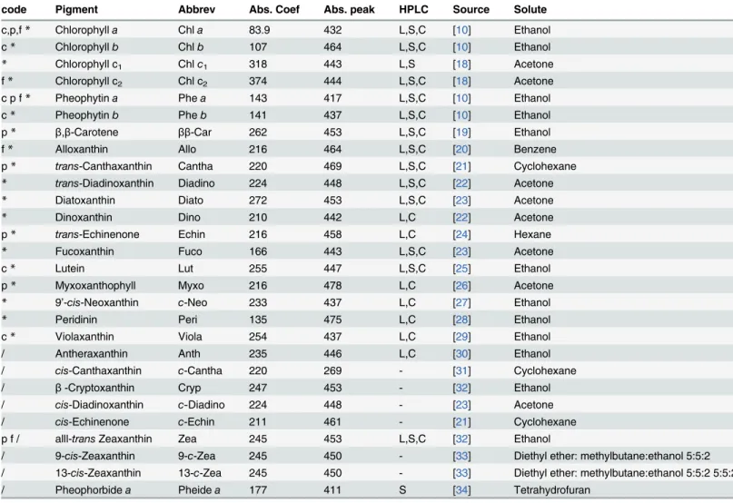
Specific absorption coefficients (L g-1cm-1) were obtained from Appendix F in Phytoplank-ton pigments–characterization,chemotaxonomy and applications in oceanography[17]. If a
coefficient determined for ethanol was available, it was used. If not, we used the value recom-mended by [17] even if it was from another solvent. Coefficients and original references ([10],
[18–34]) are listed inTable 1.
Development of a core set of pigments for unknown samples
Küpper et al. [14] presented GP parameters describing the absorption spectra of 12 chloro-phylls and 20 carotenoids. We updated this list with four new pigments from common phyto-plankton species: peridinin (peri), dinoxanthin (dino), alloxanthin (allo), and pheophorbidea (pheidea; refer toTable 1for pigment names and abbreviations). After obtaining the absor-bance spectra for the new pigments (described below), they were fitted as sums of GPs (seeS2 Filefor an R-script describing the estimation). We also obtained new spectra and GPs parame-ters for chlaandbin ethanol. We removed eight uncommon pigments from the original list of Küpper et al. [14], including all zinc, copper and cadmium chlorophylls, diadinochrome, and aurochrome, to obtain a list of GP parameters for 28 of the normally occurring pigments in natural phytoplankton communities.
A general problem with spectral deconvolution techniques, also mentioned by Küpper et al. [14], is aliasing. In other words, since some pigments have extremely similar absorption spec-tra, there might exist several weighted combinations of component spectra that can add up to approximately the same total spectrum. When measuring samples of unknown community composition (for example lake samples), many pigment component spectra need to be included to capture what might be present. However, if spectra are easily confused, it might be better to only include a“core set”of pigments that are less prone to aliasing for such samples. We made decisions on which pigments to include in such a“core”based on a Monte-Carlo simulation of each pigment’s identification error rate.
The simulation was done as follows: A simulated pigment mixture was developed by ran-domly selecting four pigments and combining their GP spectra to create a test sample. This spectrum was scaled to a peak absorbance of 1 and perturbed with normally distributed white noise with a certain standard deviation (Sd). The simulated mixture-spectrum was then fitted by NNLS using a pigment spectrum model matrix (Xp) containing all the 28 different pigment
spectra. These steps were repeated 100,000 times and used to calculate frequencies of detecting a pigment that was not present in the test sample (false positive), and of failing to detect a pres-ent pigmpres-ent (false negative). This procedure was again repeated for 10 differpres-ent values of Sd (0.00001, 0.00003, 0.00007, 0.0002, 0.00055, 0.0015, 0.0041, 0.011, 0.03, 0.082, and 0.22). Increasing the standard deviation of the errors in a stepwise fashion made it possible to assess both the algorithm’s sensitivity to experimental error, and the differences between pigments in error rates. The R scripts used for these simulations are included inS3 File.
Sample preparation and analysis of absorbance spectra
overnight at 4°C in the dark. All lakes were located on public land, and prior to sampling per-mission was obtained from local Norwegian municipalities: Aremark, Arendal, Aurskog-Høland, Trøgstad, Bergen, Bjerkreim, Bjugn, Bærum, Oslo, Elverum, Fet, Rælingen, Enebakk, Trøgstad, Flesberg, Fræna, Fusa, Gjesdal, Grue, Halden, Hemne, Hjelmeland, Hof, Hurum, Jev-naker, Gran, Søndre Land, Dokka, Jølster, Krødsherad, Flå, Larvik, Levanger, Lunner, JevJev-naker, Table 1. Pigment list.
code Pigment Abbrev Abs. Coef Abs. peak HPLC Source Solute
c,p,f* Chlorophylla Chla 83.9 432 L,S,C [10] Ethanol
c* Chlorophyllb Chlb 107 464 L,S,C [10] Ethanol
* Chlorophyll c1 Chlc1 318 443 L,S [18] Acetone
f* Chlorophyll c2 Chl c2 374 444 L,S,C [18] Acetone
c p f* Pheophytina Phea 143 417 L,S,C [10] Ethanol
c* Pheophytinb Pheb 141 437 L,S,C [10] Ethanol
p* β,β-Carotene ββ-Car 262 453 L,S,C [19] Ethanol
f* Alloxanthin Allo 216 464 L,S,C [20] Benzene
p* trans-Canthaxanthin Cantha 220 469 L,S,C [21] Cyclohexane * trans-Diadinoxanthin Diadino 224 448 L,S,C [22] Acetone
* Diatoxanthin Diato 272 453 L,S,C [23] Acetone
* Dinoxanthin Dino 210 442 L,C [22] Acetone
p* trans-Echinenone Echin 216 458 L,C [24] Hexane
* Fucoxanthin Fuco 166 443 L,S,C [23] Acetone
c* Lutein Lut 255 447 L,S,C [25] Ethanol
p* Myxoxanthophyll Myxo 216 478 L,C [26] Acetone
* 9’-cis-Neoxanthin c-Neo 233 437 L,C [27] Ethanol
* Peridinin Peri 135 475 L,C [28] Ethanol
c* Violaxanthin Viola 254 437 L,C [29] Ethanol
/ Antheraxanthin Anth 235 446 L,C [30] Ethanol
/ cis-Canthaxanthin c-Cantha 220 269 - [31] Cyclohexane
/ β-Cryptoxanthin Cryp 247 453 - [32] Ethanol
/ cis-Diadinoxanthin c-Diadino 224 448 - [23] Acetone
/ cis-Echinenone c-Echin 211 461 - [21] Cyclohexane
p f / alll-transZeaxanthin Zea 245 453 L,S,C [32] Ethanol
/ 9-cis-Zeaxanthin 9-c-Zea 245 450 - [33] Diethyl ether: methylbutane:ethanol 5:5:2
/ 13-cis-Zeaxanthin 13-c-Zea 245 450 - [33] Diethyl ether: methylbutane:ethanol 5:5:2 5:5:2
/ Pheophorbidea Pheidea 177 411 S [34] Tetrahydrofuran
Pigments with abbreviations (Abbrev) used for the modified Gaussian Peak Spectra (GPS) method described in this paper. Specific absorption coefficients (Abs. Coef; L g-1cm-1) and corresponding absorbance peaks (Abs. Peak; nm) are given. The HPLC column indicates if a standard for the pigment was included in the HPLC analysis of the sample
L: lake samples S: sediment C: cultures.
Pigments (code) are identified as follows: *=“core”set
c = culture specific set (Chlamydomonas p = Planktothrix
f= Cryptomonas
Pigments not included in thefinal“core”set (/) due to high error rates.
Løten, Marker, Nord-Aurdal, Nord-Aurdal, Vestre Slidre, Oppegård, Ringerike, Ringsaker, Rømskog, Sandefjord, Larvik, Sandnes, Skaun, Skodje, Haram, Stange, Stavanger, Randaberg, Strand, Stryn, Sveio, Søndre Land, Sør-Odal, Nord-Odal, Tokke, Tokke, Kviteseid, Trysil, Tys-vær, Vestre Toten, Vindafjord, Vinje, Volda, Voss, Ørsta, Åmot, Trysil, Åsnes. No endangered species are present in any field site.
Samples for sediment pigment analyses were obtained from a core taken at 25 m depth in Lake Steinsfjorden (60°05'43.17"N 10°19'30.84"E). The core was sliced in 1 cm sections starting from the sediment surface and maintained at -20°C. Prior to extraction, the samples were freeze-dried; subsamples were placed into pre-weighed 5mL polypropylene vials and re-weighed. Ethanol (96%) was added by pipette and the entire tube–sample and extraction solution–was again weighed to obtain the amount of ethanol used for extraction. Extraction volumes were then calculated from weights, assuming a mass density of 96% ethanol of 0.81 g mL-1. Sediment to extraction volume was approximately 0.4
–0.6 g mL-1. Samples were thor-oughly mixed by vortex and followed by gentle centrifugation to ensure all sediment remained in contact with the solvent. The samples were then extracted for 20 hours in the dark at 4°C.
Cultures ofPlanktothrix(including both red and green strains), a filamentous cyanobacte-rium, were obtained from the Norwegian Institute of Water Research Culture Collection and harvested during the exponential growth phase from batch cultures grown at 20°C under 3–5μmol PAR m-2s-1, in Z8 medium. Aliquots of the cultures were centrifuged, and pellets
transferred to vials and lyophilized. The freeze-dried samples were weighed, and then extracted in 96% ethanol overnight at 4°C. Cultures of the chlorophyteChlamydomonas reinhardii (strain cc-1690) and the cryptophyteCryptomonas ozoliniiwere harvested at the end of the exponential phase from batch cultures grown at a light level of approximately 35μmol
PAR m-2s-1. Ten milliliters of each culture was filtered onto 25 mm Whatman GF/F filters, and stored at -80°C until extraction in 3 mL 96% ethanol overnight at 4°C.
High-throughput absorbance measurements. All absorbance (that is,log10
I0 I
) measure-ments were made in a Synergy MX plate reader (BioTek instrumeasure-ments, Vermont, USA) and all spectral scans were recorded between 400 and 700 nm using one nm resolution. Because the path length for a top-reading plate reader is dependent on the volume of liquid in the chamber, the path length (l, cm) in the micro-well was calculated as v/a, wherev(cm3) is the volume of the sample anda(cm2) is the area of the well bottom. Absorbance was, however,not normal-ized to unit cm-1until after pigment weights were estimated by NNLS. The absorbance spectra were saved as a data matrix with one sample spectrum per column, and used as input to the R-script in the downstream analysis. Note that the absorbance of a blank (plate and solvent absorbance) was not subtracted. Instead, this absorbance was modeled as a part of the general background, as described above.
For the spectral scans, different well plates and well volumes were used depending on sam-ple-type. Sediment extracts utilized 96-well flat bottom clear polypropylene plates (Greiner bio one #655201) with 330μL sample per well. For cultures, 96-well polystyrene plates (Greiner bio
one,μClear F-bottom) with 330μL of sample volume were used. For natural lake samples, we
used 48-well polystyrene plates (Nunc flat bottom, Thermo scientific) with 750μL per sample.
To assess possible background effects of different micro-plate material, we utilized one extract from a single culture (Planktothrix) and scanned using three different types of 96-well-plates: clear polystyrene (Greiner bio one), white polystyrene with clear bottom (Greiner bio one,μClear, F-bottom), and clear polypropylene (Greiner bio one, F-bottom). Pigment and
Use of ethanol as solvent. Küpper et al. [14] used acetone for pigment extraction. Because acetone is highly volatile, samples evaporated rapidly from our wells and made a full 96 well plate difficult to measure in one run. Another possible extraction solution was methanol, also commonly used in pigment analysis. However, both acetone and methanol have negative effect on pipettes [36] and they require the use of polypropylene micro-plates. For these reasons, the solvent was changed to 96% ethanol. Ethanol has been shown to be an effective extraction sol-vent in pigment analysis [36]. While each solvent has its own virtue, we selected ethanol to allow for ease of 96 well plate usage and for occupational safety. No further comparison of extraction efficiency was done for this study. However, replicate samples of one culture (Chlamydomonas) were extracted using either ethanol or acetone and then analyzed using either the software from Küpper et al. [14] or our modified method to compare concentration differences between the original GPS and modified-GPS.
HPLC analyses. Replicate samples from the natural lake and culture samples were ana-lyzed by HPLC at Wassercluster Lunz (Austria). Pigments were extracted in 90% acetone. To improve extraction, samples were combined with quartz sand, vortexed, and sonicated for 30 minutes on ice. Samples were stored at 4°C in the dark for 24h before analysis. Analytical protocol and HPLC system was the same as in Schagerl & Künzl [37]. Sediment pigments were analyzed by HPLC at the Norwegian Institute for Water Research (NIVA). Pigments were extracted from freeze-dried samples in 90% acetone in for 4h. One minute of sonication was applied to improve extraction. Samples were centrifuged before the supernatant was injected into a HPLC system. Analytical protocol and HPLC system was the same as in Hobaek et al. [38]. Pigment standards used for detection are listed inTable 1, for both labs.
Measurement of additional pigment spectra. Pure standards, including chla (Sigma-Aldrich), allo (DHI; Hørsholm, Denmark), and pheide a (DHI), were dissolved in 96% ethanol. Absorbance spectra (400–700 nm, every nm) were recorded using the plate reader and clear polypropylene microwell plates (Greiner bio one, F-bottom) containing 300μL sample per
well. The absorbance of a well with 96% ethanol was subtracted. Spectra for chlb(95% etha-nol), dino (ethanol, unknown %), and peri (acetone, unknown %) were digitized from Lich-tenthaler [10], Jeffrey et al. [39], and Roy et al. [17], respectively.
Statistical analysis
R-scripts and data. R-scripts were developed for our modified-GPS method and can be found inS4 File,S5File. These folders include the data and scripts used to obtain the results from the sediment and natural lake samples, respectively. Each folder includes 1) the main script with two accompanying sample text files consisting of sample information and sample scans and 2) the“pigment.function.R”script with two accompanying text files. For example,
theS5 File(Lake) folder includes a main script for analysis (“Lake.R”) and two text files
con-taining absorbance spectra from 75 lakes (“Lake abs spec.txt”) and sample IDs with filtration volumes (“Lake sample ID.txt”). The main script is used to decompose the measured spectra into pigment and background components, and to calculate pigment concentrations. The script“pigment.function.R”must be present in the folder so that it can be loaded with the main script (using the R function“source”) to make the fitting functions available to the user. In short, these functions, which are further described inS1 Text, include the“pigment.basis”
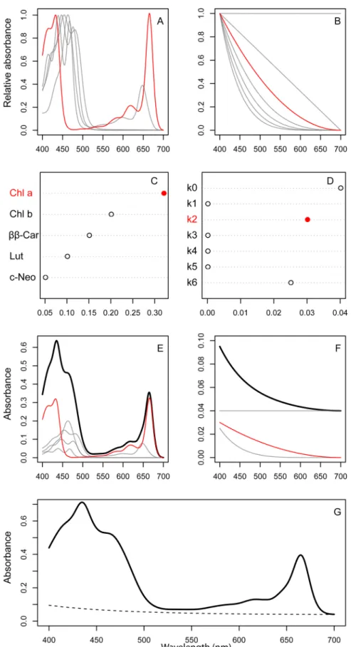
function that generates the pigment basis spectra from their GP parameters (Fig 1A). The
spectrum”, and“fitted.spectrum”use the results from“pigment.fit”as input, and calculates the total pigment spectrum (Fig 1E, black line), the total background spectrum (Fig 1F, black line; g, dashed line), and the total fitted spectrum (Fig 1G, solid line), respectively. The last function
“pigment.concentration”also uses“pigment.fit”as input, as well as a path-length (L, cm) for absorbance normalization. It yields concentrations of all the detected pigments as mg L-1in the extract. Note that any conversion to sample concentrations (for exampleμg L-1of lake water),
must be done afterwards. The“pigment.function.R”script needs two text files that include the GP parameters (“gaussian.peak.parameters.txt”) and the weight-specific absorption coefficients (“specific absorption coefficients.txt”). Both of these must be contained in the same folders as the other R files.
Comparing pigment concentrations with HPLC results. Pigment concentrations obtained by the modified-GPS method were compared with results from HPLC. In the first level of pigment comparison, we pooled all chlorophylls and all carotenoids from both the modified-GPS and HPLC results. The resulting total chlorophyll (total chl) and total caroten-oid (total car) concentrations were compared using linear regression within the natural lake samples (n = 75) and sediment samples (n = 40).
Rather than comparing each pigment by correlation or linear regression, we used principal component analysis (PCA) to compare the results from the two methods on single-pigment level. We did so because not all pigments were present in both methods (not all HPLC stan-dards were available as GP spectra, and vice versa), and because of the tendency of the GPS methods to confuse carotenoid spectra. If the two methods identified similar gradients in pig-ment composition, the PCA axes calculated from the two pigpig-ments vs. sample matrixes should be correlated. We used Kendall’sτas a measure of correlation due to non-normal axis scores.
For the PCA on natural lake samples, some pigments were combined. These included chla with phea, chlbwith pheb, and chlc1withc2which then created three different totals (tot chl
a, tot chlb, and tot chlc). All pigment concentrations were normalized to the total chla con-centration. In the PCA on sediment samples, all pigment concentrations were normalized to tot chla, calculated as the sum of chlaand phea. Some pigments were not present as both GP spectra and HPLC standards, such asα-carotene, 19’-butanoyloxyfucoxanthin, crocoxanthin, and lycopene, which were present as HPLC standards, but not as GP spectra. These pigments were omitted from the PCA. For culture samples, individual pigment concentrations were compared directly. To assess the method’s ability to reconstruct measured absorbance spectra, we calculated root mean squared errors (RMSEs) between observed and fitted spectra.
The extent of background attenuation. We assessed the contribution of the background spectrum to the total spectrum in natural lake and sediment samples by fitting absorbance spectra with the solvent blank subtracted as weighted sums of the component spectra. Any background signal estimated for these spectra should be due to either scattering, or absorption by non-algal components extracted from the filter. In addition, we related the extent of these background spectra (the integral under the spectrum from 400–700 nm) to the amount of par-ticulate organic carbon (POC) and chlain the natural lake samples (described in [35]). We hypothesized that a high POC:chlaratio could lead to an increased background contribution.
Results
Aliasing and selection of a core pigment set
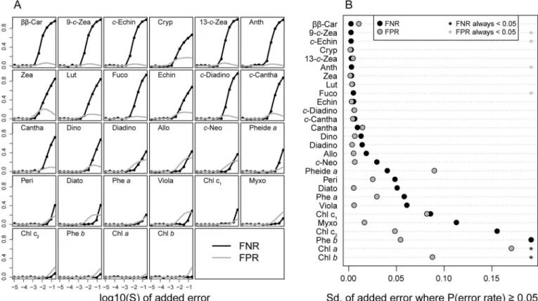
The results from the Monte-Carlo simulation showed that false positive and false negative rates increased with simulated measurement noise (Sd) (Fig 2A). The false negative rates were gener-ally higher than the false positive rates (Fig 2B). At low Sd values (<~ 0.001) most pigments
were correctly identified, but some carotenoids (zea and cryp) were falsely identified even at Sd<0.001. At Sd values between 0.001 and 0.01, most carotenoids had false positive rates
close to 0.1 and false negative rates between 0.1 and 0.7 (Fig 2A), indicating a strong tendency for aliasing for these pigments. All chlorophylls had low error rates except at the highest Sd val-ues (well above 0.01). Such noisy spectra are, however, not realistic unless the pigment concen-tration is very low.
The results from the simulation was used to identify a selection of“core pigments”that would be the most likely pigments to find in a natural sample, as well as having a high probabil-ity of identification. For instance, zea and cryp, were removed due to their very high false posi-tive rates and high correlation withββ-Car (r = 0.999). 19 pigments were selected for the final core (seeTable 1) and further tested by an additional Monte-Carlo simulation indicating that these pigments were identifiable (S1 Fig).Table 1summarizes the original 28 pigments tested and lists those that were removed to obtain the core set. GP parameters for the core pigments
Fig 2. Results from the Monte-Carlo simulation of pigment detectability.In A), the course of the false negative rate (FNR; black line) and the false positive rate (FPR; grey line) as the standard deviation of the random error is increased (see text), is shown for each pigment. The pigments were sorted from highest to lowest FNR, also shown in B). Here, we estimated how high the added random noise had to be for the FNR and FPR to exceed 0.05 (5%). Black dots represent the standard deviation of this random error for the FNR, the grey dots for the FNR. Asterisks mean that the FNR (black asterisks) or FPR (grey asterisks) never exceeded 5% for that pigment.
are used as default in the functions contained in“pigment.function.R”. Note, however, that when a specific pigment profile is expected (such as for samples from known algal cultures), it is possible to adjust the list of candidate pigments. This can be easily accomplished in the R functions (seeS1 Textfor an example). As noted in Küpper et al. [14], removal of unexpected pigments in a particular research question would further improve the quality of the estimates.
Test of performance by the modified-GPS method
For the modeling of sediment and natural lake samples we use the core set of candidate pig-ments, while culture samples were modeled using an appropriate, species-specific subset (see
Table 1).
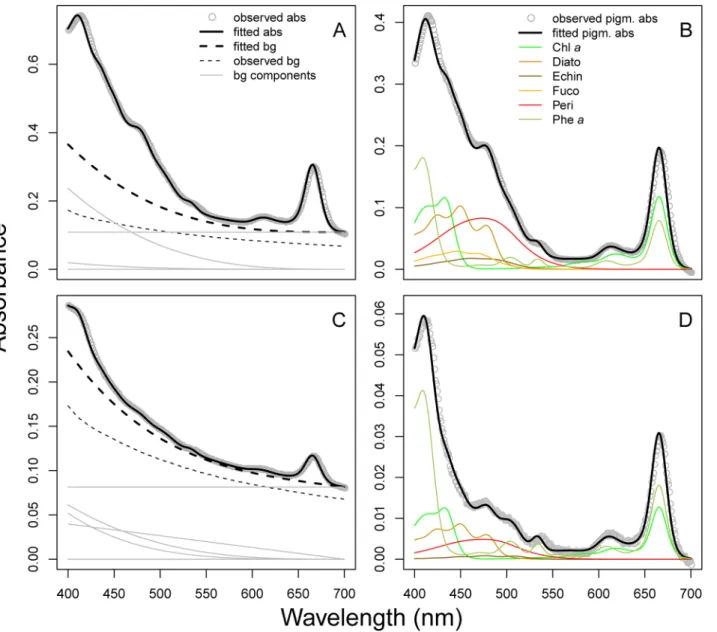
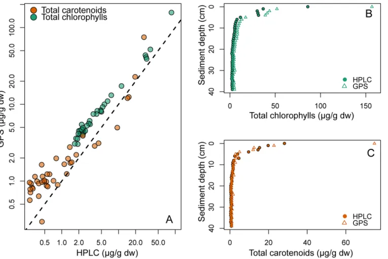
Sediments. The sediment absorbance spectra fitted by NNLS were very similar to the observed absorbance spectra (Fig 3). Samples deeper than approximately 5 cm had very low pigment-to-background ratio (Fig 3C), but distinct pigment spectra were still apparent after subtracting the modeled background spectrum (Fig 3D). Root mean squared error (RMSE) val-ues spanned from 0.0004 to 0.005 with a mean of 0.00095. Concentrations of total chl (calcu-lated as the sum of all chlorophylls and pheophytins) and total car (sum of all xanthophylls and carotenes) estimated by modified-GPS were significantly correlated with HPLC (Fig 4A, log-log relationships: r2= 0.99 for total chl, and 0.86 for total car, both p-values<0.0001,
n = 40), and both methods captured the expected decline in pigment concentrations with sedi-ment depth (Fig 4B and 4C). Absolute concentrations were generally slightly higher in the modified-GPS than HPLC for both pigment types (Fig 4). This, however, might be explained by differences in extraction procedure between the two methods. The largest difference in total car between methods was observed at low carotenoid concentrations (Fig 4A). The two first PCA axes (figure not shown) estimated from the modified-GPS results were significantly corre-lated with the corresponding axes from HPLC (PCA1: Kendall’sτ= 0.47, p<0.001; PCA2:
Kendall’sτ= 0.45, p<0.001), indicating significant similarity between the pigment
composi-tion gradients captured by the two methods. Interestingly, chlaand its degradation product pheawere well separated by modified-GPS as indicated by the high correlation between meth-ods for these pigments (r2= 0.97 for both pigment pairs). Many carotenoids were, nevertheless, clearly misidentified compared to HPLC.
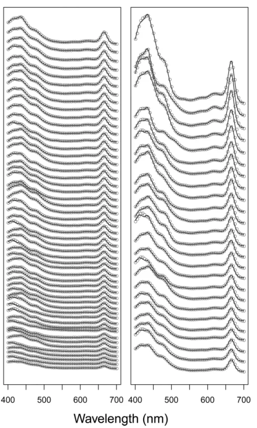
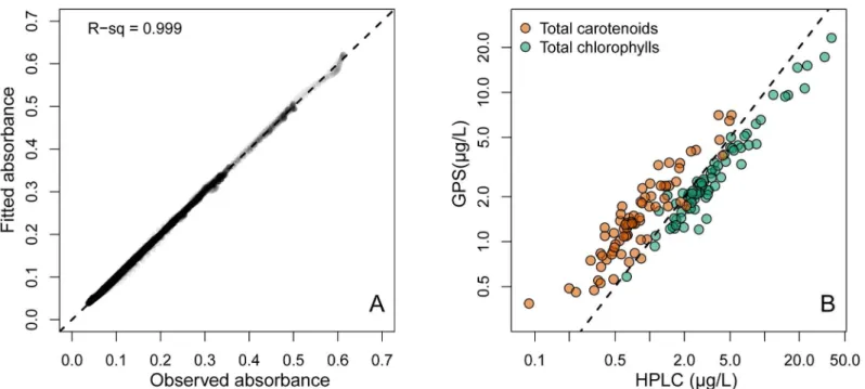
Natural lake samples. Spectra fitted by NNLS were again very similar to the observed nat-ural lake sample pigment spectra (Fig 5andFig 6A), with RMSE values spanning from 0.0004 to 0.005 (mean = 0.0013). Estimates of total chl and total car by modified-GPS were highly cor-related with HPLC (Fig 6B, log-log relationships: r2= 0.94 for total chl, and 0.84 for total car, both p-values<0.0001, n = 75). The modified-GPS method, however, underestimated total
chl and overestimated total car (Fig 6B), compared to HPLC.
There was a significant correlation between scores on PCA axis 1 from the two methods (Kendall’sτ= -0.2, p<0.05; notice that signs of PCA axes are arbitrary and without
conse-quence), but not between PCA axis 2 scores. This indicates that the pigment compositions were similar for modified-GPS and HPLC, but that many individual pigment estimates, espe-cially among carotenoids, were dissimilar.
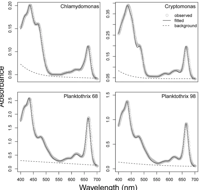
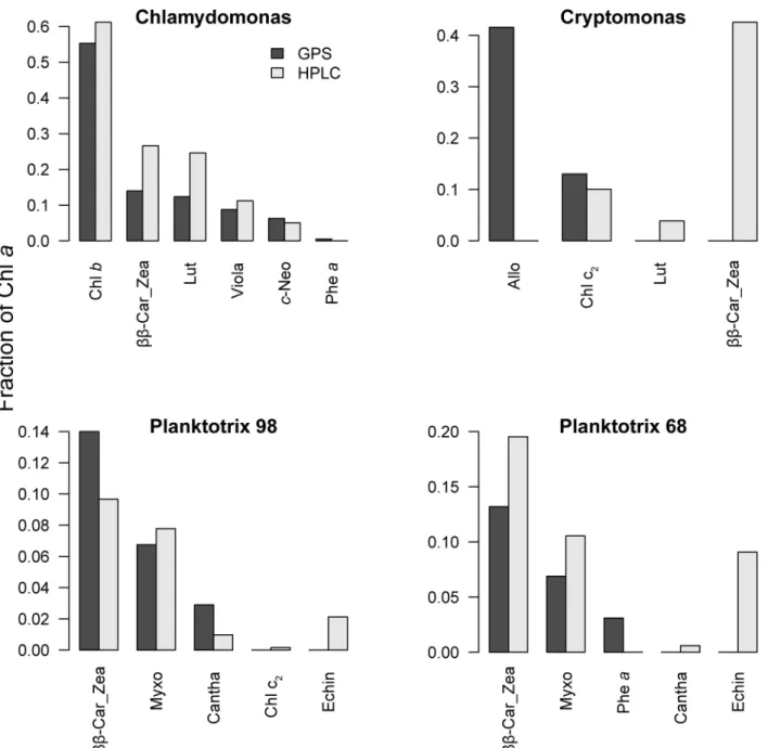
Phytoplankton cultures. Observed and fitted spectra (Fig 7) were similar, with RMSE val-ues ranging from 0.0008 forChlamydomonasto 0.019 (Fig 7A) forPlanktothrix 68(Fig 7C). Before comparing individual pigment estimates, we normalized all concentrations to chlato avoid differences in extraction efficiency between methods. Due to the similarity between the zea andββ-Car spectra, these two pigments were merged and presented asββ-Car.Zea.
Concentrations of chlbandc2were in good agreement with HPLC inChlamydomonasand
in thePlanktothrix98 strain (Fig 8C), even though this pigment should not be present in cya-nobacteria. A small amount of pheawas identified by the modified-GPS inChlamydomonas andPlanktothrix98, but standards for this pigment were not included in the HPLC analysis. For carotenoids, we observed larger differences between methods. In theChlamydomonas sam-ple concentrations were reasonably similar (Fig 8A). InCryptomonas, modified-GPS identified allo, which is a cryptomonad-specific pigment, while HPLC identifiedββ-Car.Zea as the
dominant carotenoid (Fig 8B) based on the sample absorbance peaks at 427, 454, and 483 nm Fig 3. Absorbance spectra measured on sediment extracts.Data from two depths in the sediment column is shown: A) and B) are from the upper cm, C) and D) from 5 cm below the sediment surface. The difference in absorbance between the two samples can be attributed to lower pigment concentrations deeper in the sediment. A & C) The measured total absorbance spectrum (grey dots) overlaid with the fitted total absorbance spectrum obtained using the modified-GPS method (solid black line). Background spectra (scattering and/or absorbance by non-algal pigment) are represented by dotted lines; the thick line being the modelled background, while the thin line is the measured blank spectrum (absorbance of a well filled with 96% ethanol). Thin grey lines represent the different component spectra making up the modelled background spectrum. In B) and D), the modelled background spectrum is subtracted from the total spectrum, yielding only pigment absorbance. The spectra of the individual pigments recognized by the modified-GPS method are shown in colour.
(482 in one replicate sample). These peaks were closest to the zea pigment standard peaks (428, 454, 480.9), but also close to the allo peaks (431, 455, 485). A small amount of lut was also iden-tified by HPLC. In both strains ofPlanktothrixcultures, there was an inconsistency between methods for the carotenoid echinenone that was detected by HPLC, but not apparent in the modified-GPS. The comparison ofChlamydomonaspigment concentrations for samples extracted with either acetone and the Küpper et al. [14] method or ethanol with our modified-GPS were very consistent (data not shown).
Direct comparison of GPS and modified-GPS. Testing of the two methods using a single culture of the green algaeChlamydomonaswith different extraction solutions resulted in no statistical differences (data not shown). When the Küpper et al. [14] method was used on the acetone extracts and our version on the ethanol extracts, the results from this test were very similar, indicating that each method works well on the correct solvent.
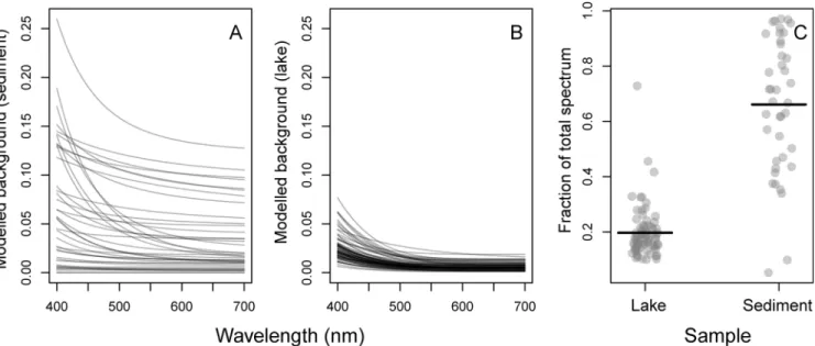
The background attenuation signal. The modified-GPS method estimated a significant background signal on all the blank-corrected spectra for both sediment (Fig 9A) and lake (Fig 9B) samples. The fraction of the total spectrum constituted by the background spectrum, calcu-lated by dividing the integral under each background spectrum (bgint) by the integral under the Fig 4. Total chlorophylls and total carotenoids from sediment.A) Concentrations (μg pigment per gram sediment dry weight) of total chlorophylls (green) and total carotenoids (orange) as estimated by modified-GPS (y-axis) and HPLC (x-axis). The dotted line shows the 1:1 relationship. Note that both axes are log-transformed due to the large variation in concentrations. Pigment concentrations decreased with sediment depth, both total chlorophylls (B) and total carotenoids (C).
Fig 5. Observed and fitted spectra from lake samples.Absorbance spectra from the 75 natural lake samples (not normalized to unit path-length) plotted as grey dots. For clarity, spectra are ordered from lowest to highest maximum absorbance, and dots plotted only for every fifth nm. A vertical offset is added between each spectrum, therefore no units on the y-axis. Fitted spectra are added as black lines.
corresponding total (pigment + background) spectrum, was generally higher and more variable in the sediment samples compared to the lake samples (Fig 9C). A linear regression with log (bgint) as a function of log(POC) and log(chl a) revealed a significant positive relationship with chla(p<0.0001), but a non-significant effect of POC using natural the lake data (n = 75, r2=
0.48). This indicates a contribution to the background from the amount of algae on the filter, possibly scattering by algae-related particles. No effect of POC might indicate that absorption by non-algal compounds matter is less important.
Discussion
Comparing the GPS with other spectrophotometric methods
Classical multi-wavelength spectrophotometric methods (e.g., [7], [8], [9]) all depend on sub-tracting a solvent blank or the absorbance at 750 nm, where all pigment spectra have low absor-bance. Our results (Fig 9) show that the non-pigment background spectra are non-constant, and that their contribution to total absorbance can be substantial in natural samples, especially from sediments. Since the background spectra generally increase toward lower wavelengths, it means that especially carotenoids will be overestimated without proper background correction, while chlorophylls estimated from single-wavelength measurements will be less biased. It also means that carotenoid to chlorophyll ratios will be better estimated by modeling the full spec-trum by actual pigment basis functions, than by empirical equations based on absorbances at a few wavelengths. Given the processing speed of modern scanning spectrophotometers using the microplate format, there are hardly any advantages of using the classical multi-wavelength methods any more.
Fig 6. Total chlorophylls and total carotenoids in lake samples.A) Observed vs. fitted absorbance for all 75 spectra inFig 5. r2>0.999. B)
Concentrations of total chlorophylls (green) and total carotenoids (orange) estimated by modified-GPS (y-axis) and HPLC (x-axis). The dotted line shows the 1:1 relationship. Note that both axes are log-transformed due to the large variation in concentrations.
Comparing the GPS method with the modified-GPS method
The original GPS method [14] is conceptually sound but due to dependence on SigmaPlot, it is also functionally limited. Use of single-cuvette spectrophotometry and individual sample han-dling in SigmaPlot along with the need for separate compilation of data and pigment concen-tration determination makes the method cumbersome and time-consuming. By implementing into the open source, free software R, we make the method accessible to everyone and provide an environment where compiling of results, graphing, and additional analysis can rapidly and easily be executed by a few lines of code. As an example, use of plate technology allows 96 sam-ples to be scanned, analyzed, and compiled into usable data in the time one sample can be Fig 7. Observedvs. fitted spectra from culture samples.Observed absorbance spectra (grey dots) overlaid with fitted spectra (black lines) for four different phytoplankton cultures. Modelled background spectra are shown as dashed lines.
processed by the original method. This results in a significant increase in analytical speed that allows for an expansion of the usefulness of the method.
Several conceptual modifications were implemented to better refine the computations. One was to change to NNLS. The advantage of using NNLS over non-linear optimization is primar-ily the efficiency of computation. Another critical modification was to replace the exponential model of the background spectrum by a weighted sum of basis functions. By doing so, both the pigment and background spectrum can be modelled efficiently and linearly in one step. These Fig 8. Pigment concentrations in culture samples.Concentrations of pigments in four phytoplankton culture samples presented as fractions of chla. A) Chlamydomonas reinhardii, B)Cryptomonas ozolinii, C)Planktothrix98, D)Planktothrix68. Dark grey bars: modified-GPS, light grey bars: HPLC.
modifications allow for rapid fitting of pigment and background spectra, and calculation of pigment concentrations in a large number of samples simultaneously.
Although both GPS methods are able to determine pigment concentrations accurately, a direct comparison between the two is complicated because the modified-GPS is adapted to eth-anol extracts and based on etheth-anol-derived standards, while the original uses acetone. Further, the original method misses several pigments that are common in natural lake and sediment samples (peridinin, dinoxanthin, alloxanthin, and pheophorbidea), and includes many pig-ments that are less likely to be found (e.g. zinc and cadmium substituted chlorophylls, auro-chrome, several differentcis-forms of zeaxanthin). The component pigment spectra would therefore differ between methods, and the choice of which pigments to include would be arbi-trary. However, we tested the results of the two methods by extracting pigments from the same cultured green algae sample using either acetone or ethanol on separate replicate samples and then applied the two versions of the methods such that standard solvents would also match extraction solvents. The results from this test were very similar, indicating that each method works well on the correct solvent.
Pigment selection
As mentioned, in the original paper, Küpper et al. [14] included GP spectra for many rare or unusual pigments, including Cd and Zn-substituted chls, andcis-forms of many carotenoids. While this can be useful in specific experimental settings (see for example Küpper et al., 2002 [40]) or when analyzing cultures where these pigments are known to be present, it introduces unnecessary confusion when analyzing natural pigment samples with unknown community composition. The method of pigment selection utilized in the modified-GPS was based on the statistical analysis of possible error rates that occur when using spectral fitting. Our analysis addressed pigment selection quantitatively to propose a minimum set of potentially identifiable Fig 9. Modelled background spectra (scattering, and/or absorption by non-algal components) estimated after subtracting the microplate blank spectrum from the raw absorbance spectra.A) Sediment samples (n = 40) and B) natural lake samples (n = 75). Each grey line represents the modelled background spectrum from one sample. C) The fraction of the total spectrum constituted by the background spectrum. It was calculated by dividing the integral under each background spectrum by the integral under the corresponding total (pigment + background) spectrum. Horizontal line equals mean fractions. The background constituted a higher and more variable fraction in the sediment samples.
pigments that also have a high likelihood of appearing in natural samples. Using a Monte-Carlo simulation allowed us to determine error rates for the full list of individual pigments, thus enabling a quantitative basis for the selection of the final set of 19 core pigments, which can be used in observational studies and environmental surveys of unknown community struc-ture. In an additional simulation, these 19 spectra were included as potential components in the modeling of a single pigment spectrum with added white noise. The result revealed that all 19 pigments should theoretically be correctly identified (S1 Fig). However, it is important to keep in mind the potential for aliasing between certain pigments, especially carotenoids when using any GPS method. The close similarity of many carotenoid absorbance spectra is a chal-lenge to spectral deconvolution techniques in general. Many pigment pairs have correlation coefficients that are>0.98 (e.g.ββ-Carvszea, diadinovs. lut, allovs. zea) such that different combinations of weights and pigments can yield almost indistinguishable total spectra. This would be the case regardless of whether the original GPS or the modified-GPS method was implemented. This should still be taken into consideration when interpreting the estimated concentrations regardless of method used.
HPLC vs the modified-GPS method
Our results indicate that the fit between HPLC and modified-GPS pigment analyses was not as accurate for individual pigments as it was when pigments were pooled into total carotenoids and chlorophylls. Judging from the Monte-Carlo simulation, the modified-GPS (and probably the original GPS method) algorithm had particular problems separating different carotenoids, leading to high false negative and false positive rates when unknown samples were modeled using a set of candidate pigments (Fig 2). However, HPLC is also not without error. For exam-ple, a small amount of chlcwas detected by HPLC in the cyanobacterial cultures, while the cryptophyte specific pigment allo [17] was confused with zea in the analysis ofCryptomonas. This is understandable, since it was treated as an unknown sample in the HPLC analysis rather than a culture witha prioriknown pigment composition. The modified-GPS method, on the other hand, correctly identified allo as being present in the sample. Variation in HPLC derived concentrations often occurs between laboratories. For instance, in an inter-calibration study of replicate HPLC results compared between laboratories, Latasa et al., 1995 [41] found signifi-cant variation between laboratories, and, not surprisingly, with greater variation reported between the carotenoids than the chlorophylls. Use of external standards and standard refer-ence materials was highly recommended to improve intra-laboratory variation. Such quality controls should be included in future comparisons between GPS and HPLC.
Future perspectives
modified-GPS method should give new opportunities for interpreting experiments indicating N and P co-limitation. As pointed out by Arrigo [45], such responses could result from per-fectly balanced N and P limitation in all populations (“Biochemical co-limitation”), or that some populations are limited by N others by P (“Community co-limitation”). The modified-GPS method should be capable of discriminating the former from the latter, given that there are sufficiently contrasting chlorophyll signatures between at least some of the populations involved.
The carotenoid to chlorophyll ratio is a common response parameter in physiological exper-iments involving light acclimation (e.g. [46,47,48]) or oxidative stress (e.g. [49,50,51]). Many of these studies use HPLC-based pigment analysis, but some (e.g. [46,49,51]) use just a single-or three-wavelength spectrophotometric method, such as [11]. The modified-GPS method offers significant improvement over classical“trichromatic”spectrophotometric methods by explicitly modeling the background absorbance instead of assuming it to be equal to a solvent blank. We think that estimates of total chlorophylls and carotenoids, relevant for many types of physiological and toxicological studies, can be obtained at sufficient resolution, and at sub-stantially lower cost, with the modified-GPS method. Subject to the limitations of strongly aliased carotenoids, we also think that many pigment-level responses can be resolved by GPS using appropriate pigment basis functions for the test organism in a designed experiment.
We hope that scientists will use, modify, and improve our software in a variety of new experiments with phytoplankton, macroalgae, and higher plants.
Supporting Information
S1 Fig. Monte-Carlo simulation of core pigment detectability.Figure showing the results from a simulation of the detectability of the core pigments. Each of the 19 spectra were added a small amount of white noise (mean = 0, standard deviation = 0.04), and modelled as a function of all the 19 component spectra using NNLS.
(PDF)
S2 Fig. The effect of different well plate types on absorbance and pigment concentrations. We extracted pigments from aPlanktothrixstrain in 96% ethanol, and measured the absor-bance in 320μL of the same extract in three different 96-well-plates: one polystyrene plate with
clear walls, one polystyrene plate with white walls, and one polypropylene plate with clear walls. A) Raw absorbance spectra (cm-1) were similar for both polystyrene plates, but generally higher in the polypropylene plate B) Blank spectra (absorbance of empty wells filled with 320μL 95% etOH) revealed that the differences were due to higher absorbance by the
polypro-pylene plate compared to the polystyrene plates (thin lines in B). Thick lines in B) represent the blank (or background) spectrum modelled by the modified-GPS method. The modelled background is higher than the measured, indicating additional loss of photons due to scattering or absorbance by non-algal material in the sample. C) Absorbance spectra of the pigment extract after subtraction of the modelled background spectrum. Note that the spectra are now essentially similar. D) Pigment concentrations in the extracts from the different plates as esti-mated by the GPS method. Concentrations are similar in all plate types.
(PDF)
spectrum measured in 96% ethanol), and“specific absorption coefficients.txt”(the weight-spe-cific absorption coefficient for each pigment).
(ZIP)
S2 File. Estimating Gaussian peak parameters from pigment absorbance spectra.An R-script with ancillary files.“gaussian.peak.fit.nnls.R”contains various functions for the actual fitting.“chl.b.fit.R”contains an example on how to fit a chlbspectrum, also contained in the folder (“chl.b.spectrum.etOH.txt”). A word document describes the statistical background (“GP estimation_stat_background”).
(ZIP)
S3 File. Monte-Carlo simulation of pigment error-rates.Contains an R-script for running the simulation (“Simulation of summed spectra.R”), which loads a script containing the actual simulation function (“Spectrum.simulation.function.R”). Ancillary files includes a text file with GP parameters for all pigments included in the simulation.
(ZIP)
S4 File. Modified-GPS analysis of sediment samples.The R-script“Sediments.R”contains code for fitting spectra and calculating pigment concentrations in sediment samples. Ancillary files include the measured absorbance spectra from sediments, sample ID’s, specific absorption coefficients, GP parameters, and the“pigment.function.R”, which contains all functions used in the modified-GPS analysis. The script“Sediments GPS vs. HPLC_PCA.R”contains the anal-ysis of concentrations vs HPLC for sediment samples.
(ZIP)
S5 File. Modified-GPS analysis of lake samples.The R-script“Lake.R”contains code for fit-ting spectra and calculafit-ting pigment concentrations in lake samples. Ancillary files include the measured absorbance spectra from lakes, sample ID’s, specific absorption coefficients, GP parameters, and the“pigment.function.R”. The script“Lake GPS vs. HPLC and PCA.R” con-tains the analysis of concentrations vs HPLC.
(ZIP)
S1 Text. Description of functions.A document describing the various functions used for fit-ting data and calculafit-ting pigment concentrations (contained in“pigment.function.R”). (PDF)
Author Contributions
Conceived and designed the experiments: TA TR. Performed the experiments: MK JET TA. Analyzed the data: JET TA MK. Contributed reagents/materials/analysis tools: TA MK JET MG TR SH. Wrote the paper: JET MK TA. Did HPLC analysis: MS MG SH.
References
1. Antoine D, AndrèJ-M, Morel A. Oceanic primary production 2. Estimation at global scale from satellite (coastal zone color scanner) chlorophyll. Global Biochemical Cycles. 1996; 10(1): pp.57–69.
2. Jeffrey S, Wright S, Zapata M. Microalgal classes and their signature pigments. In Roy S. et al., eds. Phytoplankton pigments. Cambridge University Press. 2011.
3. Mackey MD, Mackey DJ, Higgins HW, Wright SW. CHEMTAX- a program for estimating class abun-dances from chemical markers: application to HPLC measurements of phytoplankton. Marine Ecology Progress Series, 1996; 144: 265–283.
5. Mantoura RFC, Llewellyn CA. The rapid determination of algal chlorophyll and carotenoid pigments and their breakdown products in natural waters by reverse phase high-performance liquid chromatogra-phy. Analytica Chemica Acta, 1983; 151: 297–314.
6. Wright S, Jeffrey SW, Mantoura RFC, Llewellyn CA, et al. Improved HPLC method for the analysis of chlorophylls and carotenoids from marine phytoplankton. Marine ecology progress series. 1991; 77: 183–196.
7. Picazo A, Rochera C, Vincente E, Miracle MR, Camacho A. Spectrophotometric methods for the deter-mination of photosynthetic pigments in stratified lakes: a critical analysis based on comparisons with HPLC determinations in a model lake. Limnetica 2013; 32(1): 139–158.
8. Porra RJ. Spectrometric assays for plant, algal and bacterial chlorophylls. In Grimm B. et al., eds. Chlo-rophylls and BacteriochloChlo-rophylls. Biochemistry, biophysics, functions and applications. Dordrecht: Springer Netherlands. 2006; Available at:http://www.springerlink.com/index/10.1007/1-4020-4516-6.
9. Jeffrey S, Humphrey G. New spectrophotometric equations for determining chlorophyllsa,b,c1 andc2 in higher plants, algae and natural phytoplankton. Biochem. Physiol. Pflanzen, 1975; 167: 191–194.
10. Lichtenthaler H. Chlorophylls and carotenoids: pigments of photosynthetic biomembranes. in Douce R. & Packer L., eds. Methods in enzymology. 1987; 148:350–382.
11. Wellburn AR. The spectral determination of chlorophyllsaandb, as well as carotenoids, using various solvents with spectrophotometers of different resolution. Journal of Plant Physiology, 1994; 144: 307– 313.
12. Naqvi KR, Hassan TH, Naqvi Y. Expeditious implementation of two new methods for analysing the pig-ment composition of photosynthetic specimens. Spectrochimica acta, 2004; 60(12): 2783–91. PMID: 15350913
13. Küpper H, Spiller M, Küpper FC. Photometric method for the quantification of chlorophylls and their derivatives in complex mixtures: fitting with gauss-peak spectra. Analytical Biochemistry. 2000; 286: 247–256. PMID:11067747
14. Küpper H, Seibert S. Parameswaran A. Fast, sensitive, and inexpensive alternative to analytical pig-ment HPLC: quantification of chlorophylls and carotenoids in crude extracts by fitting with Gauss peak spectra. Analytical chemistry. 2007; 79(20): 7611–27. PMID:17854156
15. R Core Team. R: A language and environment for statistical computing. R Foundation for Statistical Computing, Vienna, Austria. 2012; ISBN 3-900051-07-0, URLhttp://www.R-project.org/
16. Lawson CL, Hanson RJ. Solving least squares problems. Englewood Cliffs, New Jersey: Prentice-Hall Inc. 1974.
17. Roy S, Llewellyn CA, Egeland ES, Johnsen G. eds. Phytoplankton pigments. Characterization, chemo-taxonomy and applications in oceanography. Cambridge, UK: Cambridge University Press. Part of Cambridge Environmental Chemistry Series. 2011.
18. Jeffrey SW. Preparation and some properties of crystalline chlorophyllc1andc2from marine algae.
Biochim. Biophys. Acta 1972; 279: 15–33. PMID:4652559
19. Isler O, Lindlar H, Montavon M, Rüegg R, Zeller P. Synthesen in der Carotinoid-Reihi. 1. Mitteilung. Die technische Synthese vanB-Carotin. Helv. Chim. Acta. 1956; 39: 249–259.
20. Davies AJ, Khare A, Massy-Westropp RA, Moss GP, Weedon BCL. Carotenoids and related com-pounds. Part 38. Synthesis of (3RS,3’RS)-alloxanthin and other acetylenes. J.Chem.Soc. Perkin Trans. 1984; 1: 2147–2157.
21. Surmatis JD, Walser A, Gibas J, Schwieter W, Thommen R. New methods for the synthesis of oxygen-ated carotenoids. Helv. Chim. Acta. 1970; 53: 974–990. PMID:5448222
22. Johansen JE, Svec WA, Liaaen-Jensen S, Haxo FT. Carotenoids of the Dinophyceae. Phytochemistry. 1974; 13: 2261–2271.
23. Haugan JA, Liaaen-Jensen S. Improved isolation procedure for fucoxanthin. Phytochemistry. 1989; 28: 2797–2798.
24. Ganguly J, Krinsky NI, Pinckard JH. Isolation and nature of echinenone, a provitamin A. Arch. Biochem. Biophys. 1956; 60: 345–351. PMID:13292911
25. Zscheile FP, White JW, Beadle BW, Roach JR. The preparation and absorption spectra of five pure carotenoid pigments. Plant Physiol. 1942; 17: 331–346. PMID:16653783
26. Hertzberg S, Liaaen-Jensen S. The structure of myxoxanthophyll. Phytochemistry 1969; 8:1259– 1280.
27. Baumeler A, Zerbe O, Kunz R, Eugster C. (6R,9’Z)-Neoxanthin: Synthese, Schmelzverhalten, Spektren und Konformationsberechnungen. Helv. Chim. Acta 1994; 77: 909–30.
29. Acemoglu M, Uebelhart P, Rey M, Eugster CH. Synthese von enanteomerenreinen Violaxanthinen und verwandten Verbindungen. Helv. Chim. Acta 1988; 71: 931–956.
30. Hager A, Meyer-Bertenrath T. Die Isolierung und quantitative Bestimmung der carotinoid und chloro-phylle von Blättern, algen und isolierten chloroplasten mit Hilfe dünnschichtchromatographisher Metho-den. Planta (Berl.) 1966; 69: 198–217.
31. Surmatis JD, Walser A, Gibas J, Schwieter R, Thommen R. New methods for the synthesis of oxygen-ated carotenoids. Helv. Chim Acta. 1970; 53: 974–990. PMID:5448222
32. Strain HH. Leaf xanthophylls. Washington: Carnegie Institution of Washington, Publication No. 1938; 490: 147.
33. Englert G, Noack K, Broger E A, Glinz E, Vecchi M, Zell R. Synthesis, isolation, and full spectroscopic characterization of eleven (z) isomers of (3R, 3’R)-Zeaxanthin. Helv. Chim. Acta 1991; 74: 969–982.
34. Hynninen PH, Lötjönen S. Large-scale preparation of crystalline (10S)-chlorophyllsaandb. Synthesis. 1983; 9: 705–708.
35. Thrane J- E, Hessen DO, Andersen T. The Absorption of Light in Lakes: Negative Impact of Dissolved Organic Carbon on Primary Productivity. Ecosystems. 2014; 17: 1040–1052.
36. Ritchie RJ. Consistent sets of spectrophotometric chlorophyll equations for acetone, methanol and eth-anol solvents. Photosynthesis research. 2006; 89(1): 27–41. PMID:16763878
37. Schagerl M, Künzl G. Chlorophyllaextraction from freshwater algae—a reevaluation. Biologia. 2007; 62(3): 276–282.
38. Hobaek A, Løvik JE, Rohrlack T, Moe SJ, Grung M, Bennion H, et al. Eutrophication, recovery and tem-perature in Lake Mjøsa: detecting trends with monitoring data and sediment records. Freshwater Biol-ogy. 2012; 57(10): 1998–2014.
39. Jeffrey SW, Mantoura RFC, Wright SW. Phytoplankton pigments in oceanography: guidelines to mod-ern methods. Monographs on Oceanograpic Methodology. 10. UNESCO Publishing. Paris. ISBN 92-3-103275-5. 1997.
40. Küpper H,Šetlík I, Spiller M, Küpper FC, Práŝil O. Heavy metal-induced inhibition of photosynthesis: tar-gets of in vivo heavy metal chlorophyll formation. Journal of Phycology. 2002; 38: 429–441.
41. Latasa M, Bidigare RR, Ondrusek ME, Kennicutt MC II. HPCL analysis of algal pigments: a comparison exercise among laboratories and recommendations for improved analytical performance. Marine Chemistry. 1996; 51: 315–324.
42. Maberly SC, King L, Dent MM, Jones RI, Gibson CE. Nutrient limitation of phytoplankton and periphyton growth in upland lakes. Freshwater Biology. 2002; 47(11): 2136–2152.
43. Tamminen T, Andersen T. Seasonal phytoplankton nutrient limitation patterns as revealed by bioas-says over Baltic Sea gradients of salinity and eutrophication. Marine Ecology Progress Series. 2007; 340: 121–138.
44. Elser J, Andersen T, Baraon JS, Bergström, Jansson M, Kyle M, et al. Shifts in lake N:P stoichiometry and nutrient limitation driven by atmospheric nitrogen deposition. Science. 2009; 326: 835–837. doi: 10.1126/science.1176199PMID:19892979
45. Arrigo KR. Marine microorganisms and global nutrient cycles. Nature. 2005; 437:349–55. PMID: 16163345
46. Marschall M, Proctor MCF. Are bryophytes shade plants? Photosynthetic light responses and propor-tions of chlorophyll a, chlorophyll b and total carotenoids. Annals of Botany. 2004; 94(4): 593–603. PMID:15319230
47. Schagerl M, Müller B. Acclimation of chlorophyll a and carotenoid levels to different irradiances in four freshwater cyanobacteria. Journal of plant physiology. 2006; 163: 709–716. PMID:16325961
48. Schneider SC, Pichler DE, Andersen T, Melzer A. Light acclimation in submerged macrophytes: the roles of plant elongation, pigmentation and branch orientation differ among Chara species. Aquatic Bot-any. 2015; 120: 121–128.
49. Kobayashi M, Kakizono T, Nagai S. Enhanced carotenoid biosynthesis by oxidative stress in acetate-induced cyst cells of a green unicellular alga,Haematococcus pluvialis. Applied and Environmental Microbiology. 1993; 59(3): 867–873. PMID:16348895
50. Dogan M, Saygideger SD, Colak U. Effect of lead toxicity on aquatic macrophyteElodea canadensis Michx. Bulletin of Environmental Contamination and Toxicology. 2009; 83(2): 249–254. doi:10.1007/ s00128-009-9733-5PMID:19434355