Ferrofluid Appendages: Fluid Fins, a Numerical Investigation on the Feasibility of using Fluids as Shapeable Propulsive Appendages

Journal of Applied Fluid Mechanics, Vol. 10, No. 2, pp.615-623, 2017.

Available online at www.jafmonline.net, ISSN 1735-3572, EISSN 1735-3645.

DOI: 10.18869/acadpub.jafm.73.238.26612

Ferrofluid Appendages: Fluid Fins, a Numerical

Investigation on the Feasibility of using Fluids

as Shapeable Propulsive Appendages

M. A. Feizi Chekab and P. Ghadimi

Department of Marine Technology, Amirkabir University of Technology, Tehran,Tehran 14717, Iran

†Corresponding Author Email: pghadimi@aut.ac.ir (Received June 1, 2016; accepted November 19, 2016)

A

The present study focuses on the feasibility of using fluids, and in particular magnetic fluids, as “Fluid Structures” in designing external appendages for the submerged bodies and propulsive fins as a practical example. After reviewing the literature of the mathematical simulation of magnetic fluids and their applications, the concept of “Fluid Structures” and “Fluid Fins” are briefly introduced. The validation of the numerical solver against analytical solutions is presented and acceptable error of 1.21% up to 2.29% is estimated. Subsequently, the initial shaping of the ferrofluid as an external fluid fin, using three combinations of internal magnetic actuators, is presented which makes the way to the oscillating motion of the obtained fin, by producing a periodically changing magnetic field. It is demonstrated that the shape of the fluid fin is almost the replica of the magnetic field. On the other hand, it is illustrated that a fluid fin with a size under 0.005 m on a circular submerged body of 1cm diameter could produce 0.0158 N force which is a high thrust force relative to the size of the body and the fin. Based on the obtained results, one may conclude that, when a “Fluid Fin” is capable of producing this amount of thrust, other fluid appendages could be scientifically contemplated and practically designed.

Keywords: Fluid structures; Fluid appendages; Fluid fin; Ferrofluid; Numerical analysis.

N

B magnetic induction

D electric displacement

E electric field

Femag electromagnetic forces

H magnetic field

J current density

M fluid magnetization

p pressure

U fluid velocity

R rod radius

t time

τ viscous stress

χ

ρ fluid density

ρe electric charge density

Δ

h

μ

1. I

Any device has a purpose for which a certain physical requirements are required. One of these requirements is the geometry of the device and its structural strength to maintain the geometry, preventing the device from cracking or breaking. This is why solid materials are generally used to fabricate such devices. However, the original reason behind breaking is nothing but the fact that the device is originally solid and solid materials break. Meanwhile, one of the main concerns of engineers

Nowadays, ferrofluids are used in many fields including micro-pumps and micro-fluidic devices

(Hartshorne et al., 2004 and Link et al. 2006),

electro-magnetic control of droplet (Long et al., 2009; Nguyen et al., 2009 and Afkhami et al. 2008), optics (Sheikholeslami et al., 2015; Khan et al., 2015; Laird et al., 2004), nanotechnologies (Yellen et al., 2004 and Zahn, 2001), heat transfer

(Lajevardi et al., 2010, Malekzadeh et al., 2015

and Prakash, 2013), and many other industrial fields (Rosenweig, 2013).

Electronic arts sector is another field of application of ferrofluids where ferrofluid sculptures (Kodama, 2008), ferrofluid displays and interfaces (Koelman et al., 2015 and Frey, 2004) have been produced (shown in Fig. 1).

(a) (b)

(c) (d) Fig. 1. a) Fluid sculptures (Kodama, 2008), b &

c) ferrofluid display (Koelman et al., 2015 and Frey, 2004), d) ferrofluid interface

(Koh et al., 2011).

The scientific basis of Ferrohydrodynamics was experimentally investigated by Shliomis et al. (1980) and Cowley et al. (1967) who focused on the free surface stability of ferrofluids. Also, the equations governing ferrofluids motion named ferrohydrodynamics equations, were initially presented by Resler and Rosensweig (1964) and Shliomis (1968).

Different aspects of ferrofluid flows were analytically and numerically investigated by Shliomis et al. (1988) and Shliomis (2001a, b) who focused on improving the equations of ferrohydrodynamics and ferrofluids magnetization and relaxation behavior, Lavrora (2006) who presented numerical methods for predicting static axisymmetric shapes of ferrofluids and Rabbi et al. (2016) who numerically studied the heat transfer of ferrofluids in a lid-driven cavity, among many others.

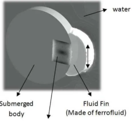
The aim of the present study is to numerically demonstrate the feasibility of using a smart fluid, specifically a ferrofluid as a small propulsive appendage resembling a fish tail or fin. The main idea is better illustrated in Fig. 2.

Fig. 2. Schematic of a fluid fin.

As observed in Fig. 2, magnetic actuators are located inside a submerged body and control the ferrofluid located outside the body. The ferrofluid is shaped in a way to form a fin-shaped structure. Subsequently, an oscillatory motion is induced to the fluid fin to make propulsion force.

By showing the feasibility of a fluid fin as a propulsion system, the authors have tried to show the possibility of using fluids in a wider range of applications. As a consequence of this study, one may imagine the replacement of solid materials with fluids in devices where rigid and solid parts limit the performance of the device. Fluid structures may include “fluid rudders”, “fluid walls and reservoirs”, “fluid propellers” and even “fluid skin” for “shape changing devices”. Also, by using electrically conducting ferrofluids, it is even possible to design fluid as shapeable and changeable electrical circuits, perhaps resulting in “flutronics” as a new concept in mechatronics. In the next section, the governing equations which are numerically solved by Ansys-CFX software are presented. Afterwards, the software’s ability to simulate the ferrohydrodynamic is assessed by modeling the stable state of a ferrofluid around a vertical electric current. Then, the main investigation is presented in the two above mentioned parts.

2. G

E

In this numerical study, the indtended simulations are conducted using the Ansys-CFX solver. The governing equations used in the numerical solver are briefly presented in this section (Ansys, 2015). The continuity of mass and momentum are as follows:

 

∇ ∂ ∂

=

ρU + t

ρ

(1)





t ρU

emag

 

 ∇ ∇

∇ ∂ ∂

(2)

where U is the fluid velocity vector and t, p, and ρ

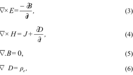
complexity of the problem is attributed to the use of Maxwell equations as in

, t

B = E ×

∂ ∂

∇  (3)

, t D + J = H ×

∂ ∂

∇ (4)

0,

∇

.B

=

, ρ =

D e

∇ (6)

to calculate Femag. In Eq. (3) through (6),

parameters B, D, E, H, J and ρe are magnetic

induction, electric displacement, electric field, magnetic field, current density, and electric charge density, respectively. Using these equations, the equation

H. M

μ

=

F_{emag 0} ∇ (7)

is extracted for Femag. In Eq. (7), M is the fluid

magnetization, H is the magnetic field and is the

magnetic permeability of the vacuum. The above momentum source assumes that free surface is stable. In other words, the surrounding fluid, the ferrofluid, and the magnetic field are set in a way that no instability occurs on the free surface. The differences between stable and instable free surfaces are displayed in Fig. 3.

Fig. 3. Stable and instable free surface in ferrofluids.

The focus of the present study is on the stable free surface, where no spikes occur. The Finite Volume method is used by Ansys-CFX to solve the presented governing equations for the ferrohydrodynamics problems. After this brief presentation of the governing equations, the validation of the ferrohydrodynamics software is presented in the following section.

3. V

In order to validate the numerical solver, the ascension of ferrofluids along a vertical electrical current carrying rod is modeled and results are compared against analytical solutions (Rosenweig, 1982).

To better describe the problem, a magnetic field is created around any rod carrying electrical current. The magnetic field attracts the ferrofluid which ascends along the rod and reaches an equilibrium state due to gravitational force.

Fig. 4. Response of a magnetic fluid to the steady electric current passing through a vertical rod

(Rosenweig, 1982).

Figure 4 illustrates an experimental result of the problem. The analytical solution of the stable elevation of the ferrofluid is presented by (Rosenweig, 1982).

2 2

2 0

8

π

ρ

gR

χ

I

μ

=

h

In Eq. (8), Δh is the elevation of the ferrofluid,

μ

is the magnetic permeability of the vaccum,

χ

the fluid magnetic sensitivity, I is the electric

current, while

ρ

density, gravitational acceleration, and the rod radius, respectively.

The setup of the problem is displayed in Fig. 5.

Fig. 5. Modeling of the validation problem.

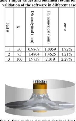
In the present simulation, the current is assumed to be 3.5 A, the rod radius is set to be 1mm, the

ferrofluid density is 997 kg/m3_{, and the magnetic}

sensitivity is varied as presented in Table 1 along with the obtained results for each case.

Table 1 Input values and obtained results for the validation of the software in different cases

Test #

X

Dh analy

tic

al

(m

m)

Dh numeri

cal

(

mm)

error

1 50 0.9869 1.0059 1.92%

2 75 1.4804 1.4625 1.21%

3 100 1.9739 2.019 2.29%

Fig. 6. Free surface elevation obtained for test case 1.

4. R

A

D

As pointed out earlier, two magnetic actuators are placed in a submerged body to control the ferrofluid shape and oscillatory motion in the current study. To this end, a computational domain with appropriate boundary conditions is required. Figure 3 shows the domain and numerical setup of the targeted analyses. Also, the boundary conditions are presented in Table 2.

Fig. 7. Numerical domain and boundary conditions.

Table 2 Setup boundary conditions

Momentum BCs Magnetic BCs

Body No slip wall Normal field

Actuators - Normal field

Far field Opening Zero field

Symmetries Symmetry Normal Field

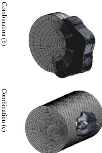
Also, three combinations of the magnetic actuators are assumed as shown in Fig. 8.

(a)

(b)

(c)

Fig. 8. Combination of magnetic actuators.

As observed in Fig. 8, the displayed combinations are essentially different to provide a better overview of the fluid fins produced in different combinations. In other words, in the present study, a preliminary study is conducted on the feasibility of the concept and not on the optimization of the system.

Combination (a) is a pseudo 2D analysis, where the fluid fin sides are not free. In other words, the magnetic actuators are extended to the side walls, preventing the water to flow freely around the fin. Combination (b) is involved with four actuators to show the flexibility of the fluid fin shaping with the magnetic field. As observed in both combinations of (a) and (b), the magnetic actuators are extended to the walls. However, in combination (c), the sides of the ferrofluid are free, i.e. both actuators are in the middle of the body and at a distance from the walls, allowing the water to flow around the ferrofluid.

4.1 Shaping Stage: the Initial Shape of the

Fluid Fin

To obtain the initial stable shape of the fluid fin, the magnetic actuators are activated and during a transient analysis, the actuators are left to shape the ferrofluid. In this process, which is the shaping stage of the fluid fin, the actuators are generating a steady magnetic field of 0.125 Tesla. The development process of the stable shaping of the ferrofluid in combination (a) is displayed in Fig. 9.

Initial condit

ion

t = 0.003

s

t = 0.005

s

t = 0.01

s

t = 0.03

s

(S

tabl

e s

h

ap

e)

Fig. 9. Shaping stage of the combination (a).

As observed in Fig. 9, the fluid quickly reaches its stable shape, a process which lasts under 0.07s for all considered combinations.

Also, the initial stable shapes obtained for combinations (b) and (c) are shown in Fig 10.

Combination (b)

Combination (c)

Fig. 10. Initial stable shapes obtained for combinations (b) and (c).

It should be pointed out that in combination (b), the outer magnetic actuators applies one tenth of the magnetic field of the middle ones, allowing the form shown in Fig. 10.

As observed above, after the shaping stage, different shapes of fins can be obtained. This is due to the fact that the ferrofluid free surface is shaped by the magnetic field. By comparing the initial stable shapes through the magnetic field isosurfaces for different combinations (Fig. 11), it is observed that the fluid fin tends to duplicate the magnetic field isosurfaces.

Fluid Fin Magnetic Field

Combination (a)

Combination (b)

Combination (c)

Fig. 11. Comparison of isosurfaces of the magnetic field and related fluid fin in different

Therefore, through designing the magnetic field isosurface shapes, the form of the fluid fin can be accurately predicted and designed.

So far, it is shown that the external shape of ferrofluids can be designed through altering the magnetic field. In addition, the very fast response of the fluid to the magnetic field (under 0.07s) shows the ability of using ferrofluids in devices where fast shape changing is required. This is a promising result for the “fluid structures” concept.

As observed, the ferrofluid is now placed on the submerged body as an external appendage which could play the role of a control surface as well as a lift surface. By inducing specific motions to the fluid fin, hydrodynamic forces can be produced.

4.2 Actuation Stage: Motion of the Fluid

Fin

After finding the stable shape of the fluid fin, an oscillatory magnetic field with a frequency of 40 Hz is applied to the fluid by the magnetic actuators. Because of the similarity of the actuation stage for all combinations, this process is only described for the combination (a). The magnetic field of the two actuators in combination (a) versus time is presented in Fig. 12.

0 0.05 0.1 0.15 0.2 0.25 0.3

0 0.05 0.1 0.15 0.2 0.25

M ag n et ic F ie ld ( T )

time (s)

Actuator 1

Actuator 2

Fig. 12. Magnetic field of the actuators Vs time.

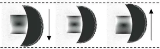
By applying the mentioned magnetic field to the ferrofluid, the overlapping magnetic field of the actuators results in a magnetic field which is transferred from an actuator to another. This changing magnetic field causes the ferrofluid to be transferred from one actuator to the other and oscillate. The motion of the fluid fin is illustrated in Fig. 13.

Fig. 13. Magnetic fluid motion with the magnetic field actuation (combination (a)) and the motion

direction of the fluid fin.

As observed in Fig. 13, the actuation of the magnetic field results in the oscillation of the ferrofluids in a course which eventually can be defined by the placement, power, and frequency of the actuators.

The pressure field change is illustrated (after 40

periods of magnetic field oscillation) in Fig. 14.

Fig. 14. Water pressure with motion of the magnetic fluid (combination (a)) and the

motion direction of the fluid fin.

As observed in Fig. 14, when the fin ascends, the water pressure increases above and decreases bellow the body, up to 15 Pa. The inverse occurs, when the fluid fin descends. It is expected that the fluid velocity also changes with the pressure. The velocity field is presented in Fig. 15 for the extreme conditions of the fin oscillation.

As expected, the fluid fin acts on the water as a solid fin and velocities up to 0.25 m/s are induced to the water from the fin. It should be pointed out that in some areas near the fin, the velocity increases up to 0.9 m/s which is a very high velocity produced by a 5 mm fin. Same results with slight differences can be found for other combinations.

As observed in Fig. 15, the actuation stage makes the fluid fin act like a pseudo solid fin and to affect the velocity and pressure field around the body. The obtained results show that not only the shape of the ferrofluid is fully controllable, but also the fluid shows enough rigidity to affect the surrounding fluid and induce pressure and velocity changes, all controllable via the magnetic actuators. This result extends the use of the “fluid structures” concept to a wider range of applications.

Fig. 15. Fluid velocity with motion of the magnetic fluid (combination (a)) and the motion

direction of the fluid fin.

4.3 Fluid Fin Thrust

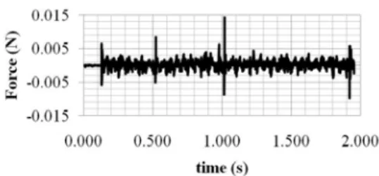
The propulsion forces acting on the fluid fin in different combinations are illustrated in Fig. 16.

Fig. 16. Thrust produced by the fluid fin versus time in different combinations.

As expected and observed in Fig. 16, the shaping stage of different combinations have different durations. Also, the magnitude of the thrust produced by the three combinations is different. The combination (a) produces the highest thrust, followed by the combination (c) and (b) in descending order. As observed in Fig. 16, it is also shown that, in the first part of the simulation related to the shaping stage, no significant force is generated.

However, as observed in Fig. 17, as soon as the magnetic field oscillation starts, the oscillating forces are produced on the fin.

Another interesting chart is the lateral force acting on the fluid fin. As an example and to have a clear view, the lateral force of combination (a) is displayed in Fig. 17.

Fig. 17. Thrust in the shaping stage (reaching a stable fluid fin shape).

Fig. 18. Lateral force produced by the fluid fin versus time.

As expected and observed in Fig. 18, the lateral force oscillates around 0 N. a relatively similar behavior happens in other combinations. After almost 30 periods, the forces become periodically steady for all cases. Figure 19 illustrates the forces on the fluid fin.

Fig. 19. Thrust produced by the fluid fin in propulsion stage for different combinations.

As shown in Fig. 18, the fluid fin produces an average thrust of 0.0158 N in combination (a) which is a large value relative to the size of the body. Also, for combinations (b) and (c), an average thrust of 0.0028 N and 0.00733 N are respectively obtained.

The main reason behind the low thrust of combination (c) is the fact that the water is free to flow around the ferrofluid; hence, a pressure release occurs and the thrust diminishes.

Fig. 20. The restriction of the ferrofluid motion in combination (b) and the motion direction of

the fluid fin.

As observed in Fig. 20, when the ferrofluid is expected to move upward and downward, the restriction causes it to have a lateral periodic motion inward and outward, which highly diminishes the produced thrust force.

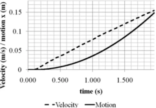
Regarding the results of the combination (a) and assuming that the submerged body weighs 0.2 kg, by integrating the force diagram (Fig. 16), the velocity and displacement of the body during this time could be roughly predicted. The velocity and displacement of the body during from the shaping stage to the actuation stage are illustrated in Fig. 2.1.

Fig. 21. Velocity and displacement of the submerged object via integration of thrust (Fig.

16) over time.

As observed in Fig. 21, the 1cm body weighting 0.2kg is displaced more than 0.15 cm with this amount of force. Thus, a structure made of fluid is designed which can be used as a propulsive appendage for the submerged bodies. Encouraged by the presented results, the authors have planed an experimental study on the fluid fins and also, the design of other applications of the fluid structures concept including fluid rudders, fluid propellers, shapeable streamlined high efficiency vessels, and fluid electrical circuits.

5.

C

In the present study, the feasibility of using a magnetic fluid to form a magnetically controllable and shapeable hydrodynamic propulsive fin for a submerged body is investigated. After reviewing the literature of the mathematical simulation of magnetic fluids and their applications, the concept of “Fluid Structures” and “Fluid Fin” is briefly

introduced. Afterward, a validation on the

capability of the numerical solver in analyzing the magnetic fluids is conducted against analytical solutions and acceptable errors of 1.21% up to 2.29% are reported.

For a better understanding of the performance of the fluid flap or fin in different designs, three different combinations of magnetic actuators are selected. Subsequently, the simulation of the fluid fin is conducted in two stages; the shaping stage and the actuation stage. In the shaping stage, the shaping process of the magnetic fluid on the outside surface of the submerged body, using internal magnetic actuators, is simulated and the initial stable shape of the fluid fin is presented. It is shown that the shape of the fluid fin is almost identical to the shape of magnetic field isosurface, which implies that through designing the magnetic field, the shape of the fluid fin can be exactly controlled. In the actuation stage, concerning the periodic oscillation of the fin, the magnetic actuators are forced to produce an oscillating magnetic field of a 40Hz frequency. It is demonstrated that the oscillating magnetic field makes the ferrofluid oscillate with the same frequency, producing pressure and velocity changes in the surrounding fluid and thus the propulsion force. The estimated average force generated by the fluid fin is up to 0.0158 N in one of the combinations. It is also shown that this amount of force is significant relative to the size of the body and the fin. Finally, it is concluded that a structure made of a shapeable fluid can be used as a fluid appendage for a submerged body.

R

Afkhami, S., Y. Renardy, M. Renardy, J. S. Riffle and T. St Pierre (2008). Field-induced motion of ferrofluid droplets through immiscible viscous media. Journal of Fluid Mechanics 610, 363-380.

Cowley, M. D. and R. E. Rosensweig (1967). The interfacial stability of a ferromagnetic fluid. Journal of Fluid mechanics 30(04), 671-688.

Frey, M. (2004). Snoil-A Physical Display Based

on Ferrofluid., http://www.freymartin.de/en/projects/snoil,

accessed on 2016.

Hartshorne, H., C. J. Backhouse and W. E. Lee (2004). Ferrofluid-based microchip pump and

valve. Sensors and Actuators B: Chemical

99(2), 592-600.

Khan, W. A., Z. H. Khan and R. U. Haq (2015). Flow and heat transfer of ferrofluids over a flat plate with uniform heat flux. The European Physical journal plus 130(4), 1-10.

Kodama, S. (2008). Dynamic ferrofluid sculpture: organic shape-changing art forms. Communications of the ACM 51(6), 79-81.

Koelman, Z., M. J. de Graaf and H. J. Lee (2015). From meaning to liquid matters. In Proceedings of the 21st International Symposium on Electronic Art.

Koh, J. T. K. V., K. Karunanayaka, J. Sepulveda, M. J. Tharakan, M. Krishnan and A. D. Cheok (2011). Liquid interface: a malleable, transient, direct-touch interface. Computers in Entertainment (CIE) 9(2), 7.

Laird, P. R., R. Bergamasco, V. Bérubé, E. F. Borra, J. Gingras and A. M. R. Ritcey (2003), Ferrofluid-based deformable mirrors: a new approach to adaptive optics using liquid mirrors, Astronomical Telescopes and

Instrumentation, International Society for

Optics and Photonics, 733-740.

Lajvardi, M., J. Moghimi-Rad, I. Hadi, A. Gavili, T. D. Isfahani, F. Zabihi and J. Sabbaghzadeh (2010). Experimental investigation for enhanced ferrofluid heat transfer under magnetic field effect. Journal of Magnetism and Magnetic Materials 322(21), 3508-3513.

Lavrova, O. (2006). Numerical methods for axisymmetric equilibrium magnetic-fluid shapes Ph. D. thesis, Otto-von-Guericke-Universität Magdeburg, Universitätsbibliothek.

Link, D. R., E. Grasland‐Mongrain, A. Duri, F. Sarrazin, Z. Cheng, G. Cristobal, ... and D. A. Weitz (2006). Electric control of droplets in microfluidic devices. Angewandte Chemie International Edition 45(16), 2556-2560.

Long, Z., A. M. Shetty, M. J. Solomon and R. G. Larson (2009). Fundamentals of magnet-actuated droplet manipulation on an open hydrophobic surface. Lab on a Chip 9(11), 1567-1575.

Malekzadeh, A., A. R. Pouranfard, N. Hatami, A.

K. Banari and M. R. Rahimi (2016). Experimental investigations on the viscosity of magnetic nanofluids under the influence of temperature, volume fractions of nanoparticles

and external magnetic field.Journal of Applied

Fluid Mechanics 9(2), 693-697.

Nguyen, N. T., K. M. Ng and X. Huang (2006). Manipulation of ferrofluid droplets using planar coils. Applied Physics Letters 89(5).

Prakash, J. (2014). On exchange of stabilities in ferromagnetic convection in a rotating ferrofluid saturated porous layer. Journal of Applied Fluid Mechanics 7(1), 147-154.

Rabbi, K. M., S. Saha, S. Mojumder, M. M. Rahman, R. Saidur and T. A. Ibrahim (2016). Numerical investigation of pure mixed convection in a ferrofluid-filled lid-driven cavity for different heater configurations. Alexandria Engineering Journal 55(1), 127-139.

Resler, E. L. and R. E. Rosensweig (1964). Magnetocaloric power. AIAA Journal 2(8), 1418-1422.

Rosensweig, R. E. (1982). Magnetic fluids. Scientific American 247(4), 136-145.

Rosensweig, R. E. (2013). Ferrohydrodynamics. Courier Corporation.

Sheikholeslami, M. and M. M. Rashidi (2015). Ferrofluid heat transfer treatment in the presence of variable magnetic field. The European Physical Journal Plus 130(6), 1-12.

Shliomis, M. I. (1968). Equations of motions of a fluid with hydromagnetic properties. Soviet physics JETP 26, 665.

Shliomis, M. I. (2001a). Ferrohydrodynamics: Testing a new magnetization equation. Physical Review E 64(6).

Shliomis, M. I. (2001b). Comment on Magnetoviscosity and relaxation in ferrofluids. Physical Review E 64(6).

Shliomis, M. I., T. P. Lyubimova and D. V. Lyubimov (1988). Ferrohydrodynamics: An essay on the progress of ideas. Chemical Engineering Communications 67(1), 275-290.

Shliomis, M. and Y. L. Raikher (1980). Experimental investigations of magnetic fluids. Magnetics, IEEE Transactions on 16(2), 237-250.

Yellen, B. B., G. Fridman, and G. Friedman (2004). Ferrofluid lithography. Nanotechnology 15(10). Zahn, M. (2001). Magnetic fluid and nanoparticle