Variable Temperature ⁵⁷Fe-Mössbauer Spectroscopy Study of Nanoparticle Iron Carbides

DOI: 10.5562/cca2782

Variable Temperature

57

_{Fe-Mössbauer Spectroscopy}

Study of Nanoparticle Iron Carbides

1 _{Materials and Engineering Research Institute, Sheffield Hallam University, City Campus, Howard Street, Sheffield, S1 1WB, UK} 2 _{Ecole des Mines de Nantes, 4 Rue Alfred Kastler, BP 20722, 44307 Nantes Cedex 3, France}

3 _{Johnson Matthey Technology Centre, Sonning Common, Reading, West Berkshire, RG4 9NH, UK} * Corresponding author’s e-mail address: Alex.Scrimshire@student.shu.ac.uk

RECEIVED: March 15, 2015  _{REVISED: July 15, 2015}  _{ACCEPTED: September 15, 2015}

THIS PAPER IS DEDICATED TO DR.SVETOZAR MUSIĆ ON THE OCCASION OF HIS 70TH _BIRTHDAY

Abstract: Near-phase-pure nanoparticle iron carbides (Fe3C and Fe5C2) were synthesised. Debye model calculations were used with hyperfine parameters gathered by 57_{Fe Mössbauer spectroscopy within a temperature range of 10 K to 293 K, with analysis providing Debye temperatures} of 422 K and 364 K for two Fe sites in Fe5C2 and 355 K for ferromagnetic Fe3C. The intrinsic isomer shifts were calculated as 0.45 mm s−1 _and 0.43 mm s−1 _{for iron sites 1 and 2 respectively in Fe5C2 and 0.42 mm s}−1 _{for Fe3C. Recoil-free fractions for the two iron sites were also calculated} at f300 0.785 and 0.726 for site 1 and 2 respectively.

Keywords: Mössbauer, iron carbides, Debye, Hägg, cementite, catalyst.

INTRODUCTION

RON carbides have a variety of uses and fields of interest, from their ubiquity in iron and steel manufacturing[1] _{to super capacitor electrodes}[2] _and

functionalized carbon nanotubes.[3] _{Iron-based catalysts}

are widely used in Fischer-Tropsch synthesis (FTS)[4,5] _with

iron carbides giving high levels of activity and selectivity in producing the desired longer hydrocarbon chains.[6]

Characteristics of iron carbides as compounds may vary greatly, as summarized in Table 1.

At present it is believed that the Hägg carbide (χ-Fe5C2 as in Table 1) is a highly active iron carbide phase in

FTS while cementite, Fe3C (also called Cohenite), is

considered far less active.[4,7] _{This work is intended to probe}

the iron environments within nanoparticle cementite and Hägg carbide as inactive and active FTS catalyst iron carbide phases in order to improve the understanding of these potential industrial catalysts. Through an increased understanding, and use of the Debye model to ascertain a Debye temperature for these phases, mixed-phase catalysts that have been in service may be studied to

determine any differences in phase abundance to relate their abundance to catalytic activity. Hence the aim is to more confidently identify active FTS iron carbide phases. Nanoparticles are being studied for their greater surface area by weight with the intent to identify any surface phases that would be in direct contact with the reactants. For these phases in low abundances, 57_{Fe transmission}

Mössbauer spectroscopy is the ideal technique to study these iron-rich materials. 57_{Fe Mössbauer spectroscopy}

uses gamma radiation emitted from a 57_{Co source to probe}

the 57_{Fe nuclei of a sample material, with an energy}

resolution to the order of 1 in 1012_,[8] _{allowing hyperfine}

Croat. Chem. Acta2015, 88(4), 531–537 DOI: 10.5562/cca2782 confident phase identification of mixed phase systems,

such as catalysts. This will allow comprehensive aging studies to be carried out, and active phases of a catalyst may be more confidently determined.

METHODOLOGIES

Two near-phase pure sample were synthesised, one of cementite (Fe3C) and one of Hägg carbide (Fe5C2). The

cementite was prepared by decomposition of a mixture of iron(III) acetate and gelatin at 700 °C.[9] _{The nanoparticles}

of Hägg carbide, Fe5C2, were prepared by decomposition of

iron pentacarbonyl in the presence of hexadecyltri-methylammonium bromide (CTAB) at 350 °C.[10] _{The details}

of the synthesis procedures may be found in the relevant sources provided.

X-ray diffraction was performed on a Bruker AXS D8 with a copper Kα source tube; 2θ 10 to 130; step size 0.022°; step time 176 seconds; 25 °C. Analysis of the samples indicated that the cementite samples contained 98 % Fe3C (04-003-6492) and 2 % Fe metal, and the Fe5C2

(00-036-1248) after synthesis indicated largely Fe5C2 with

traces of cementite and an undefined glassy phase indicated by a broad and tall peak with no defining features. After approximately 20 hours in air, XRD of the Fe5C2

sample clearly showed Fe5C2, trace amounts of cementite

and a potential indication of an iron oxide phase (00-046-1436).

57_{Fe Mössbauer spectroscopy, with a} 57_{Co in Rh}

source, was conducted on these samples between 293 and 10 K at a velocity range of ± 12 mm s−1 _{using a See Co W304}

and W202 drive unit and 1024 channel spectrometer, with a Janis CCS-800/204N cryostat and Lakeshore 335 tempe-rature controller. Each sample was diluted with fine powder graphite in order to achieve an ideal Mössbauer thickness in the absorber. Data collections above 100 K were conducted under vacuum. For data collections at or below 100 K, the cryostat chamber was filled with helium and maintained at ambient pressure with decreasing temperature. This helium was introduced as an exchange gas having found that temperatures below 100 K were

more difficult to maintain under a vacuum, while under helium temperatures of 10 K were easily held. The beginning of each collection was delayed by an hour once the temperature controller stated the desired temperature had been met to ensure the entire chamber was at temperature and to ensure temperature stability.

RESULTS

Each synthesis produced very fine, black, magnetic nanoparticles with XRD identification indicating near phase pure materials. The expected room temperature Mössbauer hyperfine parameters from literature in Tables 2 and 3 present data for nanoparticles and bulk Fe5C2

respectively. Uncertainties were not given and where these sources have stated isomer shift, this is most likely meaning centre shift, however this has been kept as IS.

Experimental values gathered during this study for Fe5C2 for the sites most consistent with literature values are

presented in Tables 4 and 5 over the temperature range 10 to 293 K. All Mössbauer data from this work is relative to α-Fe calibration.

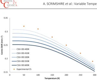
Figures 1 and 2 show the relation between the experimental values for centre shifts across the temperature range and the expected trends for Debye temperatures of 400 to 600 K, for the two iron sites presented in Tables 4 and 5. As seen in Figure 1, the 100 K data is not consistent with the other experimental centre Table 1. Iron carbide phase characteristics[6]

Atomic ratio Interstitial occupation Wt%

Formula (C : Fe) Crystal lattice of carbon atoms C

Hexagonal carbide ε Fe₂C 0.5 hcp to monoclinic Octahedral 9.7

ε' Fe₂.₂ 0.45 hcp to monoclinic Octahedral 8.9

Eckstrom and Adcock carbide Fe7C3 0.43 Orthorhombic Trigonal prismatic 8.4

Hägg carbide χ Fe5C2 0.4 Monoclinic Trigonal prismatic 7.9

Cementite θ Fe3C 0.33 Orthorhombic Trigonal prismatic 6.7

FexC

Table 2. Nanoparticle Fe5C2 Mössbauer parameters[11]

Iron Site IS / mm s–1 _{H / T ε / mm s}–1

Site 1 0.288 21.5 0.055

Site 2 0.171 18.16 –0.049

Table 3. Bulk sample Fe5C2 Mössbauer parameters[6]

Iron Site IS / mm s–1 _{H / KoE [T]}

Site 1 0.46 189 [18.9]

Site 2 0.51 218 [21.8]

DOI: 10.5562/cca2782 Croat. Chem. Acta2015, 88(4), 531–537 shift trend, and as such it was omitted from calculations to

come.

Figure 3 shows the Mössbauer spectra for 293, 150 and 137.5 K, chosen for the visible additional phase becoming present at 137.5 K at around the ± 8 mm s−1

regions. Mössbauer spectra were fitted using Lorentzian model lines with Recoil software. The fitting process allowed centre shift, magnetic splitting, quadrupole shift area and linewidth to vary, while the sextets were

constrained to a 3:2:1 ratio regarding the peak height, and the linewidth of paired peaks (1 and 6, 2 and 5, 3 and 4) were kept the same.

Tables 6 and 7 present existing literature data for Fe3C, all concerning room temperature measurements,

uncertainties were not provided by the authors, nor was the calibration material stated; it is assumed to be α-Fe.

There is also reportedly a doublet associated with Fe3C at 293 K. Table 7 contains the experimental data

Table 4. Experimental values of Mössbauer hyperfine parameters for site 1; nanoparticles of Fe5C2. CS: Centre shift (± 0.02 mm s–1);

H: Magnetic splitting (± 0.5 T); Γ/2 = HWHM (± 0.02 mm s–1_{); ε: Quadrupole shift (± 0.02 mm s}–1₎

T / K CS / mm s–1 _{H / T (Γ/2) / mm s}–1 _{ε / mm s}–1

293 0.23 21.9 0.19 0.03

250 0.24 22.4 0.18 0.04

200 0.27 23.3 0.18 0.03

150 0.30 24.2 0.18 0.03

147.5 0.30 24.2 0.17 0.03

137.5 0.31 24.3 0.17 0.03

125 0.31 24.5 0.17 0.03

100 0.32 24.6 0.22 0.02

50 0.33 25.2 0.18 0.02

10 0.34 25.4 0.17 0.03

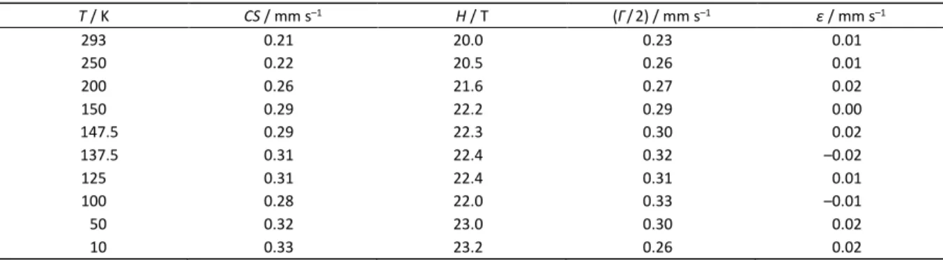
Table 5. Experimental values of Mössbauer hyperfine parameters for site 2; nanoparticles of Fe5C2. CS: Centre shift (± 0.02

mm s–1_{); H: Magnetic splitting (± 0.5 T); Γ/2 = HWHM (± 0.02 mm s}–1_{); ε: Quadrupole shift (± 0.02 mm s}–1₎

T / K CS / mm s–1 _{H / T (Γ/2) / mm s}–1 _{ε / mm s}–1

293 0.21 20.0 0.23 0.01

250 0.22 20.5 0.26 0.01

200 0.26 21.6 0.27 0.02

150 0.29 22.2 0.29 0.00

147.5 0.29 22.3 0.30 0.02

137.5 0.31 22.4 0.32 –0.02

125 0.31 22.4 0.31 0.01

100 0.28 22.0 0.33 –0.01

50 0.32 23.0 0.30 0.02

10 0.33 23.2 0.26 0.02

Figure 1. Experimental centre shifts of Fe5C2 site 1 against

theoretical centre shift trend lines calculated.

Figure 2. Experimental centre shifts of Fe5C2 site 2 against

Croat. Chem. Acta2015, 88(4), 531–537 DOI: 10.5562/cca2782 gathered in this work for the corresponding sextet, over a

temperature range of 50 to 293 K.

Figure 4 shows the experimental centre shifts with temperature, and the expected trends according to the

Debye model. All data points appear to follow the expected trend within the Debye model, and as such all were included and used in further calculations.

ANALYSIS AND DISCUSSION

The room temperature hyperfine parameters from literature (Tables 2 and 3) are notwithin the experimental uncertainties for the current experimental values for the two iron sites of Fe5C2 in Tables 4 and 5. While the spectrum

of Fe5C2 at roomtemperature does have more components

than the two sextets presented in Cheng,[11] _{their synthesis}

route is different to that used for this study, and material synthesisroute is believed to have an effect on hyperfine structure and therefore on the Mössbauer data.[13] _The

trend seen for both iron sites agree with that expected for the Debye model, as seen in Figures 1 and 2. Within the Debye Model framework,[14] _{the recoil free fraction}

parameter can be determined by equation 1:

2 Θ 2

2

0

3 1 1 d

ln

4 1

D T

γ

x

D D

E T x x

f

Mc kΘ Θ e

 _{ } 

 

     _

   





where (in case of 57_{Fe-Mössbauer study):}

Eγ, Energy of the gamma ray = 14.4125 keV (2.30914 × 10–15 _J), M, Mass of 57_{Fe = 9.46507 × 10}–26 _kg,

c, Speed of light = 299 792 458 m s–1_,

k, Boltzmann constant = 1.38065 × 10–23 _{J K} –1_,

ΘD, Debye temperature – Sample dependent constant (K),

T, Absolute temperature of the sample – Variable (K) Figure 3. Experimental data and Lorentzian line fits of Fe5C2

Mössbauer spectra.

Table 6. Nanoparticle ferromagnetic Fe3C Mössbauer

hyper-fine parameters[12]

T / K CS / mm s–1 _{H / T ε / mm s}–1

293 0.19 20.5 0.01

60 0.32 24.9 –0.05

27 0.32 25.0 0.01

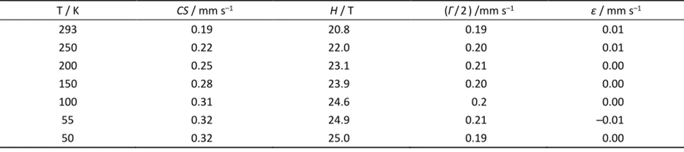
Table 7. Experimental Mössbauer Parameters of Fe3C, CS Relative to α-Iron. CS: Centre shift (± 0.02 mm s−1); H: Magnetic

splitting (+/- 0.5 T); Γ/2 = HWHM (± 0.02 mm s–1_{); ε: Quadrupole shift (± 0.02 mm s}−1₎

T / K CS / mm s–1 _{H / T (Γ/2) /mm s}–1 _{ε / mm s}–1

293 0.19 20.8 0.19 0.01

250 0.22 22.0 0.20 0.01

200 0.25 23.1 0.21 0.00

150 0.28 23.9 0.20 0.00

100 0.31 24.6 0.2 0.00

55 0.32 24.9 0.21 –0.01

DOI: 10.5562/cca2782 Croat. Chem. Acta2015, 88(4), 531–537 The Debye Temperature ΘDis required to find the

recoil free fraction f.

Equation 2 shows the Second Order Doppler effect (SOD) as a function of the Temperature Tand the Debye temperature ΘD:





0

3 3 ₃ d

2 8 1

D T

D

x D

kΘ T x x

SOD m s

Mc Θ e

 _{ } 

 

     _

   





Equation 3 links the Second Order Doppler effect (SOD) to the Centre Shift(CS):

T Θ, D T Θ, D

CS IS SOD (3)

where IS, the Isomer Shift, which is considered to be independent of the temperature. By setting these equations as spreadsheet functions the Debye temperature can be calculated. At a given temperature the spreadsheet solver function will vary the Debye Temperature ΘD and the

isomer shift, calculate a theoretical centre shift CSth by means of equations 2 and 3 and compare it with the experimental one CSexp. Let:





Δ Θ IS TD, ,  CS _D IS T CS T (4)

Function 4 shows the absolute value of the difference between the theoretical value of centre shift (at given Debye Temperature, isomer shift and temperature) and the experimental one (at given temperature).

By varying the Debye Temperature ΘD and the

isomer shift step by step, the solver will try to minimize the sum Σ(ΘD, IS) of deltas Δ(ΘD, IS, T) corresponding to all the

temperatures experimentally analysed:













Σ Θ ISD, Δ Θ ISD, , 293 K  ... Δ Θ ISD, ,10 K (5)

The Debye Temperature and isomer shift being calculated can be set with constrictions, such that the initial calculation is run with wide allowances, before the values are constricted, with larger numbers of iterations with smaller allowable windows. Once Σ(ΘD, IS)is minimized, the

Debye Temperature ΘD and the isomer shift IS are known.

Then, it becomes possible to calculate the recoil free fraction f by means of equation 1. By manipulating these equations for set Debye Temperatures, the trend lines in Figures 1 and 2 were plotted for comparison with the experimental centre shifts gathered in this study, allowing Figure 4. Experimental centre shifts of Fe3C against

theoretical centre shift trend lines calculated.

Figure 5. Experimental data of Fe3C Mössbauer spectra with

Croat. Chem. Acta2015, 88(4), 531–537 DOI: 10.5562/cca2782 an estimate of the actual Debye temperature to be made

and used as a limiting parameter for the solver function. By utilising these Debye model equations with the experimental data gathered, the Debye Temperature of Fe5C2 iron site 1 was determined as 422 K, and site 2 as 364

K. The intrinsic isomer shifts were calculated as 0.45 mm s−1

and 0.43 mm s−1 _{(± 0.03 mm s}−1_{) for iron sites 1 and 2}

respectively. These were calculated by omitting the 100 K and 293 K data as these did not agree with the trends expected in the Debye model, the reason for this being currently unknown. Although experimental error may allow these values to have been used, with the current functions being used in the spreadsheet formula, it is necessary that decreases in temperatures is accompanied by increases in centre shift, or else the function is not satisfied and errors are returned. The sum of the magnitude of differences between the theoretical and experimental centre shifts as presented in equation 5 was 0.03 without the 100 K and 293 K data, which may be considered the uncertainty of the intrinsic isomer shifts stated.

The Fe3C data from Table 7 was also processed using

the Debye model calculation spreadsheet, yielding an intrinsic isomer shift of 0.42 mm s−1 _{(± 0.03 mm s}−1_{) and a}

Debye temperature of 355 K. The magnitude of the differences between the theoretical and experimental data was 0.03, which may again be considered the uncertainty. Data from Fe3C collected below 55 K was not included in

this work, due to the spectral change seen in the 50 K spectrum of Figure 5. The nature of this spectral change is not currently known, but can be seen in the 2009 work by David et al.[12]

For comparison of Debye temperatures, it appears that different methods of calculation, and the experimental approach used has profound effects on the outcome, as summarised in Table 8 for Fe3C.

As such, the values stated in this work are for consideration of Mössbauer data, and the mathematical approach using the Debye model as detailed. This wide range of existing values may be due to the nature in which the Fe3C is being studied, while that studied in this work is

ex situ as nanoparticles. A combination of the approaches used by each author, the particle size and surrounding matrix of the cementite may give rise to these great variances in reported values.

The difference between Debye temperatures of the two identified iron sites within Fe5C2 indicates that the iron

in site 1 is held more tightly than the iron in site 2. A higher Debye temperature gives a higher recoil-free fraction, and site 1 will contribute more to the Mössbauer spectrum than the same amount of iron in site 2. Through the execution of equation 1 within our program we can calculate the recoil free fractions for both site 1 and site 2 as f300 0.785 and 0.726, respectively. The greater recoil-free fraction would

agree with the greater Debye temperatures calculated for the two iron sites in Fe5C2, both caused by site 1 being more

tightly bound and therefore less able to vibrate than iron site 2.

The hyperfine parameters gathered through this study, and the Debye temperature and recoil-free fraction that can be calculated can be used to confidently identify mixed iron carbide materials, such as catalysts after having been in service, to enable aging studies. By having reference data to refer to for mixed phase samples, any phases that may evolve through catalytic activity can be identified to better understand the nature of the catalysis.

CONCLUSIONS

Through the use of Debye model equations, Debye temperatures for nanoparticle iron carbides were calculated using variable temperature 57_{Fe Mössbauer}

spectroscopy hyperfine parameter data. Intrinsic isomer shifts of Fe5C2 and Fe3C were proposed by using this

method, all of which may aid in better understanding these carbide phases, and mixed phase systems that contain one or both of those studied.

REFERENCES

[1] G. Marest, A. Fontes, J. Roigt, A. Faussemagne, S. Fayeulle, M. Jeandin, A. Benyagoub, N. Moncoffre, M. Frainais, Hyperfine Interact. 1995, 95, 227. [2] M. Yan, Y. Yao, J. Wen, W. Fu, L. Long, M. Wang, X.

Liao, G. Yin, Z. Huang, X. Chen, J. Alloy. Compd. 2015,

641, 170.

[3] Q. Su, G. Zhong, J. Li, G. Du, B. Xu, Appl. Phys. A-Mater. 2012, 106, 59.

[4] J. W. Niemantsverdriet, A. M. Van der Kraan, W. L. Van Dijk, H. S. Van der Baan, J. Phys. Chem. 1980, 84, 3363.

[5] G. Le Caer, J. M. Dubois, M. Pijolat, V. Perrichon, P. Bussiere, J. Phys. Chem. 1982, 86, 4799.

[6] E. de Smit, B. M. Weckhuysen, Chem. Soc. Rev. 2008,

37, 2758.

[7] V. P. Santos, T. A. Wezendonk, J. J. D. Jaén, A. I. Dugulan, M. A. Nasalevich, H.-U. Islam, A. Chojecki, Table 8. Summary of published Debye temperatures for Fe3C by author

Source Fe3C Debye Temperature

Reported (K)

This work 355 (± 25)

Ledbetter[15] _{501 (± 27)}

Wood[16] _{604 (± 44)}

DOI: 10.5562/cca2782 Croat. Chem. Acta2015, 88(4), 531–537 S. Sartipi, X. Sun, A. A. Hakeem, A. C. J. Koeken,

M. Ruitenbeek, T. Davidian, G. R. Meima, G. Sankar, F. Kapteijn, M. Makkee, J. Gascon, Nature Communications, 2015, 6, 6451.

[8] F. Berry, D. Dickson, Mössbauer Spectroscopy, Cam-bride University Press, 2005. ISBN 0-521-01810-2. [9] Z. Schnepp, S. C. Wimbush, M. Antonietti, C.

Giordano, Chem. Mater. 2010, 22, 5340.

[10] C. Yang, H. Zhao, Y. Hou, D. Ma, J. Am. Chem. Soc. 2012, 134, 15814.

[11] K. Cheng, M. Virginie, V. V. Ordomsky, C. Cordier, P. A. Chernavskii, M. I. Ivantsov, S. Paul, Y. Wang, A. Y.

Khodakov, J. Catal. 2015, 328, 139.

[12] B. David, O. Schneeweiss, F. Dumitrache, C. Fleaca, R. Alexandrescu, I. Morjan, J. Phys. Conf. Ser. 2010,

217, 012097.

[13] B. Hannoyer, A. A. M. Prince, M. Jean, R. S. Liu, G. X. Wang, Hyperfine Interact. 2006, 167, 767.

[14] J. J. Quinn, K.-S. Yi,Debye Model. Solid State Physics, Principles and Modern Applications, Springer, 2009. [15] H. Ledbetter, Mater. Sci. Eng. A, 2010, 527, 2657. [16] B. J. Wood, Earth Planet. Sci. Lett. 1993, 117, 593. [17] A. F. Guillermet, G. Grimvall, J. Phys. Chem. Solids,