Prescribed-burning vs. wildfire: management implications for annual carbon emissions along a latitudinal gradient of <i>Calluna vulgaris</i>-dominated vegetation

(1)

BGD

12, 17817–17849, 2015

Prescribed-burning vs. wildfire

V. M. Santana et al.

Title Page

Abstract Introduction

Conclusions References

Tables Figures

◭ ◮

Back Close

Full Screen / Esc

Printer-friendly Version Interactive Discussion

Discussion

P

a

per

|

Discussion

P

a

per

|

Discussion

P

a

per

|

Discussion

P

a

per

|

Biogeosciences Discuss., 12, 17817–17849, 2015 www.biogeosciences-discuss.net/12/17817/2015/ doi:10.5194/bgd-12-17817-2015

This discussion paper is/has been under review for the journal Biogeosciences (BG). Please refer to the corresponding final paper in BG if available.

Prescribed-burning vs. wildfire:

management implications for annual

carbon emissions along a latitudinal

gradient of

Calluna vulgaris

-dominated

vegetation

V. M. Santana1,2, J. G. Alday1, H. Lee3, K. A. Allen1, and R. H. Marrs1

1

School of Environmental Sciences, University of Liverpool, UK

2

Department of Environment and Planning, Centre for Environmental and Marine Studies (CESAM), University of Aveiro, Portugal

3

Eco-Safety Research Team, National Institute of Ecology, South Korea

Received: 11 September 2015 – Accepted: 27 October 2015 – Published: 9 November 2015 Correspondence to: V. M. Santana ([email protected])

(2)

BGD

12, 17817–17849, 2015

Title Page

Tables Figures

◭ ◮

Back Close

Full Screen / Esc

Discussion

P

a

per

|

Discussion

P

a

per

|

Discussion

P

a

per

|

Discussion

P

a

per

|

Abstract

A present challenge in fire ecology is to optimize management techniques so that ecological services are maximized and C emissions minimized. Here, we model the e_ffects of di_fferent prescribed-burning rotation intervals and wildfires on carbon emis-sions (present and future) in British moorlands. Biomass-accumulation curves from four

5

Calluna-dominated ecosystems along a north–south, climatic gradient in Great Britain were calculated and used within a matrix-model based on Markov Chains to calculate above-ground biomass-loads, and annual C losses under di_fferent prescribed-burning rotation intervals. Additionally, we assessed the interaction of these parameters with an increasing wildfire return interval. We observed that litter accumulation patterns varied

10

along the latitudinal gradient, with di_fferences between northern (colder and wetter) and southern sites (hotter and drier). The accumulation patterns of the living vege-tation dominated byCalluna were determined by site-specific conditions. The optimal prescribed-burning rotation interval for minimizing annual carbon losses also di_ffered between sites: the rotation interval for northern sites was between 30 and 50 years,

15

whereas for southern sites a hump-backed relationship was found with the optimal interval either between 8 to 10 years or between 30 to 50 years. Increasing wildfire fre-quency interacted with prescribed-burning rotation intervals by both increasing C emis-sions and modifying the optimum prescribed-burning interval for C minimum emission. This highlights the importance of studying site-specific biomass accumulation patterns

20

with respect to environmental conditions for identifying suitable fire-rotation intervals to minimize C losses.

1 Introduction

The capacity of controlling carbon (C) budgets at global and regional scales is a key step in tackling anthropogenically-driven climate change (Schimel and Baker, 2002).

25

(3)

BGD

12, 17817–17849, 2015

Title Page

Tables Figures

◭ ◮

Back Close

Full Screen / Esc

Discussion

P

a

per

|

Discussion

P

a

per

|

Discussion

P

a

per

|

Discussion

P

a

per

|

through biomass burning will determine whether a particular ecosystem is a net source or sink for C (Schimel et al., 2001; Pan et al., 2011). It is well known that at the global scale wildfires in fire-prone ecosystems release significant amounts of C annually (van der Werf et al., 2010). On the other hand, prescribed fire is also a significant C source, but it is commonly used as management tool for minimizing wildfire hazard, maintaining

5

habitat quality, creating new agricultural land and stimulating pasture and forest regen-eration (Harris et al., 2011; Bradstock et al., 2012; Bargann et al., 2014; Alday et al., 2015). An obvious, yet ambitious, challenge for ecologists is, therefore, to optimize prescribed fire management techniques to maximize provision of required ecological services and minimize C emissions (Bowman et al., 2009; Bradstock et al., 2012;

Fer-10

nandes et al., 2013). Whilst C emissions are a global problem, management solutions must be locally-based and dependent on the specific characteristics of each ecosys-tem (Galford et al., 2010; Post et al., 2012; Allen et al., 2013). The failure to develop regional management plans, holistically-coordinated with the aim of reducing C emis-sions and increasing C fixation will slow e_fforts for tackling climate change at the global

15

scale (Schimel and Baker, 2002; Bowman et al., 2009).

Undoubtedly, the potential of a given ecosystem to release C by combustion will be determined by the amount of available above-ground biomass – the fuel load (Allen et al., 2013; Collins et al., 2015). Where there are no constraints on plant productivity, for example fire or grazers, the above-ground biomass of terrestrial vegetation is

de-20

termined largely by climate (temperature and rainfall), but modified locally by soil-type, land management and historic land use (Bond and Keeley, 2005; Eriksson et al., 2002). Such climate-induced gradients of biomass production are clearly defined worldwide, and embrace scales ranging from local ecosystems to biomes (Holdridge, 1947; Bond and Keeley, 2005). Indeed, ecosystem properties that control biomass accumulation,

25

(4)

ac-BGD

12, 17817–17849, 2015

Title Page

Tables Figures

◭ ◮

Back Close

Full Screen / Esc

Discussion

P

a

per

|

Discussion

P

a

per

|

Discussion

P

a

per

|

Discussion

P

a

per

|

tivity at global- and regional-scales is linked to these climate-induced gradients (Pausas and Ribeiro, 2013), and it will provide evidence-based information to establish reliable policies for minimizing C losses along the gradients (Stewart et al., 2005).

Apart from the available biomass, fire regime and its fluctuations are important fac-tors controlling C emissions in any given ecosystem. The fire-return interval, for

ex-5

ample, defines the accumulated amount of biomass burned within a period of time, which is clearly a function of the ecosystem regeneration capacity through time (Allen et al., 2013; Alday et al., 2015). Similarly, fire severity (i.e. the amount of organic mat-ter consumed by fire) (Keeley, 2009) is also important in demat-termining the combustion completeness (CC) in a particular fire event. For example, differences in CC between

10

wildfires and prescribed fires should be expected, with greater amounts being lost un-der wildfire conditions. Normally, wildfires occur within fire-prone days (i.e., dry and hot conditions), and can produce the devastation of large areas and high CC; in some cases the fire can burn into the underlying soil organic layers, increasing the amounts of C lost (Maltby et al., 1990). In contrast, prescribed fires should be only performed

un-15

der controlled climatic conditions, so that undesirable escape fires are avoided, and CC should be much lower (Maltby et al., 1990; Allen et al., 2013). Determining the e_ffects of fire regime variations on C emissions is, therefore, fundamental to understanding C budgeting and to design appropriate management systems. Increasing our knowledge in this area is crucial because of global climate change; forecasts for the next few

20

decades predict shifts in wildfire regimes in many fire-prone ecosystems worldwide through increasing dry, hot summer climates with an obvious predicted increase in wildfire frequency, area burned and CC (Krawchuk et al., 2009).

Excellent examples of fire-prone ecosystems that are traditionally-managed by pre-scribed burning are moorlands and heathlands dominated by the dwarf shrubCalluna

25

(5)

BGD

12, 17817–17849, 2015

Title Page

Tables Figures

◭ ◮

Back Close

Full Screen / Esc

Discussion

P

a

per

|

Discussion

P

a

per

|

Discussion

P

a

per

|

Discussion

P

a

per

|

These moorlands are now also required to provide a range of ecosystem services rang-ing from biodiversity, the provision of potable water and C storage (Bain et al., 2011; Harris et al., 2011; Lee et al., 2013). Here, land managers periodically apply rotational prescribed burning during winter (October to mid-April) within a licensed framework (Anon, 2014; example for England). Specifically, prescribed should only be done when

5

climatic conditions are optimal for minimizing fire escapes and ecosystem damage. However, there has been increasing controversy in the last years about the optimal fire rotation interval (Bain et al., 2011; Lee et al., 2013). The current recommendations in England and Wales are that rotations should be no less than 10 years (Natural Eng-land, 2007), whereas in Scotland recommendations are to burn only heather taller than

10

20 cm (Scottish Government, 2011). The actual rotation interval, in contrast, is closer to 20 years in England (Yallop et al., 2006) and may be as much as 50–100 years in Scot-land (Hester and Sydes, 1992). In terms of C storage, there is no a clear management recommendation forCalluna-dominated ecosystems. Some practitioners suggest that prescribed burning should be halted altogether (Tucker, 2003). Allen et al. (2013), on

15

the other hand, recommended a rotation interval either of short duration (8–12 years) or long duration (>25 years) for a moorland in central England, but an avoidance of intermediate durations.

One of the major difficulties in defining generalised management prescriptions is the wide di_fferences in growth rates and biomass loads along climatic gradients within

20

Great Britain (Alday et al., 2015). Clearly, any rotation interval has a potential associ-ated annual carbon loss, which depends on the biomass accumulassoci-ated between burns and the fire-return interval. It is, therefore, important to develop site-specific manage-ment plans which reflect site biomass accumulation when developing methods for re-ducing C emissions. In this assessment, however, it is essential to take into account

25

(6)

BGD

12, 17817–17849, 2015

Title Page

Tables Figures

◭ ◮

Back Close

Full Screen / Esc

Discussion

P

a

per

|

Discussion

P

a

per

|

Discussion

P

a

per

|

Discussion

P

a

per

|

interval, C emissions from potential wildfire could be minimized. Further assessments of the interaction between prescribed burning rotation interval and wildfire using multi-ple contrasting sites are needed for predicting future emissions scenarios, especially as wildfire frequency is predicted to increase as a consequence of ongoing global climate change (Jenkins et al., 2009; Krawchuk et al., 2009; Albertson et al., 2011).

5

Here, we assess C emissions resulting from different prescribed-burning rotation intervals at sites with differing biomass patterns. We used biomass-load accumulation data from fourCalluna-dominated ecosystems along a north–south gradient in Great Britain. The matrix-model based on Markov Chains developed in Allen et al. (2013) was used to calculate under different prescribed-burning rotation intervals: (i) above-ground

10

biomass-loads, and (ii) annual C losses. Additionally, in order to assess the impact of future climate change scenarios we assessed the effects of (iii) increasing combustion completeness (CC) on its own, and (iv) interacting with a variable wildfire return interval (every 50, 100 and 200 years). Although no estimates of peat accumulation or loss are included in our models, the above-ground biomass load assessments are fundamental

15

to develop site-specific management plans for reducing C emissions. Specifically, here we tested the following hypotheses:

– Hypothesis 1: The biomass accumulation patterns of the main above-ground com-ponent fractions (i.e., litter andCalluna) will increase along the latitudinal gradient.

– Hypothesis 2: The optimal prescribed-burning rotation interval, (i.e., the point at

20

which annual C loss is minimized) will be controlled by the di_fferent site-induced patterns of biomass accumulation.

(7)

BGD

12, 17817–17849, 2015

Title Page

Tables Figures

◭ ◮

Back Close

Full Screen / Esc

Discussion

P

a

per

|

Discussion

P

a

per

|

Discussion

P

a

per

|

Discussion

P

a

per

|

2 Methods

2.1 Site descriptions

Biomass accumulation was measured in four contrasting moorlands/heathlands lo-cated on a north to south transect running through Great Britain (Fig. 1). Kerloch, the most northerly site, is in Kincardineshire, north-east Scotland (altitude range = 5

140–280 m). Two sites, Moor House and Howden, are located at opposite ends of the Pennines; the range of hills that form the backbone of England (Fig. 1). Moor House is at the northern end in Cumbria (altitude range=600–650 m), whereas How-den is at the southern end in the Peak District National Park, Derbyshire (altitude range ₌272–540 m). Finally, biomass data were available from three southern sites

10

(Hartland Moor, Studland Heath and Morden Bog) which are fairly close together in Dorset; all at low altitude (≤15 m).

In general, the climate is oceanic but there is a considerable gradient from north to south, also influenced by the altitude. Kerloch is the coldest site with an annual mean temperature of 7.3◦C, followed by Moor House (8.1◦C), Howden (9◦C), and Dorset, the

15

warmest site, with an annual mean temperature of 10.4◦C. Annual rainfall, however, does not follow the temperature pattern; Moor House experiences the highest pre-cipitation (1314 mm), followed by Kerloch (1040 mm), Howden (829 mm) and Dorset (800 mm). The four contrasting moorlands also di_ffered in soil types. The vegetation at both Moor House and Howden is on Blanket Bog (peat >50 cm); the underlying

20

bedrock at Moor House comprises a series of almost horizontal beds of limestone, sandstone and shale (Heal and Smith, 1978), whereas at Howden it is a mixture of mudstone, siltstone and sandstone (Rosenburgh et al., 2013). Both sites are dissected by gullies but none of them have been drained actively. Soils at Kerloch, in contrast, are poorly-drained, peaty podzols derived from granite and granitic gneiss (Miller, 1979),

25

(8)

BGD

12, 17817–17849, 2015

Title Page

Tables Figures

◭ ◮

Back Close

Full Screen / Esc

Discussion

P

a

per

|

Discussion

P

a

per

|

Discussion

P

a

per

|

Discussion

P

a

per

|

Heathlands and moorlands are managed in three ways across this latitudinal gra-dient: (1) two of the upland sites (Howden and Kerloch) were managed by rotational prescribed burning to increase sheep and/or red grouse production. Moor House has been managed actively in the past, but prescribed burning has not been carried out on this site since it became a National Nature Reserve in 1952, the exception being

5

a small-scale experiment designed to test di_fferent burning rotations (and used here). In Dorset, the vegetation management is totally different with the vegetation being al-lowed to go through theCallunafour-phase, growth-cycle defined by Watt (1947, 1955), although the cycle is interrupted frequently by wildfire. The Dorset data used here, de-scribes the vegetation regeneration after wildfire (see below), however, it may be used

10

as a proxy of a possible regeneration after intense prescribed burning.

The diverse climatic and management conditions combine to produce di_fferent plant communities, albeit all dominated byCalluna. The vegetation at Moor House and How-den can be described asCalluna vulgaris-Eriophorum vaginatumblanket mire (M19) and Eriophorum vaginatum blanket and raised mire (M20) communities within the

15

British National Vegetation Classification (NVC) (Rodwell, 1991). At the Kerloch site, the community was described as a Calluna vulgaris-Erica cinerea heath (H10) with possible small areas of Calluna vulgaris-Vaccinium myrtillus heath (H12). In Dorset, the species list was abstracted from Chapman (1967) and NVC classes fitted using the TABLEFIT program (Hill, 2011); the best fit (mean>66 %) community was theCalluna

20

vulgaris-Ulex minorheath (H2) community.

In spite of these between-site di_fferences, it was possible to collect space-for-time substitution data on changes in biomass (litter andCalluna) at each site, encompass-ing the main growth-phase-cycles ofCallunadevelopment. Data on biomass accumu-lation at Kerloch and Dorset was abstracted from previously-published literature

(Ker-25

(9)

BGD

12, 17817–17849, 2015

Title Page

Tables Figures

◭ ◮

Back Close

Full Screen / Esc

Discussion

P

a

per

|

Discussion

P

a

per

|

Discussion

P

a

per

|

Discussion

P

a

per

|

2.2 Biomass assessment: collection and derivation

Kerloch biomass was obtained from Miller (1979) where a space-for-time substitu-tion study allowed a reconstrucsubstitu-tion of biomass accumulasubstitu-tion over a 41 year period since burning. Six stands within a 1 km of each other were selected to form a se-ries of increasing age since burning (2, 8, 14, 18, 24 and 36 years). Every stand

5

was sampled annually for a period of six years. Additionally, two stands were specif-ically burnt and sampled to assess during the early stages of post-fire recovery. For our study, we took the mean values for each stand as presented graphically in Miller (1979) using the online tool provided by the German Astrophysical Virtual Observatory (http://dc.zah.uni-heidelberg.de/sdexter, accessed 16 January 2014).

10

Data for Moor House was described in Alday et al. (2015). The experiment was set up in 1954/5 with four replicate permanent blocks. All blocks were completely burned in 1954/5. Within each block, there were two main-plots to which two grazing treatments (sheep grazing and no sheep grazing) were allocated randomly. Then, within each main-plot, three burning-rotation treatments were also allocated randomly to sub-plots,

15

these were: (i) short-rotation burning (ca. every 10 years), (ii) long-rotation burning (ca. every 20 years), (iii) Not burnt since 1954/5. In addition, each block had an associated unburned reference plot, deemed to have remained unburned for at least ca. 90 years. The Moor House site was sampled in 2011, and the experimental design allowed us to reconstruct biomass accumulation at 5, 16, 56 and 90 years after fire. No e_ffect

20

of grazing in biomass accumulation patterns was observed mainly by the low sheep pressure (Alday et al., 2015); therefore, we assumed no effect for calculations made in this paper.

Biomass accumulation at Howden was described in Allen et al. (2013). Here, a range of stands, previously subjected to prescribed burning, were selected using an

age-25

(10)

BGD

12, 17817–17849, 2015

Title Page

Tables Figures

◭ ◮

Back Close

Full Screen / Esc

Discussion

P

a

per

|

Discussion

P

a

per

|

Discussion

P

a

per

|

Discussion

P

a

per

|

Finally, biomass accumulation data for Dorset was obtained from Chapman et al. (1975). Here, site selection allowed a reconstruction of above-ground biomass over 42 years. Five stands of known age (6, 12, 18, 22 and 36 years) were sampled at two-yearly intervals over a period of six years. Additionally, one stand was specially burnt for this study and was sampled annually for subsequent six years. Here, the mean

5

values per stand as presented graphically in Chapman et al. (1975) were extracted us-ing the procedure outlined above for Kerloch.

The biomass sampling method was similar in all studies. Biomass was harvested from between 3 and 10 quadrats (50 cm×50 cm) distributed within the vegetation patches. All vegetation rooted inside the quadrat was cut at ground level with

seca-10

teurs. Plant biomass was then sorted into various fractions, usually Calluna, other dwarf shrubs, graminoids and bryophytes. In three studies, (Dorset, Howden and Moor House) litter was also collected from the soil surface within the quadrats. Fractions were oven-dried (80◦C) to estimate the total dry weight per stand.Callunawas the dominant species in the vegetation sampled at all sites (80–99 %); therefore, for simplicity we only

15

considered the biomass of this species in our analyses and modelling. Bryophytes were a significant part of the biomass at Kerloch (but data not provided) and Moor House (ca. 20 % of total biomass), whereas the bryophytes amounts at Howden (<1 %) and Dorset (data not provided) were negligible. Because it is expected that bryophyte con-sumption in fires would be insignificant, this biomass was also not considered in our

20

modelling (Lee et al., 2013). Litter values were not sampled at Kerloch but were es-timated here using the linear relationship between litter andCalluna biomass derived from the values from the other three sites (Eq. 1,P <0.001,r2₌0.809,n₌330):

y₌0.83x₊136.26 . (1)

2.3 Statistical fitting of biomass accumulation curves

25

(11)

BGD

12, 17817–17849, 2015

Title Page

Tables Figures

◭ ◮

Back Close

Full Screen / Esc

Discussion

P

a

per

|

Discussion

P

a

per

|

Discussion

P

a

per

|

Discussion

P

a

per

|

were fitted to these data by the authors (Chapman et al., 1975; Miller, 1979). Following this premise, Gompertz curves were also fitted here, after testing it was the best fit.

y₌ae−be−cx

. (2)

At Howden, data showed a linear increase ofCallunaand litter biomass with time, but inspection of residuals and Q-Q plots indicated heteroscedasticity. Biomass and time

5

data were thus log_etransformed in order to meet homoscedasticity requirements (Allen et al., 2013). In the case of Moor House, data inspection ofCalluna also showed an asymptotic pattern and, similarly to Kerloch and Dorset, Gompertz curves also provided the best fit (Alday et al., 2015). The model was fitted using non-linear mixed-effects models to account for spatial pseudo-replications (Pinheiro and Bates, 2000); time was

10

used as fixed factor and grazing-burning treatments nested within blocks as random factors. In the case of litter at Moor House, no significant trend through time since last burn was found, therefore, for posterior modelling calculations we used the mean value obtained for all years and its standard deviation (8.65±3.62 t ha−1). All regression

models were fitted within the R Statistical Environment (R Core Team, 2013).

15

2.4 Modelling biomass accumulation and carbon release

The impact of prescribed-burning rotation interval on (i) above-ground fuel load and (ii) annual C released was modelled using the algorithm developed in the R Statistical Environment (R Core Team, 2013) by Allen et al. (2013), where full details and the code are provided. The model is based on a Markov Chain or Leslie matrix (Leslie, 1945),

20

and the first stage of this model creates a predicted long-term, stable, age-structure of moorland/heathland vegetation under varying prescribed-burning rotations. For these calculations the model assumes that the first age at which the vegetation can be subject to prescribed burning is eight years. Here, rotation intervals ranging from 8 to 50 years were tested, because this is the range over which field data were available for all four

25

(12)

BGD

12, 17817–17849, 2015

Title Page

Tables Figures

◭ ◮

Back Close

Full Screen / Esc

Discussion

P

a

per

|

Discussion

P

a

per

|

Discussion

P

a

per

|

Discussion

P

a

per

|

Once the stable age-structure was created for a given rotation interval (Hypothesis 1), the associated biomass-load was calculated using the derived regressions relation-ships through time ofCallunaand litter (described in Table 1). For this, a bootstrapping procedure was used which multiplied the proportion of moorland in each age-class by a random draw of the predicted distribution of biomass-load. These calculations were

5

repeated 10 000 times to give the estimated mean and 95 % confidence limits. The sum of both fractions across all age-classes gives the long-term amount of above-ground biomass-load. Biomass values were calculated in tonnes per hectare (t ha−1). Similarly, the mass of above-ground carbon (C_mass) was estimated by a further bootstrapping procedure multiplying predicted biomass-load and a random draw of measured

car-10

bon concentrations (derived from a Peak District study: 48.3±0.1 % for Calluna and

49.0±0.1 % for litter) (Allen et al., 2013).

The annual C released by prescribed-burning (C_lossPBA) at each rotation interval was then estimated as the product of the annual area burned (calculated as 1/rotation in-terval, but see Allen et al. (2013) for further details), a random draw from the C_mass

15

distribution, both for the given rotation interval, and a random draw from the combus-tion completeness (CC) distribucombus-tion (Hypothesis 2). CC used was calculated from pre-scribed fires set at Howden data (71.4±2.6 % for Calluna and 54.5±2.8 % for litter)

(Allen et al., 2013), since similar data were not available for the other sites. In addition, in order to assess the e_ffect of increasing CC in C_lossPBA, we ran the model for the

dif-20

ferent sites with CC values of 20, 40, 60, 80 and 100 %. Calculations were performed bootstrapping each CC with a±5 % error.

Finally, long-term predictions of the impact of prescribed burning rotations and su-perimposed wildfire were calculated over a period of 200 years (C_lossPB200), i.e. four cycles of 50 years (Hypothesis 3). Three different time periods between the

superim-25

(13)

BGD

12, 17817–17849, 2015

Title Page

Tables Figures

◭ ◮

Back Close

Full Screen / Esc

Discussion

P

a

per

|

Discussion

P

a

per

|

Discussion

P

a

per

|

Discussion

P

a

per

|

mass per hectare (C_mass). Use of C_massto represent carbon loss in a wildfire assumed maximum biomass-load consumption, i.e. that CC was 100 % of all age-classes (in-cluding<8 years). See Allen et al. (2013) for more details.

3 Results

3.1 Hypothesis 1: The biomass accumulation pattern of the main

5

above-ground component fractions (litter andCalluna) changes along the latitudinal gradient

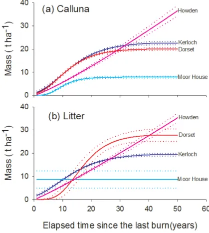
Above-ground biomass accumulation patterns through time since last burn differed be-tween sites (Fig. 2a). These differences, however, were not ordered along the north– south gradient as expected. Moor House, one of the sites with colder temperatures

10

and higher precipitation, had the lowestCallunabiomass values, and grew slowly un-til it reached 20 years after fire with an asymptote around 8 t ha−1. Surprisingly, the two sites at the extremes of the climatic gradient (Kerloch and Dorset) showed inter-mediate and similar accumulations; growth occurred over the first 20 years until an asymptote around 20 t ha−1was achieved approximately 25 years after fire. These two

15

sites were also those that regenerated more quickly and reached the greatest biomass values quicker after fire.Calluna biomass at Howden, the site ranked as the second warmest and driest (after Dorset) had the greatest biomass, increasing linearly until ca. 35 t ha−1was measured 50 years after fire.

Accumulation patterns for litter also differed between sites (Fig. 2b). Although

Cal-20

lunaaccumulation data for Kerloch and Dorset were similar, litter showed different re-sponses. Litter accumulated faster at Kerloch in the first few years towards an asymp-tote at approximately 20 years, whereas in Dorset, litter accumulation followed a clear sigmoidal curve with an early lag phase (0–10 years), and a phase of rapid increase (10–30 years) before reaching an asymptote around 30 years. The asymptotes for

25

(14)

Ker-BGD

12, 17817–17849, 2015

Title Page

Tables Figures

◭ ◮

Back Close

Full Screen / Esc

Discussion

P

a

per

|

Discussion

P

a

per

|

Discussion

P

a

per

|

Discussion

P

a

per

|

loch. At Howden litter increased linearly until ca. 35 t ha−1_{was accumulated 50 years}

after fire, whereas at Moor House litter did not follow any accumulation pattern and was constant through time (ca. 9 t ha−1). The high levels of litter accumulation at Moor House in the first 10 years after fire were considerable and suggest incomplete com-bustion at this site.

5

The predicted, long-term, above-ground fuel load (and associated C_mass) increased for both Calluna and litter with rotation interval for all sites (Fig. 3). As expected, the greatest fuel loads were found in the sites with the largest biomass accumulation rates; i.e. Howden, followed by Dorset and Kerloch, and Moor House with the lowest values. Litter at Moor House was the only fraction not increasing with rotation interval, because

10

its accumulation did not follow any clear temporal pattern (Fig. 3b).

3.2 Hypothesis 2: The optimal prescribed-burning rotation interval will be controlled by the different site-induced patterns of fuel accumulation

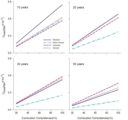
The annual carbon lost through prescribed burning (C_lossPBA) was highly variable de-pending on the site studied (ranging from 0.1 to 0.55 t ha−1, Fig. 4). Two clear patterns

15

were also detected depending on the climatic conditions of sites. At the sites with the lowest temperatures and highest precipitation (Kerloch and Moor House), short rota-tion intervals of ca. 8–10 years maximized carbon emissions. In contrast, the warmer and drier sites (Dorset and Howden) demonstrated a hump-shaped response with the highest C emissions at intermediate rotation intervals. Emissions were maximized in

20

Dorset at ca. 15 year intervals, whereas Howden showed a less pronounced hump-shaped curve with a maximum loss at 15–25 year intervals. Carbon lost was there-fore minimized at long rotation intervals (30–50 years) for all sites, but for Howden and Dorset short prescribed-burning rotation intervals (8–10) can also minimize C losses. As expected, higher combustion completeness (CC) increased the carbon annual loss

25

(15)

BGD

12, 17817–17849, 2015

Title Page

Tables Figures

◭ ◮

Back Close

Full Screen / Esc

Discussion

P

a

per

|

Discussion

P

a

per

|

Discussion

P

a

per

|

Discussion

P

a

per

|

3.3 Hypothesis 3: Wildfire interaction with prescribed-burning rotation interval and its e_ffect on C emissions

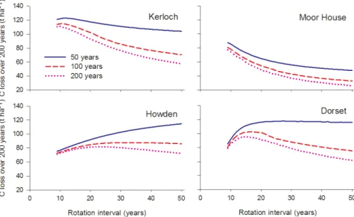
The impact of superimposed wildfires over the prescribed-burning rotations showed that increasing the wildfire frequency increased the carbon loss (C_lossPB200), at all sites; the greatest predicted losses were with a 50 year wildfire return interval, intermediate

5

losses with a 100 year interval and smallest losses with a 200 year interval (Fig. 6). Moreover, at the two sites with warmer and drier conditions (Howden and Dorset), wildfire frequency also modified the range of prescribed-burning rotation intervals at which C loss was minimized. At Howden, C loss at a 200 year wildfire return interval was minimized with prescribed burnings at short- and long-rotation intervals (8 and

10

50 years), and greatest losses were at intermediate rotations (15–25 years). However, shorter wildfire return intervals (50 and 100 years) changed this pattern incrementally. At the 50 year wildfire return interval, C loss increased considerably with lengthening prescribed-burning rotation intervals, the 100 year wildfire return interval produced an intermediate response (Fig. 6); at both return intervals the lowest emissions were

pre-15

dicted at an 8 year prescribed burning rotation frequency (Fig. 6). In Dorset, C loss at a 200 year wildfire return interval was also minimized with prescribed burnings at short- and long-rotation intervals (8 and 50 years), with maximized losses at interme-diate rotations (13–16 years). The predicted pattern was, however, modified at both 100 and 50 year wildfire return intervals. At the 100 year wildfire return interval,

pre-20

scribed burning at short- and long-rotation intervals (8 and 50 years) were minimized C losses, and losses were greatest at prescribed burning rotation intervals between 12 and 22 years. The 50 year wildfire return interval increased C loss at long prescribed-burning intervals, reaching an asymptote of maximized losses at prescribed-prescribed-burning intervals between 15 and 20 years (Fig. 6).

(16)

BGD

12, 17817–17849, 2015

Title Page

Tables Figures

◭ ◮

Back Close

Full Screen / Esc

Discussion

P

a

per

|

Discussion

P

a

per

|

Discussion

P

a

per

|

Discussion

P

a

per

|

4 Discussion

4.1 Hypothesis 1: The latitudinal gradient affects biomass accumulation patterns

Above-groundCallunabiomass accumulation patterns did di_ffer between sites but they did not increase along the north to south gradient as expected; therefore our first

hy-5

pothesis was only partially accepted. Here, three di_fferent responses can be outlined. First, Moor House, with its low mean temperature (8.1◦

C), highest rainfall (1314 mm) and highest altitude ca. 650 m experienced the lowest above-ground biomass accu-mulation. It appears that the Moor House climate and altitude interact to limitCalluna

biomass accumulation (Alday et al., 2015). Second, Kerloch and Dorset, being the

10

most northern and southern sites respectively, with the lowest and warmest mean tem-peratures respectively (7.3 and 10.4◦C), with contrasting rainfall patterns (1040 and 800 mm), experienced similar and intermediateCalluna accumulation rates. The low above-ground biomass production in Dorset has been already attributed to the low fer-tility of its soils (Chapman and Clarke, 1980). We hypothesise that larger biomass

ac-15

cumulation would be expected in Dorset if soils were more fertile. In contrast, it seems that the relative climatic harshness of Kerloch is mainly responsible for the reduced

Callunabiomass accumulation there (Miller, 1979). Finally, the central site of Howden, with intermediate temperatures and rainfall (9◦C and 829 mm), experienced the largest accumulation after 50 years without fire. It is well known that warmer sites experience

20

conditions for growing more vigorous above ground biomass and reach higher amounts of biomass accumulation at longer times since fire. Moreover, Howden, unlike all other sites is surrounded by large industrial conurbations and the area is well known to be affected by past and current industrial pollution including nitrogen deposition (Caporn and Emmett, 2008). Here, therefore, growth responses could be expected to be

arti-25

(17)

BGD

12, 17817–17849, 2015

Title Page

Tables Figures

◭ ◮

Back Close

Full Screen / Esc

Discussion

P

a

per

|

Discussion

P

a

per

|

Discussion

P

a

per

|

Discussion

P

a

per

|

temperature, and reduced by the number of frost days in the previous winter (Palmer, 1997; Milne et al., 2002). Our results indicate that though climate is important in de-terminingCalluna biomass accumulation, it is not necessarily an over-riding, univer-sal explanatory factor at all sites, and other site-specific factors such as soil fertility, pollutant load and altitude (e.g., Moor House; Alday et al., 2015) can significantly

al-5

ter above-ground biomass accumulation patterns. Such site-specific constraints must be considered in future when developing site-specific and national-scale management strategies.

Interestingly, litter accumulation patterns appeared to follow the North-to-South gra-dient; therefore, for litter the first hypothesis is accepted. Kerloch experienced the

high-10

est accumulations in the first years after fire, but with the passage of time, accumulated litter reached an asymptote much lower than southern sites (Howden and Dorset). Moor House, the second most northerly site, did not follow any pattern but its con-stant accumulation through time (around 9 t ha−1) meant high levels of litter in the first 10 years after fire. However, when the data from the northern sites are compared with

15

the two more southerly, warmer sites (Dorset and Howden) accumulation was much lower at longer periods after fire. It is well known that colder and wetter sites can ac-cumulate higher levels of litter in the first stages after fire because the low intensity of fires (cool burns) reduce combustion completeness (Harris et al., 2011), and low decomposition rates. In addition, cold winters can freeze and increase the dieback

20

of manyCalluna leaves, even before reaching senescent states, and increasing sub-sequently litter accumulation (Davies and Legg, 2008). The linkage between above ground biomass and litter accumulated in this study, with very good relationship be-tween them (P <0.001, r2₌0.809), may explain the higher accumulation of litter at longer times in warmer sites; i.e., places with higher above-ground biomass

accumula-25

tion produce more litter through time.

(18)

BGD

12, 17817–17849, 2015

Title Page

Tables Figures

◭ ◮

Back Close

Full Screen / Esc

Discussion

P

a

per

|

Discussion

P

a

per

|

Discussion

P

a

per

|

Discussion

P

a

per

|

prescribed burning rotation interval that maximizes biomass accumulation is the age at which above-ground biomass reaches its asymptote. It was observed that the later the time taken to reach the asymptote, the longer the prescribed-burning rotation interval. Here, theCalluna biomass asymptote for all sites (except Howden) was reached be-tween 20–30 years since the last burn, suggesting that fire-return intervals should be

5

at least as great as theCalluna accumulation asymptote (more than 20 years) (Alday et al., 2015). However, in the case of Howden, its biomass increased progressively with time since the last burn, and consequently the biomass accumulation as func-tion of fire rotafunc-tion interval also followed the same pattern. In any case, these results highlight the importance of studying the biomass accumulation patterns at the

individ-10

ual moorland scale, taking account of site-specific environmental conditions. This will help identify appropriate site-specific fire-rotation intervals, which is fundamental for designing holistic site-specific management plans designed to minimize C loss.

4.2 Hypothesis 2: Annual carbon loss produced by prescribed burning in a particular rotation interval is linked to the pattern of fuel accumulation

15

Annual carbon loss as function of the prescribed fire rotation interval was also vari-able depending on biomass accumulation patterns. The colder sites (Kerloch and Moor House), with greater biomass accumulation in the first years (especially litter), experi-enced greatest annual losses at short rotation intervals (ca. 8–10 years). In contrast, warmer sites (Dorset and Howden) demonstrated a hump-back relationship with largest

20

C losses at intermediate rotation intervals (ca. 15–25 years), and lowest losses at but short- and long- rotation intervals (Fig. 4).

C emission behaviour changed with respect to prescribed burning rotation interval across a considerable part of the latitudinal gradient indicating the difficulties of manag-ing sites usmanag-ing simple prescriptions. The same prescribed burnmanag-ing rotation interval may

25

(19)

BGD

12, 17817–17849, 2015

Title Page

Tables Figures

◭ ◮

Back Close

Full Screen / Esc

Discussion

P

a

per

|

Discussion

P

a

per

|

Discussion

P

a

per

|

Discussion

P

a

per

|

the need for a detailed understanding of biomass accumulation dynamics at the site level to refine burning plans in terms of reducing C emissions. In addition, it is worth noting that the amount of maximum C emitted annually was variable between sites, ranging from 0.38 to 0.53 t ha−1. In this case, higher emission amounts corresponded to sites with fast regeneration immediately after fire (Kerloch and Dorset). Surprisingly,

5

the maximum fuel load reached after a long period without fire seemed unimportant. Finally, as expected, modelling the impact of changing CC during prescribed burn-ing increased significantly the annual C emitted; reachburn-ing a maximum value of 0.85 t ha−1(CC of 100 % at Kerloch with a 10 year rotation interval).This is an increase of between 60 and 123 % over our standard model conditions. The greatest increase

10

in C emissions through simulating a higher CC was found in those sites with fastest regeneration after fire (Kerloch and Dorset) and in short prescribed burning rotation intervals (10 years). The implications of these results are worrying because any small increase in CC can increase C emissions, and increased CC is likely under conditions of global climate change if prescribed burning has to be done in drier, warmer weather.

15

The low CC at Moor House attests to the climatic control of CC in extreme conditions.

4.3 Hypothesis 3: Different wildfire return interval modifies the optimum prescribed burning rotation for reducing annual C loss

Until now we have discussed the relevance of prescribed burning in biomass accu-mulation and C emitted to the atmosphere. However, it is worth noting that prescribed

20

burning is not the only type of fire in British ecosystems, and wildfires produced by accident and arson can occur in spring and summer (Davies and Legg, 2008). These wildfires can be very severe and burn significant amounts of biomass (Maltby et al., 1990). It is important, therefore, to consider the e_ffects of wildfire superimposed on impacts of prescribed burning when modelling C emissions in future scenarios. Here,

25

(20)

BGD

12, 17817–17849, 2015

Title Page

Tables Figures

◭ ◮

Back Close

Full Screen / Esc

Discussion

P

a

per

|

Discussion

P

a

per

|

Discussion

P

a

per

|

Discussion

P

a

per

|

characteristics and the wildfire return interval. For example, in colder sites shorter wild-fire return intervals (50 and 100 year) only increased carbon losses. In warmer sites (Howden and Dorset), shorter wildfire return intervals increased C emissions, but also affected the prescribed-burning rotation interval where C losses were minimized (Ta-ble 2). In Howden and Dorset, for example, whereas at 200 year wildfire interval, long

5

prescribed-burning rotation intervals (ca. 50 years) minimized C emissions, 50 years wildfire return intervals maximized C losses at this rotation interval.

These results, therefore, highlight the uncertainty in establishing fixed prescribed burning rotation intervals at the present time, never mind projecting forward to account for future climate change scenarios or changing wildfire frequency. At present, little is

10

known about the present occurrence of wildfires in Great Britain, but future predictions suggest that these return intervals will be shortened by drier and warmer summers predicted for the future (Jenkins et al., 2009; Krawchuk et al., 2009; Albertson et al., 2011). Further studies are sorely needed to assess future wildfire regime, because it is a key factor required to design suitable management plans to reduce C emissions in

15

fire-prone ecosystems such as heathlands and moorlands.

5 Management implications

Our results provide information to guide policies for the future sustainable manage-ment of European heaths and moors in terms of C budgets. This study suggests that these policies must take into account site-specific characteristics of biomass

produc-20

tion. For sites with cold and wet conditions, long prescribed-burning rotation intervals (ca. every 30–50 years) were optimal for reducing C losses. In contrast, warmer and drier sites, both short- (ca. every 8–10 years) and long- (ca. every 30–50 years) rotation intervals were optimal for reducing C losses; intermediate prescribed burning rotation intervals should be avoided. These results suggest that a further effort for reducing

25

(21)

BGD

12, 17817–17849, 2015

Title Page

Tables Figures

◭ ◮

Back Close

Full Screen / Esc

Discussion

P

a

per

|

Discussion

P

a

per

|

Discussion

P

a

per

|

Discussion

P

a

per

|

intermediate values and close to 20 years (Yallop et al., 2006). In contrast, the present management in Scotland may be optimal in terms C budgets, since the average ro-tation interval is longer, 50–100 years (Hester and Sydes, 1992). In this management planning, it is important to take into account future predictions since climate change suggest that wildfire frequency will increase and this may exacerbate losses. If this

oc-5

curs prescribed burning may only minimize carbon loss if it is applied at short intervals (ca. every 8–10 years) at the warmer and drier sites studied here.

Data availability

Data used for this paper can be freely downloaded from the University of Liverpool research data catalogue, doi:10.17638/datacat.liverpool.ac.uk/58.

10

Acknowledgements. This work would not have been possible without the foresight and per-sistence of staff of the Nature Conservancy, its successor bodies, and the Institute of Ter-restrial Ecology (now the Centre for Ecology & Hydrology). We also thank the Biodiversa (NERC/DEFRA; grant number NE/G002096/1), the Ecological Continuity Trust, the Heather Trust and both the Basque–Country Government (Programa Postdoctoral de perfeccionamiento

15

de doctores del DEUI, BFI- 2010-245) and the Generalitat Valenciana (VAli+d) for post-doctoral awards for JGA and VMS respectively.

References

Albertson, K., Aylen, J., Cavan, G., and McMorrow, J.: Climate change and the future occur-rence of moorland wildfires in the Peak District of the UK, Clim. Res., 45, 105–118, 2011.

20

Alday, J. G., Santana, V. M., Lee, H., Allen, K. A., and Marrs, R. H.: Above-ground biomass accumulation patterns in moorlands after prescribed burning and low-intensity grazing, Per-spect. Plant Ecol. Evol. Syst., 17, 388–396, doi:10.1016/j.ppees.2015.06.007, 2015.

Allen, K. A., Harris, M. P. K., and Marrs, R. H.: Matrix modelling of prescribed burning in Cal-luna vulgaris-dominated moorland: short burning rotations minimize carbon loss at increased

25

(22)

BGD

12, 17817–17849, 2015

Title Page

Tables Figures

◭ ◮

Back Close

Full Screen / Esc

Discussion

P

a

per

|

Discussion

P

a

per

|

Discussion

P

a

per

|

Discussion

P

a

per

|

Anon: Environmental management – guidance: Heather and grass burning: rules and applying for a licence, available at: https://www.gov.uk/heather-and-grass-burning-apply-for-a-licence (last access: 22 May 2015), 2014.

Bain, C. G., Bonn, A., Stoneman, R., Chapman, S., Coupar, A., Evans, M., Gearey, B., Howat, M., Joosten, H., Keenleyside, C., Labadz, J., Lindsay, R., Littlewood, N., Lunt, P.,

5

Miller, C. J., Moxey, A., Orr, H., Reed, M., Smith, P., Swales, V., Thompson, D. B. A., Thomp-son, P. S., Van de Noort, R., WilThomp-son, J. D., and Worrall, F.: IUCN UK Commission of Inquiry on Peatlands, IUCN UK Peatland Programme, Edinburgh, 2011.

Bargmann, T., Måren, I. E., and Vandvik, V.: Life after fire: smoke and ash as germination cues in ericads, herbs and graminoids of northern heathlands, Appl. Veg. Sci., 17, 670–679, 2014.

10

Bond, W. J. and Keeley, J. E.: Fire as a global “herbivore”: the ecology and evolution of flammable ecosystems, Trends Ecol. Evol., 20, 387–394, 2005.

Bowman, D. M., Balch, J. K., Artaxo, P., Bond, W. J., Carlson, J. M., Cochrane, M. A., D’Antonio, C. M., DeFries, R. S., Doyle, J. C., Harrison, S. P., Johnston, F. H., Keeley, J. E., Krawchuk, M. A., Kull, C. A., Marston, J. B., Moritz, M. A., Prentice, I. C., Roos, C. I.,

15

Scott, A. C., Swetnam, T. W., van der Werf, G. R., and Pyne, S. J.: Fire in the earth sys-tem, Science, 324, 481–484, 2009.

Bradstock, R. A., Boer, M. M., Cary, G. J., Price, O. F., Williams, R. J., Barrett, D., Cook, G., Gill, A. M., Hutley, L. B. W., Keith, H., Maier, S. W., Meyer, M., Roxburgh, S. H., and Russell-Smith, J.: Modelling the potential for prescribed burning to mitigate carbon emissions from

20

wildfires in fire-prone forests of Australia, Int. J. Wildland Fire, 21, 629–639, 2012.

Caporn, S. J. M., and Emmett, B. A.: Threats from air pollution and climate change on upland systems – past, present & future, in: Drivers of Environmental Change in Uplands, edited by: Bonn., A., Allott, T., Hubacek, K., and Stewart, J., Routledge, Abingdon, 34–58, 2009. Chapman, S. B.: Nutrient budgets for a dry heath ecosystem in the south of England, J. Ecol.,

25

55, 677–89, 1967.

Chapman, S. B. and Clarke, R. T.: Some relationships between soil, climate, standing crop and organic matter accumulation within a range of Callunaheathlands in Britain, B. Ecol., 11, 221–232, 1980.

Chapman, S. B., Hibble, J., and Rafarel, C. R.: Litter accumulation underCalluna vulgaris on

30

a lowland heathland in Britain, J. Ecol., 63, 259–271, 1975.

(23)

BGD

12, 17817–17849, 2015

Title Page

Tables Figures

◭ ◮

Back Close

Full Screen / Esc

Discussion

P

a

per

|

Discussion

P

a

per

|

Discussion

P

a

per

|

Discussion

P

a

per

|

Davies, G. M. and Legg, C. J.: Developing a live fuel moisture model for moorland fire danger rating, in: Forest fires: modeling, monitoring and management of forest fires, edited by: de las Heras, J., Brebbia, C. A., and Viegas, D. X., WIT Transactions on the Environment, WIT Press, Southampton, 119, 225–236, 2008.

Eriksson, O., Cousins, S. A. O., and Bruun, H. H.: Land-use history and fragmentation of

5

traditionally-managed grasslands in Scandinavia, J. Veg. Sci., 13, 743–748, 2002.

Fernandes, P. M., Davies, G. M., Ascoli, D., Fernandez, C., Moreira, F., Rigolot, E., Stoof, C. R., Vega, J. A., and Molina, D.: Prescribed burning in southern Europe: developing fire manage-ment in a dynamic landscape, Front. Ecol. Environ., 11, e4-e14, 2013.

Galford, G. L., Melillo, J. M., Kicklighter, D. W., Cronin, T. W., Cerri, C. E., Mustard, J. F., and

10

Cerri, C. C.: Greenhouse gas emissions from alternative futures of deforestation and agri-cultural management in the southern Amazon, P. Natl. Acad. Sci. USA, 107, 19649–19654, 2010.

Gimingham, C. H.: Ecology of Heathlands, Chapman and Hall, London, 1972.

Harris, M. P. K., Allen, K. A., McAllister, H. A., Eyre, G., Le Duc, M. G., and Marrs, R. H.:

Fac-15

tors affecting moorland plant communities and component species in relation to prescribed burning, J. Appl. Ecol., 48, 1411–1421, 2011.

Heal, O. W. and Perkins, D. F.: Production Ecology of British Moors and Montane Grasslands, Springer, Berlin, 1978.

Heal, O. W. and Smith, R. A. H.: Introduction and site description, in: Production Ecology of

20

British Moors and Montane Grasslands, edited by: Heal, O. W., and Perkins, D. F., Springer, Berlin, 36–18, 1978.

Hester, A. J. and Sydes, C.: Changes in burning of Scottish heather moorland since the 1940s from aerial photographs, Biol. Conserv., 60, 25–30, 1992.

Holdridge, L. R.: Determination of world plant formation from simple climate data, Science, 105,

25

367–368, 1947.

Hill, M. O.: TABLEFIT: For Identification of Vegetation Types (v.1.1), Centre for Ecology and Hydrology, Wallingford, 2011.

Jenkins, G. J., Murphy, J. M., Sexton, D. M. H., Lowe, J. A., Jones, P., and Kilsby, C. G.: UK Climate Projections: Briefing Report, Met Office Hadley Centre, Exeter, 2009.

30

(24)

BGD

12, 17817–17849, 2015

Title Page

Tables Figures

◭ ◮

Back Close

Full Screen / Esc

Discussion

P

a

per

|

Discussion

P

a

per

|

Discussion

P

a

per

|

Discussion

P

a

per

|

Krawchuk, M. A., Moritz, M. A., Parisien, M.-A., Van Dorn, J., and Hayhoe. K.: Global pyrogeog-raphy: the current and future distribution of wildfire, PLoS One, 4, e5102, 2009.

Lee, H., Alday, J. G., Rose, R. J., O’Reilly, J., and Marrs, R. H.: Long-term effects of rotational prescribed-burning and low-intensity sheep-grazing on blanket-bog plant communities, J. Appl. Ecol., 50, 625–635, 2013.

5

Leslie, P. H.: On the use of matrices in certain population mathematics, Biometrika, 35, 183– 212, 1945.

Maltby, E., Legg, C. J., and Proctor, M. C. F.: The ecology of severe moorland fire on the North York Moors: effects of the 1976 fires, and subsequent surface and vegetation development, J. Ecol., 78, 490–518, 1990.

10

Miller, G. R.: Quantity and quality of the annual production of shoots and flowers byCalluna vulgarisin north-east Scotland, J. Ecol., 67, 109–129, 1979.

Milne, J. A., Pakeman, R. J., Kirkham, F. W., Jones, I. P., and Hossell, J. E.: Biomass production of upland vegetation types in England and Wales, Grass Forage Sci., 57, 373–388, 2002. Natural England: The Heather and Grass Burning code, available at: http://publications.

15

naturalengland.org.uk/publication/4719598414856192 (last access: 23 May 2015), 2007. Palmer, S. C. F.: Prediction of the shoot production of heather under grazing in the uplands of

Great Britain, Grass Forage Sci., 52, 408–424, 1997.

Pan, Y., Birdsey, R. A., Fang, J., Houghton, R., Kauppi, P. E., Kurz, W. A., Phillips, O. L., Shvidenko, A., Lewis, S. L., Canadell, J. G., Ciais, P., Jackson, R. B., Pacala, S. W.,

20

McGuire, A. D., Piao, S., Rautiainen, A., Sitch, S., and Hayes, D.: A large and persistent carbon sink in the world’s forests, Science, 333, 988–993, 2011.

Pausas, J. G. and Ribeiro, E.: The global fire–productivity relationship, Global Ecol. Bio-geogr., 22, 728–736, 2013.

Pinheiro, J. C. and Bates, D. M.: Mixed Effects Models in S and S-PLUS, Springer, New York,

25

2000.

Post, W. M., Izaurralde, R. C., West, T. O., Liebig, M. A., and King, A. W.: Management op-portunities for enhancing terrestrial carbon dioxide sinks, Front. Ecol. Environ., 10, 554–561, 2012.

R Core Team.: R: A language and environment for statistical computing, R Foundation for

Sta-30

(25)

BGD

12, 17817–17849, 2015

Title Page

Tables Figures

◭ ◮

Back Close

Full Screen / Esc

Discussion

P

a

per

|

Discussion

P

a

per

|

Discussion

P

a

per

|

Discussion

P

a

per

|

Rodwell, J. S.: British Plant Communities Vol. 2: Mires and Heaths, Cambridge University Press, Cambridge, 1991.

Rosenburgh, A., Alday, J. G., Harris, M. P. K., Allen, K. A., Connor, L., Blackbird, S., Eyre, G., and Marrs, R. H.: Changes in peat chemical properties during post-fire succession on blanket bog moorland, Geoderma, 211–212, 98–106, 2013.

5

Schimel, D. S., House, J. I., Hibbard, K. A., Bousquet, P., Ciais, P., Peylin, P., Braswell, B. H., Apps, M. J., Baker, D., Bondeau, A., Canadell, J., Churkina, G., Cramer, W., Denning, A. S., Field, C. B., Friedlingstein, P., Goodale, C., Heimann, M., Houghton, R. A., Melillo, J. M., Moore III, B., Murdiyarso, D., Noble, I., Pacala, S. W., Prentice, I. C., Raupach, M. R., Rayner, P. J., Scholes, R. J., Steffen, W. L., and Wirth, C.: Recent patterns and mechanisms

10

of carbon exchange by terrestrial ecosystems, Nature, 414, 169–172, 2001.

Schimel, D. and Baker, D.: Carbon cycle: the wildfire factor, Nature, 420, 29–30, 2002.

Scottish Government: The Muirburn Code, available at: http://www.gov.scot/Publications/2011/ 08/09125203/0 (last access: 23 May 2015), 2011.

Stewart, G. B., Coles, C. F., and Pullin, A. S.: Applying evidence-based practice in

conserva-15

tion management: lessons from the first systematic review and dissemination projects, Biol. Conserv., 126, 270–278, 2005.

Tucker, G. T.: Review of the impacts of heather and grassland burning in the uplands on soils, hydrology and biodiversity, English Nature Research Report No. 55, Natural England, Peter-borough, 2003.

20

van der Werf, G. R., Randerson, J. T., Giglio, L., Collatz, G. J., Mu, M., Kasibhatla, P. S., Morton, D. C., DeFries, R. S., Jin, Y., and van Leeuwen, T. T.: Global fire emissions and the contribu-tion of deforestacontribu-tion, savanna, forest, agricultural, and peat fires (1997–2009), Atmos. Chem. Phys., 10, 11707–11735, doi:10.5194/acp-10-11707-2010, 2010.

Vandvik, V., Heegaard, E., Måren, I. E., and Aarrestad, P. A.: Managing heterogeneity: The

25

importance of grazing and environmental variation on post-fire succession in heathlands, J. Appl. Ecol., 42, 139–149, 2005.

Watt, A. S.: Pattern and process in the plant community, J. Ecol., 35, 1–22, 1947.

Watt, A. S.: Bracken versus heather: a study in plant sociology, J. Ecol., 43, 490–506, 1955. Yallop, A. R., Thacker, J. I., Thomas, G., Stephens, M., Clutterbuck, B., Brewer, T., and

San-30

(26)

BGD

12, 17817–17849, 2015

Title Page

Tables Figures

◭ ◮

Back Close

Full Screen / Esc

Discussion

P

a

per

|

Discussion

P

a

per

|

Discussion

P

a

per

|

Discussion

P

a

per

|

Table 1.Parameters of the selected models for biomass accumulation patterns through time since the last burning (years). Data from the selected four sites in Great Britain was modelled independently.(a)Callunabiomass (t ha−1

) and(b)litter biomass (t ha−1

)

(a)Callunabiomass (b)Litter

Site Model selected a b c Model selected a b c

Kerloch Gompertz Estimate 22.96 3.22 0.88 Gompertz Estimate 20.65 2.61 0.89

SE 0.89 0.46 0.01 SE 0.79 0.31 0.01

tvalue 25.62 6.97 67.09 tvalue 26.12 8.21 72.49 P <0.001 <0.001 <0.001 P <0.001 <0.001 <0.001

Moor House Gompertz Estimate 7.94 8.07 0.78 No model selected SE 0.80 3.55 0.04

tvalue 10.08 2.28 20.12 P <0.001 0.035 <0.001

Howden Linear Estimate −0.93 1.15 – Linear Estimate 3.86 1.1 – [log(y)∼log(x+1)] SE 0.05 0.02 – [log(y)∼log(x+1)] SE 0.04 0.02 – tvalue −19.98 48.14 – tvalue 92.61 51.32 – P <0.001 <0.001 – P <0.001 <0.001 –

Dorset Gompertz Estimate 20.15 3.58 0.86 Gompertz Estimate 28.38 8.67 0.86

SE 0.62 0.53 0.01 SE 2.96 6.11 0.04

(27)

BGD

12, 17817–17849, 2015

Title Page

Tables Figures

◭ ◮

Back Close

Full Screen / Esc

Discussion

P

a

per

|

Discussion

P

a

per

|

Discussion

P

a

per

|

Discussion

P

a

per

|

Table 2.Optimal prescribed burning rotation interval where C losses over 200 years (ClossPB200)

are minimized. These optimal rotation intervals are calculated including the incidence of wild-fires at three different return intervals 50, 100 and 200 years.

Wildfire return interval

Site Optimal prescribed burning rotation interval (years)

ClossPB200(t ha

−1

)

50 years Kerloch 50 103

Moor House 50 48

Howden 8 75

Dorset 8 85

Moor House 50 33

Howden 8 72

Dorset 8 and 50 81 and 75

Moor House 50 26

Howden 8 and 50 71 and 72

(28)

BGD

12, 17817–17849, 2015

Title Page

Tables Figures

◭ ◮

Back Close

Full Screen / Esc

Discussion

P

a

per

|

Discussion

P

a

per

|

Discussion

P

a

per

|

Discussion

P

a

per

|

(29)

BGD

12, 17817–17849, 2015

Title Page

Tables Figures

◭ ◮

Back Close

Full Screen / Esc

Discussion

P

a

per

|

Discussion

P

a

per

|

Discussion

P

a

per

|

Discussion

P

a

per

|

(30)

BGD

12, 17817–17849, 2015

Title Page

Tables Figures

◭ ◮

Back Close

Full Screen / Esc

Discussion

P

a

per

|

Discussion

P

a

per

|

Discussion

P

a

per

|

Discussion

P

a

per

|

Figure 3.Predicted long-term modelled above-ground fuel load and carbon mass of(a)Calluna

(31)

BGD

12, 17817–17849, 2015

Title Page

Tables Figures

◭ ◮

Back Close

Full Screen / Esc

Discussion

P

a

per

|

Discussion

P

a

per

|

Discussion

P

a

per

|

Discussion

P

a

per

|