The Cryosphere, 7, 977–986, 2013 www.the-cryosphere.net/7/977/2013/ doi:10.5194/tc-7-977-2013
© Author(s) 2013. CC Attribution 3.0 License.
Geoscientiic
Geoscientiic
Geoscientiic
The Cryosphere
Open Access
Variability of light transmission through Arctic land-fast sea ice
during spring
M. Nicolaus1, C. Petrich2, S. R. Hudson3, and M. A. Granskog3
1Alfred-Wegener-Institut, Helmholtz-Zentrum f¨ur Polar- und Meeresforschung, Bremerhaven, Germany 2Norut Narvik AS, Narvik, Norway
3Norwegian Polar Institute, Fram Centre, Tromsø, Norway
Correspondence to:M. Nicolaus ([email protected])
Received: 17 September 2012 – Published in The Cryosphere Discuss.: 12 October 2012 Revised: 16 May 2013 – Accepted: 17 May 2013 – Published: 20 June 2013
Abstract.The amount of solar radiation transmitted through Arctic sea ice is determined by the thickness and physi-cal properties of snow and sea ice. Light transmittance is highly variable in space and time since thickness and physi-cal properties of snow and sea ice are highly heterogeneous on variable time and length scales. We present field mea-surements of under-ice irradiance along transects under un-deformed land-fast sea ice at Barrow, Alaska (March, May, and June 2010). The measurements were performed with a spectral radiometer mounted on a floating under-ice sled. The objective was to quantify the spatial variability of light trans-mittance through snow and sea ice, and to compare this vari-ability along its seasonal evolution. Along with optical mea-surements, snow depth, sea ice thickness, and freeboard were recorded, and ice cores were analyzed for chlorophylla and particulate matter. Our results show that snow cover variabil-ity prior to onset of snow melt causes as much relative spatial variability of light transmittance as the contrast of ponded and white ice during summer. Both before and after melt on-set, measured transmittances fell in a range from one third to three times the mean value. In addition, we found a twen-tyfold increase of light transmittance as a result of partial snowmelt, showing the seasonal evolution of transmittance through sea ice far exceeds the spatial variability. However, prior melt onset, light transmittance was time invariant and differences in under-ice irradiance were directly related to the spatial variability of the snow cover.
1 Introduction
still the subject of various studies, in particular with respect to its spatial and spectral variability. This is because most studies of the last decades have concentrated on land-fast or multi-year pack ice.
Compared to surface albedo, little is known about the spa-tial and temporal variability of the amount of solar irradiance under sea ice (Ehn et al., 2011; Gradinger et al., 2009; Hud-son et al., 2013; Light et al., 2008; Nicolaus et al., 2010a; Per-ovich et al., 1998). One major challenge is accessibility of the under-ice environment, such that measurements are mostly limited to time-consuming spot measurements through bore holes. As a result, biologically and climatologically relevant energy budgets of specific regions and seasons cannot be given yet. A first comprehensive understanding of under-ice irradiance was achieved using data from SHEBA (Surface Heat Budget of the Arctic Ocean) and radiative transfer sim-ulations (Light et al., 2008). The first successful, long-term observations of transmitted irradiance through Arctic sea ice by an autonomous station, part of the drift ofTarain 2007, show a seasonality inverse to that of surface albedo and high-light the importance of biological processes and their timing (Nicolaus et al., 2010a, b).
The first detailed studies of spatial variability of light transmission through sea ice were performed under land-fast sea ice off Barrow, Alaska, by Perovich et al. (1998) and Maykut and Grenfell (1975). Maykut and Grenfell (1975) performed their measurements in early June 1972. They highlight the role of surface properties for light transmit-tance, and demonstrate the general shapes of spectra of trans-mitted irradiance for seasonally-evolving surface conditions. Perovich et al. (1998) observed highly variable total trans-mittances between 0.0005 and 0.008 during April. This vari-ability was mainly caused by differences in snow depth. Pet-rich et al. (2012b) showed through Monte Carlo simulations that light conditions at the bottom of sea ice are influenced by snow and sea-ice properties within a radius of 1 to 2 m. They also highlight the importance of sea-ice texture in the bottommost decimeters on shaping the light field and light spreading under sea ice. Transmittance measurements through pond-covered sea ice, performed by divers, allowed to quantify light transmittance and the spreading of light un-der sea ice in orun-der to describe the light environment unun-der highly heterogeneous ponded and white ice during summer (Ehn et al., 2011; Hudson et al., 2013). The most comprehen-sive data set of spectral radiation data under melt-pond cov-ered summer Arctic sea ice with a focus on spatial variabil-ity was presented by Nicolaus et al. (2012). Their analyses focused on the large-scale difference of first-year ice (FYI) and multi-year ice (MYI), showing that FYI transmits three times more light than MYI. This results from different opti-cal properties, reduced sea-ice thickness (smaller freeboard), and higher surface coverage of melt ponds on FYI.
At the same time, connections between physical, biolog-ical, and optical properties of sea ice have long been rec-ognized (Grenfell and Maykut, 1977; Maykut and Grenfell,
1975). Also more recent studies (Arrigo et al., 2012; Mundy et al., 2009) have highlighted the role of light for under-ice habitats and the timing of algal blooms under sea ice. The amount of sunlight transmitted though snow and sea ice into the upper ocean is of great importance for primary productiv-ity and biogeochemical fluxes (Arrigo et al., 1991; Gradinger et al., 2009; Uusikivi et al., 2010), because it is the primary energy source for photosynthesis. Based on this, there is an ongoing discussion on how changing ice conditions and the increasing light availability under sea ice (Nicolaus et al., 2012) might alter primary productivity. Under-ice measure-ments of solar irradiance have also been used to calculate biomass at the bottom of sea ice as a non-destructive method (Mundy et al., 2007).
However, comparisons across transmittance studies is of-ten hampered by the variability of snow, sea-ice, and weather conditions, and the need for combined studies of spatial vari-ability and seasonal evolution arises. The goal of the present study is to quantify the spatial and seasonal variability of solar short-wave transmittance through Arctic sea ice. To accomplish this, we performed in-situ measurements of so-lar irradiance along horizontal transects under undeformed land-fast sea ice off Barrow, Alaska, in March, May, and June 2010. These measurements represent ice conditions be-fore and after melt onset, but bebe-fore melt ponds formed. Our analyses quantify spatial and temporal variability of light transmission, focusing on the range of photosynthetically ac-tive radiation (PAR, 400 to 700 nm).
2 Methods
Measurements were performed on level, seasonal, land-fast sea ice at the site of the sea-ice observatory at Barrow, Alaska (Druckenmiller et al., 2009), on 22 March, 14 May, and 11 June 2010. The site was chosen for the availabil-ity of supplementary data from seasonally installed radia-tion and ice mass balance staradia-tions. These staradia-tions provided a local record of incident, reflected, and transmitted spectral irradiance (Nicolaus et al., 2010b), ice thickness, tempera-ture, snow depth, and atmospheric data (Druckenmiller et al., 2009). Water depth was approximately 6 m.
Incident and transmitted solar irradiance were measured simultaneously with two upward-looking Ramses spectral ra-diometers with advanced cosine collectors (Ramses ACC, Trios GmbH, Rastede, Germany). Sensors, data process-ing, and data quality are discussed in detail by Nicolaus et al. (2010b). One sensor was mounted on a buoyant sled and operated under the sea ice (under-ice irradiance, ET, with
“T” for transmitted≡Ed (bottom, 400–700 nm)), and one
sensor was mounted stationary as surface reference (incident solar irradiance, ES, with “S” for surface ≡ Ed (surface,
Fig. 1. (a)Sled lying on its side with radiometer in the center, a backward-looking on-board camera, and the yellow tether line at the back of the sled. The straps tie the propulsion to the sled (motor, speed controller and weights).(b)Photograph taken by the on-board camera during under-ice operations in June. The underside of the ice close to the sensor is white while ice in the distance appears to be cyan presumably because of preferential absorption of red light in water.
et al. (2010b). The distance between the radiometer on the sled and the ice bottom was 2±1 cm, varying slightly with under-ice topography. Spectra were not corrected for absorp-tion between the sensor and the ice bottom, because of the very small distance and the expected uncertainties related to such corrections (Nicolaus and Katlein, 2013). The under-ice radiometer was equipped with an additional inclination and pressure module (type SAMIP, Nicolaus et al., 2010b). From these pressure measurements, the depth of the radiometer and finally sea-ice draft was obtained for each spectrum.
The radiometer sled consisted of a buoyant frame with a centered hole for the radiometer, a means of propulsion that was controlled through a tether line, and an avalanche transmitter (Pieps DSP, Lebring, Austria; UHF transmitter as used in mountaineering to locate people buried by snow avalanches) for under-ice localization. Figure 1 shows the setup used in June. The sled was deployed through a rect-angular access hole cut through the ice (Fig. 2). Prior to the measurements, the sled was propelled forward with electric motors until it became stuck or reached the end of the tether. Then the motors were turned off. Due to the simple construc-tion, the sled was not able to move laterally or vertically. At the transect’s end, the first radiation measurements were trig-gered synchronously for the under- and above-ice sensors. Afterwards, the horizontal position of the sled (and radiome-ter) was determined with an avalanche receiver by search-ing for it from the ice surface with least possible destruction of the snow and ice surface. Actual tether length and direc-tion eased the search procedure. Then the sled was manu-ally pulled toward the access hole at increments of nomi-nally 0.5 m. After each 0.5 m pull, both sensors were again triggered. The along-transect coordinate is the nominal path distance of the radiometer from the access hole. During tran-sect measurements, the horizontal position of the under-ice radiometer was determined with an avalanche receiver (accu-racy approximately 0.2 m) every 5 to 10 m. These tie points
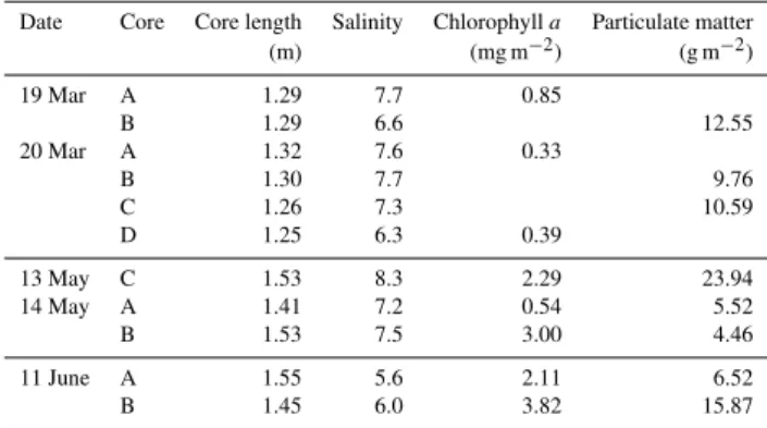
Table 1.Vertically integrated sea-ice properties from all full-length cores obtained during the measurements in 2010. Missing values were not measured. Full profile data are available online (http://dx. doi.org/10.1594/PANGAEA.780223).
Date Core Core length Salinity Chlorophylla Particulate matter (m) (mg m−2) (g m−2)
19 Mar A 1.29 7.7 0.85
B 1.29 6.6 12.55 20 Mar A 1.32 7.6 0.33
B 1.30 7.7 9.76
C 1.26 7.3 10.59 D 1.25 6.3 0.39
13 May C 1.53 8.3 2.29 23.94 14 May A 1.41 7.2 0.54 5.52 B 1.53 7.5 3.00 4.46
11 June A 1.55 5.6 2.11 6.52 B 1.45 6.0 3.82 15.87
were marked at the snow surface. After all measurements were completed, the exact distances from the marks to the ac-cess hole were measured with a tape measure. Measurements were performed around solar noon, and it took approximately 1.5 h to complete the transect.
On 22 March, the access hole was located in the middle of the transect (Figs. 2a, 3a). Starting from this hole, two transects, one 36 m and one 32 m long, were measured un-der clear-sky conditions. The transects headed in different directions from the access hole. Transect length was limited by under-ice topography that could not be passed since the sled had no means of vertical navigation. These two profiles were combined into one transect, consisting of 117 coinci-dent measurements of incicoinci-dent and transmitted spectra. On 14 May, the access hole was at one end of an 80 m long transect (123 measurements, Figs. 2b, 3b) and the measure-ments were performed under overcast conditions with thin clouds. This transect length was limited by the cable length. On 11 June, two 20 m-long transects were measured in sim-ilar directions from the access hole (Figs. 2c, 3c), because a strong current forced the sled in one particular direction. Transect lengths were again limited by under-ice topography. These two sub-profiles were combined into one transect, con-sisting of 71 paired spectral measurements. Cloud conditions were variable with changing fractions of clouds obstructing the solar disk. A compact camera was attached to the sled in June and programmed to take one photograph every 10 s. Flash was disabled and an indicator light on the camera was covered to prevent interference with optical measurements. The ice underside, the radiometer and parts of the sled were in the field of view; the camera was oriented toward the ac-cess hole (Fig. 1b).
Fig. 2. Photographs of surface conditions along profiles in (a) March,(b)May, and(c)June 2010. All photographs were taken af-ter completion of the measurements, which were performed under undisturbed surfaces. The snow pile next to the hole in June resulted from the hole construction. This part was removed for analyses.
of the site of the observatory and within 50 m of each other, on uniform ice. Since data sets have different spatial resolu-tions, snow and ice data were interpolated to derive a total ice thickness and snow depth at the locations of the spectral measurements. Observations that were obviously influenced by the access hole (within 2 to 5 m) were not included.
After each transect, a number of sea-ice cores were re-trieved along the profiles for salinity, chlorophylla(Chla), and particulate measurements (Table 1). In March, six cores were taken within a few meters of the access hole. In May and June three and two cores were taken along the tran-sects, respectively. All optical, thickness, and ice-core data are available online from the Pangaea data publishing sys-tem under http://dx.doi.org/10.1594/PANGAEA.780223.
3 Results and discussion
3.1 Thickness and melt of snow and sea ice
In March, the mean and standard deviation of sea-ice thick-ness was 1.28±0.06 m, snow depth was 0.22±0.08 m, and freeboard was mostly positive (Figs. 3, 4). By May, sea-ice thickness increased to 1.47±0.06 m and snow depth in-creased to 0.27±0.06 m, while modal snow depth remained unchanged at 0.25 m. Regular visits and measurements of surface albedo show that surface melt started after 5 June, with the first melt ponds forming on 09 June (Polashenski et al., 2012), causing a reduction in mean snow depth to 0.07±0.03 m by the June measurements. Sea-ice thickness increased slightly to 1.50±0.02 m. Freeboard was positive along the entire profile. The histograms in Fig. 4 illustrate that the range of sea-ice thickness and snow depth along the transects was largest in March and smallest in June. Changes in snow depth and snow properties can be seen in the pho-tographs of surface conditions in Fig. 2, showing a visibly lower albedo and wet snow in June. These changes are
ex-Table 2.Incident solar radiation fluxes above (ES,PAR) and under (ET,PAR) sea ice, as well as transmittance (TPAR) of photosynthetic
active radiation (PAR).
22 Mar 14 May 11 Jun
n Number of measurements 117 123 71
ES,PAR Mean (W m−2) 153.1 262.4 229.8
Std (W m−2) 8.0 33.4 30.7 Min (W m−2) 141.1 214.3 194.8 Max (W m−2) 161.1 327.8 332.7
ET,PAR Mean (W m−2) 0.34 0.49 9.40
Std (W m−2) 0.36 0.17 4.28 Min (W m−2) 0.06 0.16 3.87 Max (W m−2) 1.80 0.94 17.50
TPAR Mean 0.0022 0.0019 0.041
Std 0.0022 0.0006 0.019 Min 0.0004 0.0006 0.014 Max 0.0113 0.0035 0.086
pected to strongly influence the optical measurements under the sea ice, presented below.
3.2 Sea-ice properties
Sea-ice salinity profiles measured during the March cam-paign showed C-shaped profiles typical of seasonal ice dur-ing the growth season, with the highest salinity of about 12 in the uppermost 0.05 m and a mean salinity of 7.2 (Table 1). In May, salinity profiles were very similar to the ones measured in March, containing just slightly more salt (mean 7.7). This indicates little if any flushing of sea ice until after our May transect. However, by 11 June the mean salinity decreased to 5.8, indicative of flushing. Physical inspection of the ice un-derside in June showed a thinner and less pronounced layer of brittle sea-ice lamellae (not fully consolidated ice crys-tals) than in March and May, with less biota visible than in May but more than in March. Vertically integrated Chla
Fig. 4.Frequency distributions of(a)sea-ice thickness and(b)snow depth(c)transmitted irradiance of PAR, and(d) transmittance of PAR along the transects. Mean values of all distributions are given as mean±one standard deviation in the legends.
3.3 Solar irradiance above and below sea ice
Incident PAR irradiance at the surface,ES,PAR, varied
be-tween the three campaigns. Due to differences in sky con-ditions, ES,PAR was higher in May than in June. Also the
degree of variability in ES,PAR differed during the
mea-surements; ES,PAR varied only slightly (153±8 W m−2,
705 µE s−1m−2,±denotes one standard deviation) in March under clear sky conditions, while ES,PAR was more
vari-able in May (262±33 W m−2, 1207 µE s−1m−2)and June (230±31 W m−2, 1059 µE s−1m−2), when the skies were overcast with changing cloud cover (Table 2). Transmitted solar irradiance recorded under sea ice, ET, varied
signifi-cantly along each transect (spatial variability) and between the three transects (temporal evolution). Figure 3 shows the results of the under-ice measurements and illustrates the ob-served variability along each transect for three selected wave-lengths in the PAR range (400, 550, and 700 nm) and for the total transmitted PARET,PAR. This variability was very
pro-nounced in March, when the first profile (negative x values) had a range of ET,PAR up to 1.8 W m−2 (8.3 µE s−1m−2)
while the second profile had very little variability with all fluxes below 0.5 W m−2(2.3 µE s−1m−2). The largest fluxes were observed in June, when ET,PAR ranged from 3.9 to
17.5 W m−2(18.0 to 81 µE s−1m−2)(Table 2).
Comparing the three measurement dates, ET,PAR
in-creased from 0.34±0.36 W m−2(1.8 µE s−1m−2)in March
Fig. 5. Spectral transmittance through snow and sea ice in (a) March,(b)May, and(c)June 2010. For each transect the spectra for minimum and maximum light conditions as well as the mean spectrum for the transect are given. Note different scales (factor 10) for the data in June.
to 0.49±0.17 W m−2 (2.5 µE s−1m−2) in May, and to 9.40±4.28 W m−2 (50 µE s−1m−2)in June (Fig. 4). Most significant here is the increase by a factor of 20 from March and May to June. This increase in absolute fluxes was mostly related to changing snow conditions and was not primarily a consequence of higher sun elevation in June. Overcast con-ditions resulted in even lowerES,PAR in June than in May,
while under-ice fluxes were highest in June (Table 2). This observation also represents the transition from before to af-ter melt onset conditions. While these fluxes quantify light transmission through sea ice along the profiles, it is difficult to distinguish between an increase ofETdue to the seasonal
increase ofES and the effect of seasonal changes in optical
properties of snow and sea ice along the transects. Hence, we will concentrate on changes in mean transmittance of PAR,
TPAR=ET,PAR/ES,PAR, in this manuscript, in order to
as-sess the spatial variability and seasonal evolution in more de-tail.
3.4 Spectral and PAR transmittance
were similar to those observed in the transpolar drift in 2007 (Nicolaus et al., 2010a) for the same time of the year.
Mean transmittances of PAR,TPAR, were very similar in
March (0.0022) and May (0.0019) (Fig. 4d), although the March value is strongly influenced by a section with thin snow and particularly high transmittance (Figs. 3a, 4b, 4d). Maximum values ofTPARwere 3 times higher in March than
in May due to this region with thinner snow, but minimum and modal values are similar (Fig. 5a, b). The mode ofTPAR
(lowest bin, Fig. 4d) remained the same (within the given resolution of 0.01), combining the effects of a moderate de-crease in modal snow thickness, from 0.28 to 0.24 m, and a slight increase in modal sea-ice thickness, by 0.19 m. Com-paring TPAR before and after melt onset (but before
melt-pond formation along the transect), the values in March and May were over one order of magnitude lower than in June. In contrast to the small modal changes inTPARfrom March to
May, every observedTPARin June (0.014 to 0.086) was larger
than the maximum in March or May (Fig. 4d). Qualitatively, the same results hold for all wavelengths (Fig. 5). This in-crease occurred despite an inin-crease of 0.22 m (17 %) in sea-ice thickness from March to June, as this small increase in sea-ice thickness was more than offset by a 0.15 m (67 %) decrease in snow depth, illustrating the dominating role of snow in de-termining transmittance at this time of the year. Extinction coefficients for PAR are not presented here, as it is not possi-ble to distinguish the different effects of snow and sea ice in this study.
3.5 Spatial vs. seasonal variability
Based on the three transects at three different dates over the course of the season, it was – to our knowledge for the first time – possible to compare the spatial and temporal variabil-ity of light transmittance through sea ice. It may be con-cluded that (1) prior to melt onset (i.e., March and May), the spatial variability (comparing minimum, mean, and max-imum ofTPAR)did not change significantly with time and
(2) the relative spatial variability was constant even through the transition into the melt season. The ratio ofTPAR
min-ima/maxima and meanTPAR was about 5 in March, 2 to 3
in May and 2 in June. Hence relative variability was approx-imately the same before and after melt onset, i.e., ranging from about one third to three times the mean value. In ad-dition, the seasonal increase of transmittance of one order of magnitude in response to melt onset (from March/May to June) was much larger than the relative spatial variability along the transects.
Our observed variability in transmittance through spring snow and sea ice off Barrow, Alaska, matches well the re-sults of Perovich et al. (1998) for the same region and season (April, before melt onset), which showed a variability be-tween 0.0005 and 0.007 in transmittance along a 125 m-long transect. These ranges represent the uncertainty that should be expected for a single spot measurement of under-ice
ra-diation (e.g., Gradinger et al., 2009; Light et al., 2008) or stationary setups (Nicolaus et al., 2010a). Variability contin-ues to evolve further into the melt season, when enhanced melting results in distinct areas of melt ponds and white ice. Observations by Ehn et al. (2011) show PAR transmit-tances of 0.05 to 0.16 for snow free white ice and 0.38 to 0.67 for melt ponds for first-year ice in the Canadian Arc-tic. While Hudson et al. (2013) report for thin Arctic first-year sea ice transmittances (broadband) of 0.11 and 0.39 for bare ice and melt ponds, respectively. These numbers indi-cate similar variability as observed here, indicating that pre-melt snow cover variations may cause as much relative spa-tial variability as the contrast of ponded and bare ice with surface scattering layer (white ice) summer sea ice. Nicolaus et al. (2012) found a larger variability at the end of the melt season, when a bi-modal distribution of transmittances was found, with peaks for ponded and white ice. Modal transmit-tance through ponds was 5 (MYI) to 14 (FYI) times higher than through white ice. In addition, a wide range of transmit-tance variability was observed (but not quantified) within the white ice and ponded ice. However, the data set as a whole is difficult to compare, since it comprises a much boarder range of snow and ice conditions than in this study.
For a detailed comparison of under-ice irradiance with snow depth, the horizontal spreading of light in sea ice has to be considered. This spread results in a 1 to 2 m footprint of the measurement, depending on ice-cover properties and so-lar zenith and azimuth angles (Ehn et al., 2011; Petrich et al., 2012b). Since this is less than the spatial correlation length of snow features (e.g., Petrich et al., 2012a; Sturm et al., 2002), optical measurements can be interpreted based on locally av-eraged snow depths in addition to ice thickness and ice type observations.
Comparing the spatial variability with the 20-fold seasonal increase of transmittances from March to June (prior to melt-pond formation), it may be concluded that inter-seasonal variability is much larger than spatial variability when the melt season is included in considerations. For comparison, during the transpolar drift ofTara in 2007 (Nicolaus et al., 2010a), transmittance of PAR increased from 0.003 before melt onset, to 0.056 after melt onset when the surface was al-most entirely ponded. This also represents a 20-fold increase of PAR transmittance over the course of seasons, but on MYI and without consideration of spatial variability.
snow is a nearly wavelength-independent reduction of vis-ible and near-UV transmittance, wavelengths at which ab-sorption is low in pure ice and extinction is dominated by scattering, which is nearly wavelength independent (Warren et al., 2006). At longer wavelengths, where the absorption coefficient of ice increases, the significance of snow depth is reduced on thick ice since light will be absorbed by sea ice.
3.6 Biomass estimates
In order to estimate sea-ice biomass from the optical mea-surements, the method of normalized difference indices (NDIs) was applied, as suggested by Mundy et al. (2007) based on data from Resolute Passage. Correlating these dices with snow depths, it was possible to show the in-dependence of the method from snow depth and snow properties (data not shown). However, calculated biomass estimates from the spectral measurements exceeded mea-surements by an order of magnitude. Mean concentrations along the transects would be 43.1±7.8 mg m−2for March, 45.7±7.3 mg m−2for May, and 63.7±2.6 mg m−2for June (compared to the measurements summarized in Table 1). It is assumed that the main reasons for this are (1) Chla con-centrations in this study (<3 mg m−2)were too low to allow the application of the algorithm from Resolute Passage (up to 110 mg m−2), (2) the high load of particulate matter (up to
24 g m−2)in this study can affect spectral transmittance, (3)
biological processes that change the pigment composition, e.g., regional differences in algal communities, and (4) non-linear aggregate effects exist at high abundances (possibly present in the data used by Mundy et al., 2007). It was also not possible to derive our own index based on the few ice-cores collected, or to use established methods from ocean-optics applications in the open ocean, since these include wavelengths around 670 nm, which are strongly influenced by the snow cover (Perovich et al., 1993). Hence it is nec-essary to perform comprehensive sampling of ice cores and optical data, in order to develop improved methods to derive biomass estimates from under-ice irradiance measurements for a wider variety of ice types. Finally, these results suggest that it might be necessary to develop such methods individu-ally for different ice types and locations, e.g., influenced by differences in particulate matter load.
4 Conclusions
Repeated transects of under-ice radiation measurements on land-fast sea ice allowed a quantification of seasonal and spa-tial variability of light conditions under sea ice. The mea-surements allow a unique comparison of seasonal and spatial variability and highlight the significance of spatial variability for energy transfer and habitat conditions. Invariance was ob-served that led us to propose the existence of “transmittance seasons”. Each season would allow for simplified numerical treatment, which could be exploited in large-scale analyses
of the under-ice light climate. In particular, it was found that (1) prior to onset of melt (i.e., March and May), the spatial variability did not change with time, (2) the relative spatial variability was constant even during the transition into the melt season, and (3) the seasonal increase in transmittance from before melt onset to advanced snow melt is much larger than relative spatial variability in either period.
Variability in transmittance was dominated by the variabil-ity in snow depth and snow optical properties. Despite simi-lar incident irradiances (at the observation times), the under-ice irradiances increased by a factor of twenty between May and June, due to the increase in transmittance alone. Longer days and, at times, higher incident fluxes further enhance this increase in energy availability beneath the ice. All this variability is of paramount importance for biological pro-ductivity and ice decay. Nevertheless, more comprehensive under-ice radiation measurements are needed for a more geralized and large-scale understanding of the under-ice en-ergy budget for physical, biological, and geochemical appli-cations.
The under-ice sled approach used here is new and has good potential for similar, and extended, applications. Data on spa-tial variability are still sparse, while point measurements pro-vide limited information, without having many installations operating seasonally. While even greater possibilities arise from the use of remotely operated vehicles (ROVs), as real-ized by Nicolaus et al. (2012), under-ice sleds reduce cost, size, demands on operator skills, and logistics requirements. Gathering much larger data sets through the use of ROVs or AUVs (autonomous underwater vehicles) will allow to apply more geo-statistical analyses. However, studies by Petrich et al. (2012a) of similar ice conditions and Sturm et al. (2002) on comprehensive snow transects, suggest that transects in the order of hundreds of meters are necessary to obtain sta-tistically robust results.
Acknowledgements. This project was based on the initiative and support of Sebastian Gerland (Norwegian Polar Institute, Tromsø) and Hajo Eicken (University of Alaska Fairbanks, UAF). We are most grateful for the exceptional support of field measurements by Dirk Kalmbach and Polona Itkin (both Alfred-Wegener-Institut, Helmholtz-Zentrum f¨ur Polar- und Meeresforschung, Bremer-haven, Germany, AWI), and Joshua Jones (UAF). Jennifer Peussner and Christian Katlein (both AWI) helped with the analysis of spectral data. Mette Kaufmann (UAF) kindly performed laboratory analyses of field samples. Data acquisition of the sea ice obser-vatory at Barrow was funded under National Science Foundation grant OPP-0856867 (SIZONET). Martin Vancoppenolle and one anonymous reviewer as well as the editor Jean-Louis Tison helped with their constructive comments to improve the manuscript. Manuscript preparation was supported by the Norwegian Research Council (NFR) through a German–Norwegian exchange program (grant 199844). Additional funding was received from the NFR grants 196143/S30, 197236/V30, 195153, and 193592 (AMORA).
References
Arrigo, K. R., Sullivan, C. W., and Kremer, J. K.: A Bio-optical Model of Antarctic Sea Ice, J. Geophys. Res., 96, 10581–10592, 1991.
Arrigo, K. R., Perovich, D. K., Pickart, R. S., Brown, Z. W., van Dijken, G. L., Lowry, K. E., Mills, M. M., Palmer, M. A., Balch, W. M., Bahr, F., Bates, N. R., Benitez-Nelson, C., Bowler, B., Brownlee, E., Ehn, J. K., Frey, K. E., Gar-ley, R., Laney, S. R., Lubelczyk, L., Mathis, J., Matsuoka, A., Mitchell, B. G., Moore, G. W. K., Ortega-Retuerta, E., Pal, S., Polashenski, C. M., Reynolds, R. A., Schieber, B., Sosik, H. M., Stephens, M., and Swift, J. H.: Massive Phytoplankton Blooms Under Arctic Sea Ice, Science, 336, 6087, 1408–1408, doi:10.1126/science.1215065, 2012.
Comiso, J. C. and Kwok, R.: Surface and radiative characteristics of the summer Arctic sea ice cover from multisensor satellite ob-servations, J. Geophys. Res., 101, C12, doi:10.1029/96JC02816, 1996.
Druckenmiller, M. L., Eicken, H., Johnson, M. A., Pringle, D. J., and Williams, C. C.: Toward an integrated coastal sea-ice observatory: System components and a case study at Barrow, Alaska, Cold Reg. Sci. Technol., 56, 61–72, doi:10.1016/j.coldregions.2008.12.003, 2009.
Ehn, J. K., Mundy, C. J., Barber, D. G., Hop, H., Rossnagel, A., and Stewart, J.: Impact of horizontal spreading on light propagation in melt pond covered seasonal sea ice in the Canadian Arctic, J. Geophys. Res.-Oc., 116, C00G02, doi:10.1029/2010jc006908, 2011.
Gardner, A. S. and Sharp, M.: A review of snow and ice albedo and the development of a new physically based broad-band albedo parameterization, J. Geophys. Res., 115, F01009, doi:10.1029/2009JF001444, 2010.
Gradinger, R. R., Kaufman, M. R., and Bluhm, B. A.: Pivotal role of sea ice sediments in the seasonal development of near-shore Arctic fast ice biota, Mar. Ecol.-Prog. Ser., 394, 49–63, doi:10.3354/meps08320, 2009.
Granskog, M.: Changes in spectral slopes of colored dis-solved organic matter absorption with mixing and re-moval in a terrestrially dominated marine system (Hud-son Bay, Canada), Mar. Chem., 134, 13510–13519, doi:10.1016/j.marchem.2012.02.008, 2012.
Grenfell, T. C.: A Radiative Transfer Model for Sea Ice With Ver-tical Structure Variations, J. Geophys. Res., 96, 16991–17001, 1991.
Grenfell, T. C. and Maykut, G. A.: The optical properties of ice and snow in the Arctic basin, J. Glaciol., 18, 445–463, 1977. Grenfell, T. C. and Perovich, D. K.: Seasonal and spatial evolution
of albedo in a snow-ice-land-ocean environment, J. Geophys. Res., 109, C01001, doi:10.1029/2003JC001866, 2004.
Hall, D. K. and Martinec, J.: Remote sensing of ice and snow, Chap-man and Hall, London, 189 pp., 1985.
Hall, D. K., Key, J. R., Casey, K. A., Riggs, G. A., and Cavalieri, D. J.: Sea Ice Surface Temperature Product from MODIS, IEEE Trans. Geosci. Remote Sens., 42, 1076–1087, 2004.
Hanesiak, J. M., Barber, D. G., De Abreu, R. A., and Yackel, J. J.: Local and regional albedo observations of arctic first-year sea ice during melt ponding, J. Geophys. Res., 106, 1005–1016, 2001. Hudson, S. R.: Estimating the global radiative impact of the sea
ice-albedo feedback in the Arctic, J. Geophys. Res.-Atmospheres,
116, D16102, doi:10.1029/2011jd015804, 2011.
Hudson, S. R., Granskog, M. A., Sundfjord, A., Randelhoff, A., Renner, A. H. H., and Divine, D. V.: Energy budget of first-year Arctic sea ice in advanced stages of melt, Geophys. Res. Lett., 40, doi:10.1002/grl.50517, 2013.
Light, B., Maykut, G. A., and Grenfell, T. C.: A two-dimensional Monte Carlo model of radiative transfer in sea ice, J. Geophys. Res.-Oceans, 108, C7, doi:10.1029/2002jc001513, 2003. Light, B., Grenfell, T. C., and Perovich, D. K.:
Transmis-sion and absorption of solar radiation by Arctic sea ice during the melt season, J. Geophys. Res., 113, C03023, doi:10.1029/2006JC003977, 2008.
Maykut, G. A. and Grenfell, T. C.: Spectral distribution of light be-neath 1st-year sea ice in Arctic Ocean, Limnol.Oceanogr., 20, 554–563, 1975.
Mundy, C. J., Ehn, J. K., Barber, D. G., and Michel, C.: Influence of snow cover and algae on the spectral dependence of transmitted irradiance through Arctic landfast first-year sea ice, J. Geophys. Res., 112, C03007, doi:10.1029/2006JC003683, 2007.
Mundy, C. J., Gosselin, M., Ehn, J., Gratton, Y., Rossnagel, A., Bar-ber, D. G., Martin, J., Tremblay, J. E., Palmer, M., Arrigo, K. R., Darnis, G., Fortier, L., Else, B., and Papakyriakou, T.: Contri-bution of under-ice primary production to an ice-edge upwelling phytoplankton bloom in the Canadian Beaufort Sea, Geophys. Res. Lett., 36, L17601, doi:10.1029/2009gl038837, 2009. Nicolaus, M. and Katlein, C.: Mapping radiation transfer through
sea ice using a remotely operated vehicle (ROV), The Cryosphere, 71–15, doi:10.5194/tc-7-1-2013, 2013.
Nicolaus, M., Gerland, S., Hudson, S. R., Hanson, S., Haapala, J., and Perovich, D. K.: Seasonality of spectral albedo and transmis-sivity as observed in the Arctic Transpolar Drift in 2007, J. Geo-phys. Res., 115, C11011, doi:10.1029/2009JC006074, 2010a. Nicolaus, M., Hudson, S. R., Gerland, S., and Munderloh, K.:
A modern concept for autonomous and continuous measure-ments of spectral albedo and transmittance of sea ice, Cold Reg. Sci. Technol., 62, 14–28, doi:10.1016/j.coldregions.2010.03.001, 2010b.
Nicolaus, M., Katlein, C., Maslanik, J., and Hendricks, S.: Changes in Arctic sea ice result in increasing light transmit-tance and absorption, Geophys. Res. Lett., 39, 24, L24501, doi:10.1029/2012GL053738, 2012.
Perovich, D. and Grenfell, T. C.: Laboratory studies of the optical properties of young sea ice, J. Glaciol., 27, 331–346, 1981. Perovich, D. K., Cota, G. F., Maykut, G. A., and Grenfell, T. C.:
Bio-optical Observations of First-Year Arctic Sea Ice, Geophys. Res. Lett., 20, 11, 1059–1062, 1993.
Perovich, D. K., Roesler, C. S., and Pegau, W. S.: Variability in Arctic sea ice optical properties, J. Geophys. Res.-Oceans, 103, 1193–1208, 1998.
Perovich, D. K., Grenfell, T. C., Light, B., and Hobbs, P. V.: Sea-sonal evolution of the albedo of multiyear Arctic sea ice, J. Geo-phys. Res., 107, C10, doi:10.1029/2000JC000438, 2002a. Perovich, D. K., Tucker, W. B., and Ligett, K. A.: Aerial
observa-tions of the evolution of ice surface condiobserva-tions during summer, J. Geophys. Res., 107, C10, doi:10.1029/2000JC000449, 2002b. Perovich, D. K., Jones, K. F., Light, B., Eicken, H., Markus, T.,
Perovich, D. K. and Polashenski, C.: Albedo evolution of seasonal Arctic sea ice, Geophys. Res. Lett., 39, L08501, doi:10.1029/2012GL051432, 2012.
Petrich, C., Eicken, H., Polashenski, C. M., Sturm, M., Harbeck, J. P., Perovich, D. K., and Finnegan, D. C.: Snow dunes: A control-ling factor of melt pond distribution on Arctic sea ice, J. Geo-phys. Res.-Oceans, 117, C09029, doi:10.1029/2012jc008192, 2012a.
Petrich, C., Nicolaus, M., and Gradinger, R.: Sensitivity of the light field under sea ice to spatially inhomogeneous optical properties and incident light assessed with three-dimensional Monte Carlo radiative transfer simulations, Cold Reg. Sci. Technol., 7, 31–11, doi:10.1016/j.coldregions.2011.12.004, 2012b.
Polashenski, C., Perovich, D., and Courville, Z.: The mechanisms of sea ice melt pond formation and evolution, J. Geophys. Res.-Oceans, 117, C01001, doi:10.1029/2011jc007231, 2012. Sturm, M., Holmgren, J., and Perovich, D. K.: Winter snow cover
on the sea ice of the Arctic Ocean at the Surface Heat Budget of the Arctic Ocean (SHEBA): Temporal evolution and spatial vari-ablility, J. Geophys. Res., 107, C10, doi:10.1029/2000JC000400, 2002.
Tschudi, M. A., Curry, J. A., and Maslanik, J. A.: Airborne obser-vations of summertime surface features and their effect on sur-face albedo during FIRE/SHEBA, J. Geophys. Res., 106, 15335– 15344, 2001.
Uusikivi, J., V¨ah¨atalo, A. V., Granskog, M. A., and Sommaruga, R.: Contribution of mycosporine-like amino acids and colored dissolved and particulate matter to sea ice optical properties and ultraviolet attenuation, Limnol. Oceanogr., 55, 703–713, 2010. Warren, S. G.: Optical properties of snow, Rev. Geophys. Space
Phys., 20, 67–89, 1982.
Warren, S. G., Brandt, R. E., and Grenfell, T. C.: Visible and near-ultraviolet absorption spectrum of ice from transmission of solar radiation into snow, Appl. Optics, 45, 5320–5334, doi:10.1364/ao.45.005320, 2006.