Abstract—This work presents a bi-dimensional
mapped infinite boundary element (IBE), based on a triangular boundary element (BE) with linear shape functions. Kelvin fundamental solutions are em-ployed, considering the static analysis of infinite, three-dimensional, linear-elastic and isotropic solids. One advantage of the proposed formulation is that no additional degrees of freedom are added to the ori-ginal BE mesh by the presence of the IBEs. Thus, the IBEs allow reducing the mesh without compro-mising the result accuracy. An example is presented, in which the numerical results show good agreement with an analytical solution.
Keywords: boundary elements, three-dimensional solids, infinite domains, static analysis
1
Introduction
Practical engineering problems that involve truly infinite domains are unusual. In some cases, however, it is fea-sible to consider one or more domains infinite in order to simplify their numerical simulation. As an example, one may consider soil-structure interaction problems. In this case detailing the soil limits have little impact on the results, becoming more practical so simulate it as an in-finite domain. In these situations, some numerical tools become more advantageous than others.
One option is to employ the finite element method (FEM), as performed in [1] and [2]. This numerical tool, however, requires the domain discretization into FEs, which may become impractible due to the data storage and time processing. One way to reduce this computa-tional cost is to model the far field behavior using infinite elements (IEs) together with the original mesh of FEs, as performed in [3] and [4].
Another option is to employ the Boundary Element Method (BEM), which requires only boundary discretiza-tion and therefore reduces the problem dimension. This characteristic implies in a significant computational cost reduction, therefore the BEM becomes more advanta-geous than the FEM for infinite domain simulation. In
∗University of S˜ao Paulo, S˜ao Carlos Engineering School, Struc-tural Engineering Department, Av. Trabalhador S˜aocarlense, 400, 13566-590, S˜ao Carlos, SP, Brasil. Tel: 16-3373-9470 Fax: 55-16-3373-9482 Email: 1[email protected]2[email protected]
such a way, many authors use the BEM to model infi-nite solids, as performed in [5] and [6]. It is possible to obtain an even more advantageous formulation if infinite boundary elements (IBE) are used together with BEs, applying the same concept of the IEs. In such a way, it is possible to analyze even three-dimensional infinite do-main problems with relatively low computational cost, as performed in [7] and [8].
In this work, an IBE is proposed for the static analysis of infinite domains. The Kelvin fundamental solutions are employed, considering the static analysis of three-dimensional, homogeneous, isotropic and linear-elastic solids. The strategy is to use the same formulation of a triangular finite BE with linear shape functions, only changing the Jacobian that relates the local system of equations with the global one. This new Jacobian is ob-tained using special mapping functions, which are diffe-rent from the ones usually found in the literature. Al-though only homogeneous domains are considered in this work, in the future the authors intent to use this same formulation in non-homogeneous problems.
2
Boundary Element Formulation
The equilibrium of a solid body can be represented by a boundary integral equation called Somigliana Identity, which for homogeneous, isotropic and linear-elastic do-mains is:
cij(y)uj(y) +
S
Tij(x, y)uj(x)dS(x) =
S
Uij(x, y)tj(x)dS(x) (1)
This equation is written for a source pointyat the boun-dary, where the displacement is uj(y). The constant
cij(y) depends on the Poisson ratio and the boundary geometry aty. The field pointx goes through all boun-daryS, where displacements areuj(x) and tractions are
tj(x). The integrals kernels Uij(x, y) and Tij(x, y) are Kelvin three-dimensional fundamental solutions for dis-placements and tractions, respectively. Kernel Uij(x, y) has order 1/r and kernel Tij(x, y) order 1
r2 with r =
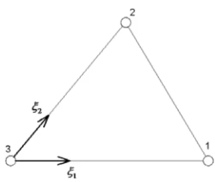
Figure 1: Triangular boundary element.
To solve equation 1 numerically, the boundary S is di-vided into sub-regions where displacements and tractions are approximated by known shape functions. In this work these sub-regions are of two types, finite boundary ele-ments (BEs) and infinite boundary eleele-ments (IBEs). The BEs employed are triangular, as shown in figure 1 with the local system of coordinates,ξ1ξ2, and the local node
numeration. The subsequent approximations are used for this BE:
uj =
3
k=1
Nkuk j, tj=
3
k=1
Nktk
j (2)
In expressions 2, the boundary values uj and tj are re-lated to the nodal values of the BE. The BEs have 3 nodes and for each node there are three components of displace-ment uk
j and traction tkj. The shape functions Nk used for these approximations are:
N1=ξ1, N 2
=ξ2, N 3
= 1−ξ1−ξ2 (3)
The same shape functions are used to approximate the boundary geometry:
xj =
3
k=1
Nkxkj (4)
where xk
j are the node coordinates. For IBEs, displace-ments and tractions are interpolated with the same func-tions:
uj = N p
k=1
Nkukj, tj= N p
k=1
Nktkj (5)
Each IBE has N pnodes and notN odas the BEs. The IBEs geometry, on the other hand, is approximated using special mapping functions, as discussed with more details in Section 3.
By substituting expressions 2 and 5 at equation 1, the
subsequent equation is obtained:
cij(y)uj(y) + NBE e=1 3 k=1
∆Tek ij ukj
+
+ NI BE
e=1 N p k ∆∞ Tek ijukj
= NBE e=1 3 k=1
∆Uek ijtkj
+
+ NI BE
e=1 N p k=1 ∆∞
Uijekt k j
(6)
NBE is the number of BEs andNIBE is the number of IBEs. For BEs:
∆Tijek=
γe
|J|NkTijdγe, ∆Uijek=
γe
|J|NkUijdγe
(7)
In equation 7 the global system of coordinates is trans-formed to the local one using the Jacobian |J| = 2A, whereAis the element area in the global system. On the other hand, for IBEs:
∆∞ Tek ij = γe |∞
J|NkT ijdγe,
∆∞ Uek ij = γe |∞
J|NkU
ijdγe (8)
Special mapping functions are used to calculate |∞
J|, as detailed in Section 3.
The integrals of equations 7 and 8 are calculated employ-ing standard BEM techniques. Non-semploy-ingular integrals are numerically evaluated using integration points. The sin-gular ones, on the other hand, are evaluated using the technique presented in reference [9]. In the end, the free termcij may be obtained by rigid body motions.
Writing equation 6 for all boundary nodes, as described in [10], one obtains the following system of equations:
∆T ·u= ∆U·t (9)
The ∆Tek
ij element contributions, including the free term
cij, are assembled to matrix ∆T and ∆Uek
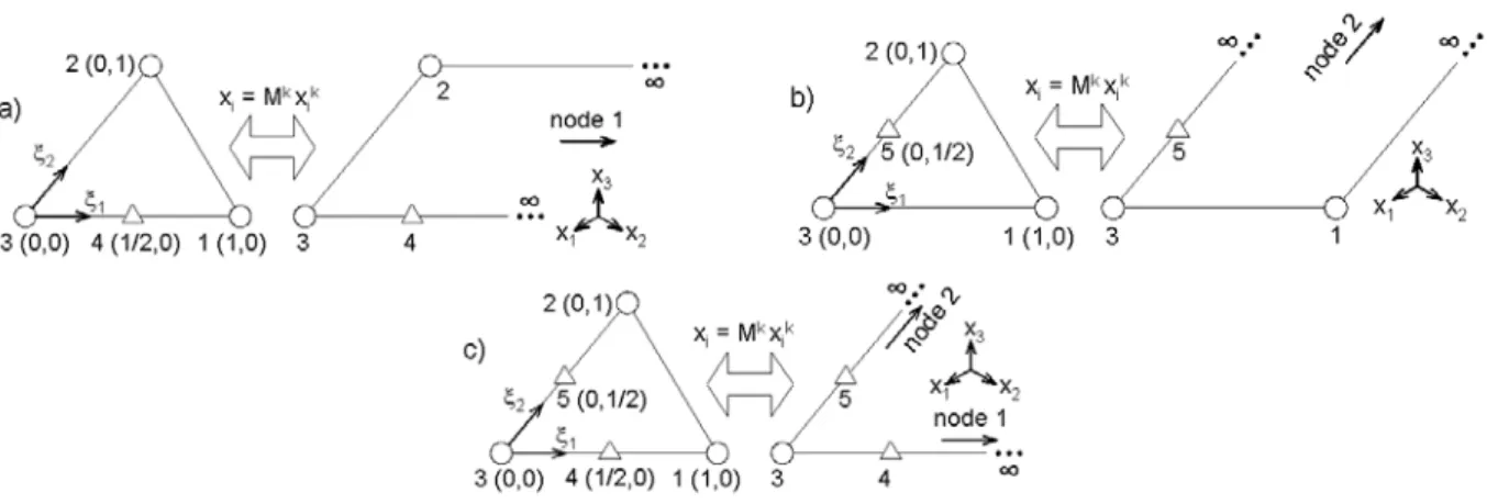
placed at a finite distance. Three types of mapping are considered, as illustrated in figure 2.
In the first type of mapping, as represented in Figure 2a, only directionξ1is mapped and node 1 is placed at
infini-ty. The IBE is represented in the local coordinate system on the left side, and in the global coordinate system on the right side. The global coordinates xi are related to the local ones using special mapping functions,Mk, and the nodal global coordinates,xk
i. Node 4 is created only to replace node 1 for the mapping and do not contribute with the integrals.
Figure 2b is analogous to Figure 2a, but in this case only direction ξ2 is mapped and node 2 is placed at infinity.
Therefore, node 5 is created to auxiliate the mapping. Finally, in Figure 2c both local directions are mapped and nodes 1 and 2 are placed at infinity. As a result, the auxiliary nodes 4 and 5 must be created to replace them in the mapping.
In this work, an auxiliary coordinate ¯ξi(ξi) is created in order to obtain the mapping functions. After analyzing some options and considering reference [11], the following function was chosen:
¯
ξi=
ξi 1−ξi
(10)
Using expression 10 and considering directionξ1mapped,
the following relation is obtained:
¯
ξ1(ξ1) =
ξ1
1−ξ1
(11)
and to map directionξ2:
¯
ξ2(ξ2) =
ξ2
1−ξ2
(12)
In the end, the mapping functions are obtained by sub-stituting the relations 11 and 12 in the shape functions 3 of the original BE. In such a way, to map only direc-tion ξ1 as illustrated in figure 2a, equation 11 must be
substituted in the shape functions 3. As a result, one obtains:
M14∞= ¯ξ1(ξ1) =
ξ1
1−ξ1
(13)
M2
1∞=ξ2 (14)
• Their sum must be equal to 1;
• The sum of their derivatives must be equal to zero;
• Any mapping function is equal to 1 on the corres-ponding node, and to zero on the other nodes;
• For nodes at infinity, mapping functions tent to−∞
or +∞;
The last item do not apply to function M2
1∞ because it
refers to a direction that is not mapped. For all other cases, it is demonstrable that the items are verified by the defined mapping functions. These functions are then employed to relate the local system of coordinates to the global one. In other words:
xi=M
4 1∞x
4
i +M
2 1∞x
2
i +M
3 1∞x
3
i (16)
After obtaining expression 16, the Jacobian used when only directionξ1is mapped may be calculated as follows:
|∞
J1|=
∂x1
∂ξ1
∂x2
∂ξ2
−∂x2 ∂ξ1
∂x1
∂ξ2
= 2A1 (1−ξ1)
2 (17)
whereA1is the area of triangle defined by nodes 2, 3 and
4 in the global system of coordinates.
The same steps are repeated to obtain the Jacobian for mapping only in theξ2direction. That is, by substituting
12 in the shape functions, one obtains:
M21∞=ξ1 (18)
M5
2∞= ¯ξ2(ξ2) =
ξ2
1−ξ2
(19)
M3
2∞= 1−ξ1−ξ¯2(ξ2) = 1−ξ1−
ξ2
1−ξ2
(20)
The symbol “2∞” is used to indicate that only direction
ξ2 is mapped. As a result, mapping function M21∞ is
equal to the original mapping function. These functions also satisfy the verifications suggested in reference [12], as presented before. Therefore, the global system is related to the local one as follows:
xi=M21∞x 1
i +M
5 2∞x
5
i +M
3 2∞x
3
Figure 2: Types of mapping.
and the Jacobian is:
|∞
J2|=
2A2
(1−ξ2)
2 (22)
where A2 refers to the area of the triangle defined by
nodes 1, 3 and 5 in the global system of coordinates.
Finally, to map directionsξ1 andξ2 both expressions 11
and 12 must be substituted at the shape functions. The result is:
M∞4 =
ξ1
1−ξ1
(23)
M5 ∞=
ξ2
1−ξ2
(24)
M∞3 = 1−
ξ1
1−ξ1
− ξ2
1−ξ2
(25)
The symbol “∞” is used to indicate that both directions are mapped. Once more the functions satisfy the verifi-cations and may be used to relate the local and global systems of equations, as follows:
xi=M
4 ∞x
4
i +M
5 ∞x
5
i +M
3 ∞x
3
i (26)
and the Jacobian becomes:
|∞
J3|=
2A3
(1−ξ1) 2
(1−ξ2)
2 (27)
where A3 is the area of the triangle defined by nodes 3,
4 and 5 in the global system.
4
Results
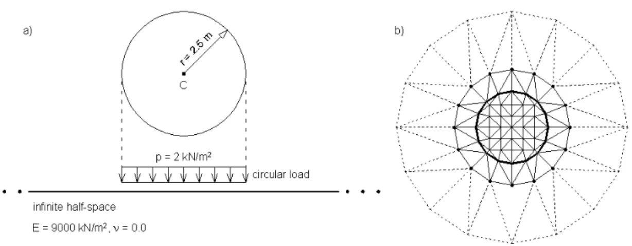
An example is now analyzed, as illustrated in Figure 3a, in order to test the presented formulation. A circular uniform load of 2 kN
m2
and with a radius of 2.5mis applied at the surface of an homogeneous half-space. The domain has an elasticity module of 9000 kN
m2
and a Poisson ratio of 0.0.
In reference [13] an analytical expression is presented for the vertical displacement at the central node of the loaded area, which is identified in figure 3a asC. This expression is:
d= 2rp
1−ν2
E (28)
where dis the vertical displacement at pointC,ris the radius of the circular load, p is the load value, ν is the Poisson ratio of the half space andEis its elasticity mo-dule. Substituting the values of figure 3a in expression 28, a displacement of 1.1111×10⁻³
mis obtained.
To simulate this problem a mesh with 57 nodes was ge-nerated, totalizing 96 BEs and 32 IBEs, as illustrated in figure 3b. The circle detached in the center corresponds to the loaded area, the dashed lines represent the IBEs and the rest of the mesh is composed by BEs. The points marked at the limits of the BE mesh are the ones that receive the influence of the IBEs. It is important to notice that no additional degrees of freedom are included by the presence of the IBEs, which is an advantage of this formulation.
Simulating this problem with the mesh of Figure 3b, a vertical displacement of 1.0850×10⁻³
m was obtained. This value agrees with the analytical solution, with an error of 2.4 %. In order to evaluate the influence of the IBEs, the example was simulated with the same BE mesh but no IBEs. A displacement of 1.0107×10⁻³
mwas than obtained, with the higher error of 9.0 % comparing to the analytical value.
The error increases when no IBEs are used because the domain is not well simulated as an infinite media. In order to improve this precision, more BEs and degrees of freedom need to be added at the mesh limits. In such a way, different meshes were tested and the results obtained are presented in Table 4.
Figure 3: a) Infinite domain problem; b) Mesh generated.
Nodes Displacement (m) Error (%) 57 1.0107×10⁻³
9.0 73 1.0391×10⁻³ 6
.5 89 1.0580×10⁻³
4.8 105 1.0699×10⁻³
3.7 121 1.0774×10⁻³
3.0 137 1.0820×10⁻³
2.6 153 1.0849×10⁻³
2.4
Table 1: Displacement calculation with BEs only.
results are achieved, however more degrees of freedom are needed. As may be observed, 153 nodes were needed for the BE mesh to equalize the precision of the first 57 node mesh, that was with IBEs. Comparing these two values it may be concluded that, in this example and maintaining the error of 2.4 %, the use of IBEs allows a mesh reduction of 63 %.
In tests with finer meshes at the central area, errors below 1 % were obtained. In such cases, comparing the number of nodes with and without IBEs, the mesh reduction is also very significant.
5
Conclusions and Future Work
This article presents a new mapped infinite boundary ele-ment (IBE) formulation, based on a triangular boundary element (BE) with linear shape functions. To obtain the mapping functions the local coordinate to be mapped is replaced by an auxiliary function, which was defined us-ing reference [11]. The resultus-ing functions are then used to relate the global system of equations with the local one, obtaining a Jacobian for each case.
The resulting IBE, when associated with a BE mesh, has the advantage of not increasing the original number of de-grees of freedom, as demonstrated in the example. The results obtained with the IBEs showed good agreement with an analytical solution, and the use of this
formula-tion promoted a mesh reducformula-tion of 63 %. The reducformula-tion calculated for other levels of precision was also very sig-nificant.
In future works, the authors intent to use IBEs together with BEs in problems involving infinite non-homogeneous half-spaces. The results here presented show that this formulation is adequate to this type of analysis.
References
[1] Karakus, M., Ozsan, A., Basarir, H., “Finite element analysis for the twin metro tunnel constructed in Ankara Clay, Turkey,” Bulletin of Engineering Ge-ology and the Environment, V66, pp. 71-79, 2007.
[2] Yin, L. Z., Yang, W., “Topology optimization for tunnel support in layered geological structures,” In-ternational Journal for Numerical Methods in Engi-neering, V47, pp. 1983-1996, 2000.
[3] Sadecka, L., “A finite/infinite element analysis of thick plate on a layered foundation,”Computers and Structures, V76, N5, pp. 603-610, 2000.
[4] Liu, D. S., Chiou, D. Y., Lin, C. H., “3D IEM formu-lation with an IEM/FEM coupling scheme for solv-ing elastostatic problems,”Advances in Engineering Software, V34, N6, pp. 309-320, 2003.
[5] Ribeiro, D. B., Almeida, V. S., Paiva, J. B., “Uma formula¸c˜ao alternativa para analisar a intera¸c˜ao solo n˜ao-homogˆeneo/ funda¸c˜ao/ superestrutura via acoplamento MEC-MEF,” Revista Sul-Americana de Engenharia Estrutural, V2, N2, pp. 27-46, 2005.
[7] Moser, W., Duenser, C., Beer, G., “Mapped infinite elements for three-dimensional multi-region bound-ary element analysis,”International Journal for Nu-merical Methods in Engineering, V61, pp. 317-328, 2004.
[8] Ribeiro, D. B., Beer, G., Souza, C. P. G., “Tun-nel excavation in rock mass with changing stiffness,”
EURO:TUN 2007 Computational Methods in Tun-nelling, Vienna, Austria, Vienna University of Tech-nology, 2007.
[9] Guiggiani, M., Gigante, A., “A general algorithm for multidimensional Cauchy principal value integrals in the boundary element method,”Journal of Applied Mechanics, V57, pp. 906-915, 1990.
[10] Brebbia, C. A., Dominguez, J.,Boundary Elements: An Introductory Course, Computational Mechanics Publications, London, 1992.
[11] Davis, P. J., Rabinowitz, P., Methods of numerical integration, Academic Press, New York, 1975.
[12] Bettess, P., Infinite elements, Penshaw Press, Sun-derland, UK, 1992.
[13] Burland, J.B., Broms, B.B., de Mello, V.F.B., “Be-havior of foundations and structures,” 9th