Quantifying pyroconvective injection heights using observations of fire energy: sensitivity of space-borne observations of carbon monoxide

(1)

ACPD

14, 22547–22585, 2014

Pyroconvection using fire energy

S. Gonzi et al.

Title Page

Abstract Introduction

Conclusions References

Tables Figures

◭ ◮

Back Close

Full Screen / Esc

Printer-friendly Version Interactive Discussion

Discussion

P

a

per

|

Discus

sion

P

a

per

|

Discussion

P

a

per

|

Discussion

P

a

per

|

Atmos. Chem. Phys. Discuss., 14, 22547–22585, 2014 www.atmos-chem-phys-discuss.net/14/22547/2014/ doi:10.5194/acpd-14-22547-2014

This discussion paper is/has been under review for the journal Atmospheric Chemistry and Physics (ACP). Please refer to the corresponding final paper in ACP if available.

Quantifying pyroconvective injection

heights using observations of fire energy:

sensitivity of space-borne observations of

carbon monoxide

S. Gonzi1, P. I. Palmer1, R. Paugam2, M. Wooster2, and M. N. Deeter3

1

School of GeoSciences, University of Edinburgh, Edinburgh, UK

2

Department of Geography, King’s College London, London, UK

3

National Center for Atmospheric Research NCAR, Boulder, CO, USA

Received: 31 July 2014 – Accepted: 6 August 2014 – Published: 3 September 2014 Correspondence to: S. Gonzi ([email protected])

(2)

ACPD

14, 22547–22585, 2014

S. Gonzi et al.

Title Page

Tables Figures

◭ ◮

Back Close

Full Screen / Esc

Discussion

P

a

per

|

Discus

sion

P

a

per

|

Discussion

P

a

per

|

Discussion

P

a

per

|

Abstract

We use observations of fire size and fire radiative power (FRP) from the NASA Moderate-Resolution Imaging Spectroradiometers (MODIS), together with a param-eterized plume rise model, to estimate biomass burning injection heights during 2006. We use these injection heights in the GEOS-Chem atmospheric chemistry transport

5

model to vertically distribute biomass burning emissions of carbon monoxide (CO) and to study the resulting atmospheric distribution. For 2006, we use over half a million FRP and fire size observations as input to the plume rise model. We find that con-vective heat fluxes and actual fire sizes typically lie in the range of 1–100 kW m−2and 0.001–100 ha, respectively, although in rare circumstances the convective heat flux can

10

exceed 500 kW m−2. The resulting injection heights have a skewed probability distribu-tion with approximately 80 % of injecdistribu-tions remaining within the local boundary layer (BL), with occasional injection height exceeding 8 km. We do not find a strong correla-tion between the FRP-inferred surface convective heat flux and the resulting injeccorrela-tion height, with environmental conditions often acting as a barrier to rapid vertical mixing

15

even where the convective heat flux and actual fire size are large. We also do not find a robust relationship between the underlying burnt vegetation type and the injec-tion height. We find that CO columns calculated using the MODIS-inferred injecinjec-tion height (MODIS-inj) are typically −9–+6 % different to the control calculation in which

emissions are emitted into the BL, with differences typically largest over the point of

20

emission. After applying MOPITT v5 scene-dependent averaging kernels we find that we are much less sensitive to our choice of injection height profile. The differences between the MOPITT and the model CO columns (max bias≈50 %), due largely to

uncertainties in emission inventories, are much larger than those introduced by the in-jection heights. We show that including a realistic diurnal variation in FRP (peaking in

25

(3)

ACPD

14, 22547–22585, 2014

S. Gonzi et al.

Title Page

Tables Figures

◭ ◮

Back Close

Full Screen / Esc

Discussion

P

a

per

|

Discus

sion

P

a

per

|

Discussion

P

a

per

|

Discussion

P

a

per

|

bias between model and MOPITT we find little impact on the resulting emission es-timates. Studying the role of pyroconvection in distributing gases and particles in the atmosphere using global MOPITT CO observations (or any current space-borne mea-surement of the atmosphere) is still associated with large errors, with the exception of a small subset of large fires and favourable environmental conditions, which will

con-5

sequently lead to a bias in any analysis on a global scale.

1 Introduction

Fire plays an important role in the evolution of the Earth system (Bowman et al., 2009). We focus on the influence of fires on determining the atmospheric distribution of car-bon monoxide (CO), a chemical tracer of incomplete combustion. In particular, we use

10

space-borne measurements of fire radiative power (FRP) and estimates of the fires surface area over which this radiative output is produced, to describe the enhanced vertical mixing due to intense surface heating to (a) understand the resulting atmo-spheric variation in CO, and (b) quantify the impact on surface flux estimates inferred from atmospheric measurements of CO.

15

Satellite observations have played a central role in understanding the spatial extent and seasonality of fires across different ecosystems (e.g., Cahoon Jr. et al., 1992; Bar-bosa et al., 1999; Carmona-Moreno et al., 2005; Csiszar et al., 2006; van der Werf et al., 2006; Giglio, 2007; Boschetti et al., 2010; Ichoku et al., 2012). There is a sub-stantial body of previous work on estimating biomass burning emissions of gases and

20

particles using space-borne instruments with varying levels of success (e.g., Duncan et al., 2003; Martin et al., 2003; Freitas et al., 2005; Ito and Penner, 2004; Kasis-chke and Penner, 2004; Edwards et al., 2006; Hodzic et al., 2007; Jordan et al., 2008; Kopacz et al., 2009; Liousse et al., 2010; Gonzi et al., 2011b; Fleming et al., 2012; Ross et al., 2013), largely reflecting heterogeneous sampling due to cloud and aerosol

25

(4)

ACPD

14, 22547–22585, 2014

S. Gonzi et al.

Title Page

Tables Figures

◭ ◮

Back Close

Full Screen / Esc

Discussion

P

a

per

|

Discus

sion

P

a

per

|

Discussion

P

a

per

|

Discussion

P

a

per

|

Recent studies have studied how injection heights can modify emitted gases and aerosols and downwind chemical composition (e.g., Palmer et al. (2013) and articles therein). Strictly speaking, pure pyroconvection is rare with most events triggered by storm systems that can result in unstable atmospheric conditions and enhance the vertical extent of the mixing due to the fire (e.g. Fromm et al., 2010; Dirksen et al.,

5

2009). The importance of vertical mixing due to some extent by surface heating from fire has been shown by a number of previous studies that have used models with and without a description of pyroconvection to interpret aircraft and satellite data (e.g., Freitas et al., 2010; Fisher et al., 2010; Sessions et al., 2011; Zhang et al., 2011; Pfister et al., 2011). Within these studies, pyroconvection is typically treated in an ad hoc

10

manner using a formulaic method of vertically redistributing surface emissions (e.g., Val Martin et al., 2012). FRP has been shown in small scale experiments to be related to rates of fuel combustion (Wooster et al., 2005) and to rates of key trace gas and aerosol emission (Freeborn et al., 2008). At the landscape scale previous work has shown that MODIS FRP measurements were related to the release rate of smoke

15

aerosols (Ichoku and Kaufman, 2005), and recently MODIS FRP has been used to map daily landscape-scale fuel consumption rates (Kaiser et al., 2012) and via the application of biome-specific emissions factors, the rates of release of various chemical species present in the smoke.

In the following section, we describe the FRP and active fire area estimates derived

20

(5)

ACPD

14, 22547–22585, 2014

S. Gonzi et al.

Title Page

Tables Figures

◭ ◮

Back Close

Full Screen / Esc

Discussion

P

a

per

|

Discus

sion

P

a

per

|

Discussion

P

a

per

|

Discussion

P

a

per

|

2 Data

2.1 MODIS fire observations

We use FRP values retrieved from MODIS on the Aqua and Terra satellites (Wooster et al., 2005; Ichoku et al., 2008). Both satellites are in a sun-synchronous, near-polar orbit. Terra and Aqua have an equatorial crossing time of 10:30 a.m. (10:30 p.m.) and

5

1:30 p.m. (1:30 a.m.) for their descending (ascending) nodes, respectively.

The FRP and Active Fire (AF) area for each fire are computed with the dual-band approach based on the bispectral algorithm of Dozier applied to the original MODIS calibrated Middle wave Infra Red (MIR) and Long Wave Infra Red (LWIR) radiance data (Dozier, 1981) stored in the active fire product (MOD14); a similar approach was

10

already used by Val Martin et al. (2012). For each granule, the hot spot detected by the fire detection algorithm of MODIS is assigned to a particular fire based on the analysis of clusters of spatially contiguous fire pixels. This is the same approach as previously applied with data from the BIRD Hot spot Recognition Sensor (Wooster et al., 2003; Zhukov et al., 2005). It is designed to minimize some of the problems of

15

the dual band method, for example those related to inter-channel spatial misregistration effects (Zhukov et al., 2005; Shephard and Edward, 2003). The average top of the atmosphere (TOA) radiances for each cluster are then corrected by the transmittance of the atmosphere in order to get the actual radiance emitted by the fire. The transmittance in each band is estimated from a precompiled lookup table based on the total amount

20

of column water (from ECMWF reanalysis) and the view angle of the sensor (Govaerts et al., 2010). Both corrected MIR and LWIR radiance are then subject to analysis using the “dualband” approach (Dozier, 1981), using the specific method taken by Zhukov et al. (2005). Outputs for each cluster are the size and the temperature of the equivalent black body which has the same thermal emission signal as the observed fire in the MIR

25

(6)

ACPD

14, 22547–22585, 2014

S. Gonzi et al.

Title Page

Tables Figures

◭ ◮

Back Close

Full Screen / Esc

Discussion

P

a

per

|

Discus

sion

P

a

per

|

Discussion

P

a

per

|

Discussion

P

a

per

|

Previous work has shown this method of FRP estimation introduced an uncertainty of around±10 % for fire temperature of 600–1600 K, with the advantage that the

temper-ature of the fire does not need to be known (Wooster et al., 2005, 2003). The MODIS instrument is less sensitive to wildfires with temperature<600 K, where gases emitted from smouldering is expected to be more substantial. We do not expect this high

tem-5

perature bias will compromise our method of describing the associated vertical mixing which is typically limited to the BL; as described below, in the absence of an FRP value we distribute emissions in the first few vertical model layers.

Figure 1 shows the MODIS derived distribution of half a million colocated FRP and active burnt area data during 2006. The measurement density is highest over equatorial

10

regions, with higher latitudes having less observations that reflect their seasonal cycle. We chose 2006 because FRP and fire size observations allows us to compare results with previous work (e.g., Gonzi et al., 2011a).

2.2 MOPITT column observations of CO

We use MOPITT v5 CO profile retrievals and the corresponding retrieval error

covari-15

ances and scene dependent averaging kernels for 2006 (Deeter, 2011). CO concen-trations are retrieved for ten pressure levels (surface, 900, 800, . . . 100 hPa) in the mul-tispectral thermal-IR/near-IR (TIR/IR) regions based on log-normal statistics and an optimal estimation method. We do not consider the TIR- and NIR-only products here. The a priori CO information in the MOPITT retrieval algorithm is calculated with the

20

global chemistry transport model MOZART (Horowitz et al., 2003) and meteorology in the retrieval algorithm is based on NCEP reanalysis data (Kalnay et al., 1996). The de-gree of freedom (DOF) for the multispectral TIR/IR retrievals is typically between 1.0– 2.2; in comparison, NIR- and TIR-only products have DOFs peaking at 0.1–1.0 and 0.5–1.5, respectively (Deeter et al., 2012). Past analyses show that these MOPITT CO

25

(7)

ACPD

14, 22547–22585, 2014

S. Gonzi et al.

Title Page

Tables Figures

◭ ◮

Back Close

Full Screen / Esc

Discussion

P

a

per

|

Discus

sion

P

a

per

|

Discussion

P

a

per

|

Discussion

P

a

per

|

three observations in a 1◦

×1◦grid cell for each day. We only use profile retrievals with

a DOF>1.3 and profiles for which the CO concentrations at 500 hPa are greater than 40 ppb (Gonzi et al., 2011a). This reduces the number of profiles considerably to ap-proximately five million observations during 2006. We find that using a more relaxed DOF criteria so that more observations are collected per gridbox (not shown) does not

5

signficantly affect our final analysis.

3 Models

3.1 Plume rise model

Pyroconvection is currently a sub-grid scale model process; resolving this process in a global model would involve prohibitive computational costs. Consequently, models

10

tend to parameterize this process if they include it at all. We use an established 1-D plume rise model (Freitas et al., 2006, 2010), embedded within the GEOS-Chem at-mospheric chemistry transport model described below, to describe the vertical mixing due to surface heating and consequently to redistribute surface emissions from the fire. The plume rise model estimates the injection height, defined as the level of

neu-15

tral buoyancy, by solving equations for the vertical plume velocity, plume temperature, condensation and evaporation (latent heat), accounting for wind shear. We use a pa-rameterization to conserve mass (Appendix A), which is an extension to the original code first published by (Freitas et al., 2006).

Initial surface boundary conditions in the plume rise model include MODIS derived

20

convective heat flux (kW m−2_{, defined below) and active burnt area (m}2_{), respectively,}

environmental temperature (K), relative humidity profile (%) and horizonal wind fields (m s−1). We drive the plume model using meteorological data from version 5 of the NASA Goddard Earth Observing System Model (GEOS-5) (Rienecker et al., 2008), ensuring consistency with the GEOS-Chem meteorology. For each MODIS derived

25

(8)

ACPD

14, 22547–22585, 2014

S. Gonzi et al.

Title Page

Tables Figures

◭ ◮

Back Close

Full Screen / Esc

Discussion

P

a

per

|

Discus

sion

P

a

per

|

Discussion

P

a

per

|

Discussion

P

a

per

|

role of atmospheric water vapour vs. water released from fuel combustion is still subject to debate (e.g., Penner et al., 1986; Potter, 2005; Trentmann et al., 2006, 2009; Cun-ningham and Reeder, 2009). We assume a fuel moisture of 10 %, calculated from the colocated GEOS-5 relative humidity profile, which we add to the existing atmospheric levels. We further assume that the initial plume temperature equals the environmental

5

temperature. The biggest source of moisture varation is from the atmosphere, which is updated with each time step during the fire as the plume temperature changes. Estimates of convective heat flux are also uncertain. Here, we use flux estimates in-ferred from FRP observations, assuming an underlying relationship between the two variables. Fire energy can broadly speaking be separated into three components:

con-10

duction, radiation and convection. The contribution from these sources to the total fire energy is uncertain, but it can be assumed that convection is as important as radia-tive energy (Anderson et al., 2010; Butler, 2010; Finney et al., 2012; Frankman et al., 2012). The maximum radiative heat yield that is typically measured by MODIS is about 20 % (Wooster et al., 2005) of the total heat whereas the maximum heat yield that can

15

theoretically be liberated by a fire is between 20 % and 60 % (Ferguson et al., 2000). We assume that heat loss by conduction is relatively small compared to losses by the combined effect of radiation and convection. We assume an average heat loss of 15 % for radiation, 10 % for conduction, and 75 % due to convection (H_F, kW m−2). The loss by convection is then given asHF =5×FRPA , where A (m

2

) denotes the actual burnt

20

fire size. We acknowledge here that this relation is probably the upper limit and will not hold true for every location and fire type around the globe, but it is a reasonable mean estimate based on current knowledge.

3.2 The GEOS-Chem atmospheric chemistry model

We use GEOS-Chem version 9-01-01 (www.geos-chem.org) as the forward model that

25

(9)

ACPD

14, 22547–22585, 2014

S. Gonzi et al.

Title Page

Tables Figures

◭ ◮

Back Close

Full Screen / Esc

Discussion

P

a

per

|

Discus

sion

P

a

per

|

Discussion

P

a

per

|

Discussion

P

a

per

|

a horizontal resolution of 2◦

×2.5◦, with 47 sigma levels that span the surface to 0.01 hPa

of which 30 levels are within the troposphere. The 3-D meteorological data is updated every six hours, and heights of the BL and tropopause are updated every three hours. We use monthly mean emission inventories for fossil fuel (Olivier and Berdowski, 2001; Streets et al., 2006), biofuel (Yevich and Logan, 2003), and biomass burning

5

(van der Werf et al., 2010), and from the oxidation of volatile organic compounds (Dun-can et al., 2007). Atmospheric oxidation by OH is the main atmospheric loss of CO, resulting in a lifetime of weeks to months depending on latitude and season. We use monthly 3-D fields of the OH sink precomputed from a full chemistry version of the model. Fixing the OH sink e_ffectively allows us to linearly decompose the

contribu-10

tions of CO from source types and/or geographical regions. Figure 1 shows the eight geographical regions we study, reflecting the location of burning. For each region we track emissions from biomass burning and combined emissions from fossil fuel and biofuel combustion. We also track the combined contribution of CO from the oxidation of methane, isoprene, monoterpenes, methanol, and acetone. A more detailed

descrip-15

tion of this model can be found elsewhere (Duncan et al., 2007; Gonzi et al., 2011a). We sample the model at the time and location of MODIS and MOPITT measurements. Below, where we discuss model bias we define percentage bias as

Bias=100× COM−COX

max(CO_M, CO_X), (1)

20

where CO_M denotes the model and CO_Xdenotes either the model control CO_Cor the observed atmospheric measurement COO.

For the control run (and the default setting of GEOS-Chem), we release biomass burning emissions within the BL in which there are approximately 15 levels from the surface to 2.5 km. For the sensitivity runs using FRP to define the injection height

25

(10)

ACPD

14, 22547–22585, 2014

S. Gonzi et al.

Title Page

Tables Figures

◭ ◮

Back Close

Full Screen / Esc

Discussion

P

a

per

|

Discus

sion

P

a

per

|

Discussion

P

a

per

|

Discussion

P

a

per

|

hour window, determined by the GEOS-5 analyses, determines the surface convective heat flux boundary conditions. In the typical case of more than one FRP observation falling in a grid square during this time window, we create an injection height profile for each associated convective heat flux: equally distributing emitted mass from the surface to the injection height or from the local BL to the injection height whenever the

5

injection height is larger than the BL. We then calculate an effective injection height by calculating a sum of individual profiles weighted by their respective fractional actual area burnt within that grid box. This fractional scaling ensures that the final effective profile conserves mass. If there are no FRP observations in a model grid box for a par-ticular time but emissions are non-zero we distribute emissions within the local BL.

10

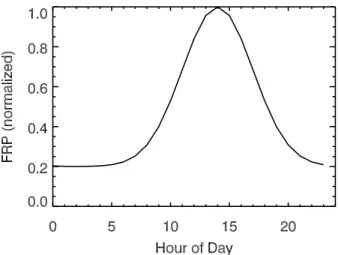
We also consider the sensitivity of our results to imposing a diurnal cycle on FRP, following analysis of similar data as a function of land cover type over Africa using the Spinning Enhanced Visible and Infrared Imager (SEVIRI) (Roberts et al., 2009). Figure 2 shows that the mean diurnal cycle peaks during early afternoon, consistent with previous analysis of data from the GOES WF_ABBA (Geostationary Operational

15

Environment Satellite Wildfire Automated Biomass Burning Algorithm) active fire ob-servations that show early afternoon peaks valid for the entire globe (Giglio, 2007; Mu et al., 2011). We use this mean diurnal profile to effectively relate observations taken at discrete times to the rest of the day, acknowledging this is a crude but reasonable assumption.

20

3.3 The maximum a posteriori (MAP) inverse model

We briefly describe our inverse model approach here that has been discussed at length elsewhere (Gonzi et al., 2011a). We sample the model along the MOPITT orbit by ap-plying scene-dependent averaging kernels from MOPITT and follow an optimal estima-tion method in order to fit the model 3-D CO concentraestima-tions to the observaestima-tions.

25

(11)

ACPD

14, 22547–22585, 2014

S. Gonzi et al.

Title Page

Tables Figures

◭ ◮

Back Close

Full Screen / Esc

Discussion

P

a

per

|

Discus

sion

P

a

per

|

Discussion

P

a

per

|

Discussion

P

a

per

|

estimate lumped emissions from biomass burning, fossil fuel and biofuel emissions on a quarterly basis (JFM, AMJ, JAS, and OND). We assume a priori uncertainties of 50 % for incomplete combustion emissions and 25 % for the chemical oxidation source, following previous work (Gonzi and Palmer, 2010). For measurement errors, we include the local scene-dependent retrieval error from MOPITT to the final total error in

log-5

space. We also include a 25 % uncertainty associated with the combined forward model and representation errors. The MAP algorithm described in a log-measurement space typically converges after a few iterations (Gonzi et al., 2011b).

4 Results

4.1 Convective heat fluxes, burned area, and injection heights for 2006

10

Figure 1 shows for 2006 the annual mean values for convection heat flux (kW m−2) inferred from MODIS FRP measurements, and the corresponding actual burnt areas (hectares) used to determine the local pyroconvection injection height. The geograph-ical variation of measurements available to calculate injection height reflects the fquency of fires and the magnitude of associated FRP derived heat flux, which is

re-15

lated to the fire regime of an area, and to the intensity of the energy emission from those fires. In general, the mean (not shown) and median values of the fire products are similar, suggesting there is little skewness in the distribution of FRP, although we acknowledge that the highest values are typically a factor of 5–10 higher than the mean value and that the median is in general the more robust statistic for this parameter.

Fig-20

ure 3 shows the corresponding global monthly box-and-whisker plots for convective heat flux and actual burnt area, respectively. The bulk of convective heat flux values are typically in the range 1–100 kW m−2and burnt areas typically lie in the range 0.1– 10 ha. On occasion, active burnt area estimates can exceed 500 ha but these represent only a small percentage of the data.

(12)

ACPD

14, 22547–22585, 2014

S. Gonzi et al.

Title Page

Tables Figures

◭ ◮

Back Close

Full Screen / Esc

Discussion

P

a

per

|

Discus

sion

P

a

per

|

Discussion

P

a

per

|

Discussion

P

a

per

|

Figure 1 shows the corresponding injection heights determined by the plume rise model. These data shows that the FRP-derived estimates of convective heat flux and actual fire size are insufficient by themselves to determine the injection height. This disagrees with field experiment data (Lavoué et al., 2000), but these were small-scale experiments with final injection heights that did not consider atmospheric stability

con-5

straints.

4.1.1 Sensitivity of injection heights to environmental parameters

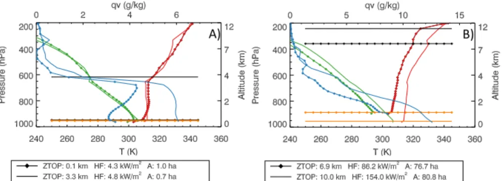
Figure 4 shows two examples where values for MODIS FRP and/or actual fire size are similar but the analyzed meteorology for atmospheric temperature and specific humid-ity are different, resulting in different injection heights. Figure 4a show two instances

10

where HF and A have similar values but the lower injection height (0.1 km vs. 3.3 km) is associated with a more stable atmosphere as determined by the negative gradi-ent in potgradi-ential temperature and higher specific humidity. This serves as an example where even modest changes in potential temperature can result in large changes to the model injection height. Figure 4b shows a contrasting example where there is clearly

15

a positive gradient in potential temperature, indicative of a stable, stratified atmosphere, but the injection heights are much larger than the corresponding local BL heights. For these two cases values of HF and A are very large with the only difference being that the higher injection height (10 km vs. 6.9 km) having almost twice the HF. These two examples highlight the two limits that determine injection height: (1) small fires that rely

20

on unstable environmental conditions to penetrate the free troposphere and (2) large fires (defined here as having high FRP and large active fire area) that can overcome locally stable environmental conditions to penetrate into the free troposphere. There are of course a continuum of possible combinations of variables between these two limits that determine the final injection height.

25

(13)

ACPD

14, 22547–22585, 2014

S. Gonzi et al.

Title Page

Tables Figures

◭ ◮

Back Close

Full Screen / Esc

Discussion

P

a

per

|

Discus

sion

P

a

per

|

Discussion

P

a

per

|

Discussion

P

a

per

|

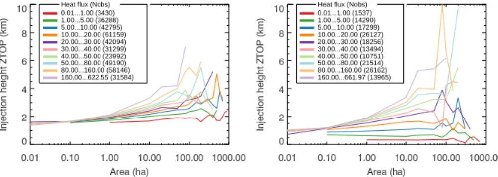
we reach areas>80 hectares. We also find a similar relationship between the injec-tion height and heat flux. This supports the idea that above a certain threshold of fire energy released the buoyancy induced by the fire can overcome locally stable mete-orological conditions. Figure 5 also shows that the metemete-orological stability conditions play a progressively important role as the fire area and heat flux increases.

5

Previous work derived a plume height climatology based on a compilation of MODIS FRP and actual burnt area (Val Martin et al., 2012). These data were used to test the ability of a 1-D plume rise model in predicting the injection heights inferred from the Multi-angle Imaging SpectroRadiometer space-borne instrument (Diner et al., 2010) during the 2002, 2006 and 2007 North American burning seasons. They found that the

10

plume rise model typically underpredicts the injection heights into the free troposphere due to the uncertain nature of input paramaters as FRP, fire size, and environmental meteorological conditions. They argue that a pre-compiled classification of injection heights as a function of parameters described in a look-up table may be an e_fficient approach to including injection heights in global models. While we agree that there

15

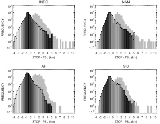
is an urgent need for a predictive capability for plume rise, we believe that finding a robust relationship with injection height may well be as uncertain as using the plume rise model itself. We find that the biggest uncertainties is identifying the stability of the overlying atmosphere given the coarse meteorological information from global models. Figure 6 shows that the normalized frequency distribution of injection heights over

20

key burning regions are consistent, with differences only in the extent of the tails. This suggests that in almost all biomass burning regions smaller and less intense fires dom-inate with di_fferences due mainly to the number of extreme fires, and how extreme they are. For example one might expect Canada to have a larger number of high intensity, large active fire area fires compared to Russia since we know Canada has a greater

25

proportion of Crown fires than surface fires compared to Russia (e.g. Wooster and Zhang, 2004). For brevity we focus on a few regions. The median injection height for all regions is≃1.5 km, with the highest injection heights of>6 km over Indonesia, Africa,

(14)

ACPD

14, 22547–22585, 2014

S. Gonzi et al.

Title Page

Tables Figures

◭ ◮

Back Close

Full Screen / Esc

Discussion

P

a

per

|

Discus

sion

P

a

per

|

Discussion

P

a

per

|

Discussion

P

a

per

|

account uncertainty of the BL value) from this we find that typically 20 % of fires are injected above the BL consistent with bulk statistics reported in previous work (Val Mar-tin et al., 2010). If we increase the free troposphere threshold to the local BL+500 m we find that the fraction of fire reaching the free troposphere drops to 10–20 %; where Africa, Asia and North America is most affected suggesting these fires only just reach

5

the free troposphere.

Val Martin et al. (2010) studied 584 MISR plumes over North America for the years 2002, 2006–2007 and their scaled-FRP/FRPx10 set-up found that 16–35 % (500– 250 m BL uncertainty) reached the free troposphere compared to 24–48 % observed by MISR. We find that over North America during 2006, 14–22 % (500–250 m BL

un-10

certainty) reach the free tropopshere. While the percentage of model plumes reaching the free troposphere over North America is similar to MISR they are not necessary the same group of plumes (Val Martin et al., 2010).

We use land cover classifications from AVHRR and MODIS observations (Hansen et al., 2000; Friedl et al., 2002) to investigate the relationship between the land cover

15

(savannah, agriculture, peat, tropical and extratropical forest), FRP of fires and the re-sulting injection heights. We find that agricultural fires have a median FRP of 20 MW and are typically lower than over the other four biomes that have median values of 30 MW (not shown). The corresponding injection height mean statistics are similar for all vegetation types with the exception of agricultural for which heights<5 km.

Agricul-20

tural fires are small and typically low intensity, resulting in what would be expected to be low FRP for the fires when compared, for example, to many other types of fire. We also found no evidence to support that injection heights for extratropical forests were higher than from other biomes.

4.2 The sensitivity of atmospheric CO to pyroconvection

25

(15)

dis-ACPD

14, 22547–22585, 2014

S. Gonzi et al.

Title Page

Tables Figures

◭ ◮

Back Close

Full Screen / Esc

Discussion

P

a

per

|

Discus

sion

P

a

per

|

Discussion

P

a

per

|

Discussion

P

a

per

|

tributions. We then compare this model output to see whether it improves agreement with available data relative to the model that assumes an injection height that is limited to the BL.

To help evaluate our model during 2006, we use exclusively space-borne observa-tions of CO from the v5 MOPITT CO profile retrievals (Deeter et al., 2013). The two

5

major airborne campaigns MOZAIC (Marenco et al., 1998) and INTEX-B (Arellano Jr. et al., 2007) that measured CO during this period are not ideal for studying biomass burning. Previous work has showed that MOPITT data can be used to estimate emis-sions of CO from biomass burning (e.g., Pfister et al., 2005; Arellano Jr. et al., 2006; Chevallier et al., 2008; Kopacz et al., 2009; Gonzi et al., 2011a, b) but there still

ex-10

ists large uncertainties associated with the magnitude and timing of these emissions, reflecting model errors but also the coverage and uncertainties associated with MO-PITT. As discussed in Sect. 3.2 we sample the model at the time and location of each MOPITT scene and convolve the resulting profile in log space with scene-specific av-eraging kernels.

15

Figure 7 shows that the model using the injection height estimate inferred from MODIS as a daily mean value has the largest differences (−5–+2 %), relative to the

control, over and downwind of central and southern Africa. Including our diurnal varia-tion of FRP (Fig. 2) increases the magnitude and spatial extent of the differences over and downwind of Africa and also introduces differences over Siberia and to a lesser

20

extent over Southeast Asia and Australia. A cross section plot along the latitudes vs. altitude (Fig. 7) shows that the largest averaged monthly negative bias occurs in the BL at≈ −12◦ latitude, corresponding to the largest negative bias in the total columns.

If we then convolve the model profiles with scene-dependent MOPITT averaging ker-nels these differences (not shown) are substantial reduced to<±2 %. We find that the

25

differences (±50 %) between model values as would be observed by MOPITT space

(16)

ACPD

14, 22547–22585, 2014

S. Gonzi et al.

Title Page

Tables Figures

◭ ◮

Back Close

Full Screen / Esc

Discussion

P

a

per

|

Discus

sion

P

a

per

|

Discussion

P

a

per

|

Discussion

P

a

per

|

order of magnitude larger than the model response convolved with MOPITT averaging kernels to different prescriptions of injection height. Previous work used the GEOS-Chem model to infer CO emissions from MOPITT v5 CO profiles between June and August 2006 (Jiang et al., 2012). They found that posterior emission estimates were sensitive to the pressure level used: GEOS-Chem over(under)-estimates CO at lower

5

(middle and upper) levels.

Figure 8 shows an example of model and MOPITT CO profiles over Siberian forest fires. The model CO mixing ratio with and without MODIS-inferred injection height using our diurnal distribution is 30–80 ppb in the lower troposphere. After we relate model CO concentrations to CO columns which are observed by MOPITT using the relevant

10

averaging kernel (Fig. 8) the di_fference between the two models reduces to<10 ppb. We find the resulting model profile overestimates (underestimates) CO at the surface (in the free troposphere), relative to MOPITT. The corresponding column amounts are 3.3×1018molec cm−2for MOPITT and 2.4×1018molec cm−2(2.3×1018 molec cm−2)

for the model with (without) scene-dependent injection height. For this example, it is

15

clear that the model minus MOPITT bias of 27 % is much larger than the 5 % difference between the two model calculations. We find similar instances over the other burning loci around the world. We show this example profile because it corresponds to the time and location of the largest bias (≈5 %) between model w/wo injection height over the

region SIB (Fig. 7). MOPITT profiles have generally finer vertical resolution.

20

For the above calculations we have assumed that material is distributed uniformally from the surface to the prescribed injection height. We consider two alternative for-mulations. First, we take into account that the majority of surface fires will typically be

<2◦×2.5◦ (≈62 500 km2), and acknowledge that only the most intense of these will

play a substantial role in determining atmospheric composition. We select the fires

25

(17)

ACPD

14, 22547–22585, 2014

S. Gonzi et al.

Title Page

Tables Figures

◭ ◮

Back Close

Full Screen / Esc

Discussion

P

a

per

|

Discus

sion

P

a

per

|

Discussion

P

a

per

|

Discussion

P

a

per

|

by eddies in the mixing processes will deposit emissions at heights below the highest value. To address this we incorporate a normalized parabolic injection height profile with a half-width maximum of 1 km such that the profile integrates to unity (InJS2). For both sensitivity runs we produce a corresponding control run that can be used to as-sess the importance of the parameter being perturbed. We find that the maximum total

5

column bias in Fig. 7 is about a factor of two larger for InjS1 than for InjS2 (not shown), although the spatial distribution of the bias is the same, as expected, but is still small compared to the model minus MOPITT differences.

We have reported that MOPITT averaging kernels are often broader than the ver-tical sensitivity necessary to distinguish between different prescribed vertical injection

10

heights due to surface heating. This is reflected in more detailed analyses involve MAP algorithms for which we find only small adjustments to posterior emissions compared to differences due to emissions that have been published previously (e.g., Gonzi et al., 2011a). We therefore do not discuss this any further.

5 Concluding remarks

15

We presented the first global, annual study of space-borne observations of fire radia-tive power and fire size to study the resulting injection heights. We used MODIS FRP and fire size observations for 2006 to improve understanding their relationship and the resulting injection height by embedding a 1-D plume-rise model into a global 3-D chem-istry transport model. We did not find a robust relationship between FRP, fire size and

20

injection height, and suggest that any e_ffort to find one may be as uncertain as using these data as for scene-specific initial conditions for a 1-D plume-rise model.

We demonstrated using the plume rise model that different prescriptions of injection height do have an impact on atmospheric CO concentrations over intense fires. In gen-eral, model bias against MOPITT can be as large as 50 %, which dwarves any realistic

25

(18)

exam-ACPD

14, 22547–22585, 2014

S. Gonzi et al.

Title Page

Tables Figures

◭ ◮

Back Close

Full Screen / Esc

Discussion

P

a

per

|

Discus

sion

P

a

per

|

Discussion

P

a

per

|

Discussion

P

a

per

|

ples over large fires where MOPITT can differentiate between different prescriptions of vertical transport of CO emissions. As a consequence we cannot quantify the impact of injection heights on the inference of CO emissions from MOPITT CO profile data via an inverse model. The major implication from this result is that outside of detailed case studies, use of MOPITT to quantify biomass burning emissions is biased towards

5

the very largest fires that can perturb substantial sections of the observed atmospheric column.

Space borne observations of FRP, fire area and other land-surface properties to-gether with atmospheric concentration measurement remain our best constraints for biomass burning emissions and associated vertical transport. More effective use of the

10

land-surface properties used in this study may require assimilation with a model that explicitly includes the observed parameters.

A new space-borne mission that retrieves biomass burning trace gases and associ-ated land-surface properties would be required to address some of the gaps in current understanding. Previous analysis of the atmospheric signature from biomass burning

15

using space-borne data has focused on CO using thermal IR sensors such as MO-PITT with greatest sensitivity in the free troposphere, or short-lived trace gases such as formaldehyde measured by UV/Vis sensors that require a detailed knowledge of at-mospheric chemistry (e.g., Gonzi et al., 2011b). The ideal mission would have a vertical resolution<1 km in the lower and free troposphere and a ground-pixel size of 1 km or

20

less. To achieve this a combined nadir/limb viewing instrument that measures thermal and short-wave IR wavelength may be required but integrating these data bring their own challenges (e.g., Gonzi and Palmer, 2010).

Appendix

The plume rise model variables are solved on a vertical grid comprising 200 levels in

25

(19)

ACPD

14, 22547–22585, 2014

S. Gonzi et al.

Title Page Abstract Introduction Conclusions References Tables Figures ◭ ◮ ◭ ◮ Back Close

Full Screen / Esc

Printer-friendly Version Interactive Discussion Discussion P a per | Discus sion P a per | Discussion P a per | Discussion P a per |

variableζ (Paugam et al., 2010).

∂w

∂t +w

∂w

∂z =

1

1+γgB−ǫw

2

(A1a)

∂T

∂t +w

∂T

∂z =−w

g

cp−

ǫw(T−T¯)+∂T

∂tmicro (A1b)

∂ζ

∂t =

∂wζ

∂z +wζ(ǫ−δ) (A1c)

∂φ

∂t +w

∂φ

∂z =−ǫw(φ−φe) (A1d)

5

ζ=ρR2 (A1e)

ǫ=max

0,C_ǫ B

w2

+C_ǫ1

w

du

dz (A1f)

δ=max

0,C_δ B

w2

+C_δC_ǫ1

w

du

dz, (A1g)

wherewdenotes vertical plume velocity (m s−1_),_T _{(K) is the plume temperature,}_T e(K) 10

is the environmental temperature,B(kg) is the buoyancy (gB),g(m s−2) gravitational constant,γ(unitless) scaling factor,c_p(J kg−1K−1) specific heat for constant pressure,

ζ mass (kg m−1

),ǫ(1 s−1

) andδ (1 s−1

) denote entrainment and detrainment, respec-tively, whereC_ǫ (–) and C_δ (–) are empirical, unitless scaling factors (Pergaud et al., 2009). The subscriptmicrotakes into account: evaporation, condensation, rain, ice with

15

respect to the saturation water mass mixing ratio.

The initial boundary conditions rely on GEOS-5 temperatures, relative humidity (available water), and wind fields. The actual area size and convective heat flux, re-spectively is based on MODIS derived observations (see main text). As we mentioned in the main text we calculate the available water (g m−2) from the fuel by a simple

for-20

(20)

ACPD

14, 22547–22585, 2014

S. Gonzi et al.

Title Page

Tables Figures

◭ ◮

Back Close

Full Screen / Esc

Discussion

P

a

per

|

Discus

sion

P

a

per

|

Discussion

P

a

per

|

Discussion

P

a

per

|

box:

water=Hf×

dt

H ×(0.5+fmoist)

0.55 ×1000, (A2)

whereHf is the convective heat flux (W m− 2

), H is the fuel its heat storage capacity (J kg−1), dt is the time step in (s), and fmoist is the moisture content of the fuel (–). 5

We assumefmoist has a ratio of 10 %. The factor 0.5 in the equation assumes 0.5 kg

is being emitted as water per 1 kg fuel burnt. ForH we choose a value of 19 MJ kg−1

representing typical fuel vegetation characteristics.

Acknowledgements. We thank Saulo Freitas (INPE/CPTEC) for useful discussions regarding

the plume rise model code. This work was supported by the UK Natural Environment Research

10

Council grant NE/E01819X/1. PIP gratefully acknowledges his Royal Society Wolfson Research Merit Award.

References

Anderson, W. R., Catchpole, E. A., and Butler, B. W.: Convective heat transfer in fire spread through fine fuel beds, Int. J. Wildland Fire, 9, 284–298, 2010. 22554

15

Arellano Jr., A. F., Kasibhatla, P. S., Giglio, L., van der Werf, G. R., Randerson, J. T., and Collatz, G. J.: Time-dependent inversion estimates of global biomass-burning CO emissions using Measurement of Pollution in the Troposphere (MOPITT) measurements, J. Geophys. Res., 111, D09303, doi:10.1029/2005JD006613, 2006. 22561

Arellano Jr., A. F., Raeder, K., Anderson, J. L., Hess, P. G., Emmons, L. K., Edwards, D. P.,

Pfis-20

ter, G. G., Campos, T. L., and Sachse, G. W.: Evaluating model performance of an ensemble-based chemical data assimilation system during INTEX-B field mission, Atmos. Chem. Phys., 7, 5695–5710, doi:10.5194/acp-7-5695-2007, 2007. 22561

Barbosa, P. M., Stroppiana, D., and Gregoire, J.-M.: An assessment of vegetation fire in Africa (1981–1991): burned areas, burned biomass, and atmospheric emissions, Global

Bio-25

(21)

ACPD

14, 22547–22585, 2014

S. Gonzi et al.

Title Page

Tables Figures

◭ ◮

Back Close

Full Screen / Esc

Discussion

P

a

per

|

Discus

sion

P

a

per

|

Discussion

P

a

per

|

Discussion

P

a

per

|

Boschetti, L., Roy, D. P., Justice, C. O., and Giglio, L.: An assessment of vegetation fire in Africa (1981–1991): burned areas, burned biomass, and atmospheric emissions, Int. J. Wildland Fire, 19, 705–709, 2010. 22549

Bowman, D. M. J. S., Balch, J. K, Artaxo, P., Bond, W. J., Carlson, J. M., Cochrane, M. A., D’Antonio, C. M., DeFries, R. S., Doyle, J. C., Harrison, S. P., Johnston, F. H., Keeley, J. E.,

5

Krawchuk, M. A., Kull, C. A., Marstona, J. B., Moritz, M. A., Prentice, I. C., Roos, C. I., Scott, A. C., Swetnam, T. W., van der Werf, G. R., and Pyne, S. J.: Fire in the Earth System, Science, 324, 481–484, 2009. 22549

Butler, B. W.: Characterization of convective heating in full scale wildland fires, in: International Conference on Forest Fire Research, edited by: Viegas, D. X., 15–18 November 2010,

Coim-10

bra, Portugal, 2010. 22554

Cahoon Jr., D., Stocks, B., Levine III, J., W. C., and O’Neill, K.: Seasonal distribution of African savanna fires, Nature, 359, 812–815, 1992. 22549

Carmona-Moreno, C., Belward, A., Malingreau, J., Hartley, A., Garcia-Algere, M., Antonovskiy, M., Buchshtaber, V., and Pivovarov, V.: Characterizing interannual variations in global fire

15

calendar using data from Earth observing satellites, Glob. Change Biol., 11, 1537–1555, 2005. 22549

Chevallier, F., Fortems, A., Bousquet, P., Pison, I., Szopa, S., Devaux, M., and Hauglus-taine, D. A.: African CO emissions between years 2000 and 2006 as estimated from MOPITT observations, Biogeosciences, 6, 103–111, doi:10.5194/bg-6-103-2009, 2009. 22561

20

Csiszar, I. A., Morisette, J. T., and Giglio, L.: Validation of active fire detection from moderate-resolution satellite sensors: the MODIS example in northern Eurasia, IEEE T. Geosci. Rem. Sens., 44, 1757–1764, 2006. 22549

Cunningham, P. and Reeder, M. J.: Severe convective storms initiated by intense wildfires: numerical simulations of pyro-convection and pyro-tornadogenesis, Geophys. Res. Lett., 36,

25

L12812, doi:10.1029/2009GL039262, 2009. 22554

Deeter, M. N.: MOPITT Measurements of Pollution in the Troposphere, Version 5 Prod-uct User’s Guide, Tech. rep., https://www2.acd.ucar.edu/sites/default/files/mopitt/v5_users_ guide_beta.pdf, last access: 31 August 2011. 22552

Deeter, M. N., Worden, H. M., Edwards, D. P., Gille, J. C., and Andrews, A. E.: Evaluation of

MO-30

(22)

ACPD

14, 22547–22585, 2014

S. Gonzi et al.

Title Page

Tables Figures

◭ ◮

Back Close

Full Screen / Esc

Discussion

P

a

per

|

Discus

sion

P

a

per

|

Discussion

P

a

per

|

Discussion

P

a

per

|

Deeter, M. N., Martinez-Alonso, S., Edwards, D. P., Emmons, L. K., Gille, J. C., Worden, H. M., Pittman, J. V., Daube, B. C., and Wofsy, S. C.: Validation of MOPITT version 5 thermal-infrared, near-thermal-infrared, and multispectral carbon monoxide profile retrievals for 2000–2011, J. Geophys. Res., 118, 6710–6725, doi:10.1002/jgrd.50272, 2013. 22552, 22561

Diner, D., Ackerman, T., Braverman, A., Bruegge, C., Chopping, M., Clothiaux, E., Davies, R.,

5

Girolamo, L. D., Kahn, R., Knyazikhin, Y., Liu, Y., Marchand, R., Martonchik, J., Muller, J., Nolin, A., Pinty, B., Verstraete, M., Wu, D., Garay, M., Kalashnikova, O., Davis, A., Davis, E., and Chipman, R.: Ten years of MISR observations from Terra: looking back, ahead, and in between, Proc. IEEE Int. Geosci. Remote Sens. Symp., pp. 1297–1299, 2010. 22559 Dirksen, R. J., Boersma, K. F., de Laat, P., Stammes, J., van der Werf, G., Martin, M. V., and

10

Kelder, H. M.: An aerosol boomerang: rapid around-the-world transport of smoke from the December 2006 Australian forest fires observed from space, J. Geophys. Res., 114, D21201, doi:10.1029/2009JD012360, 2009. 22550

Dozier, J.: A method for satellite identification of surface temperature fields of subpixel resolu-tion, Remote Sens. Environ., 11, 221–229, 1981. 22551

15

Duncan, B. N., Martin, R. V., Staudt, A. C., Yevich, R., and Logan, J. A.: Interannual and sea-sonal variability of biomass burning emissions constrained by satellite observations, J. Geo-phys. Res., 108, 4040, doi:10.1029/2002JD002378, 2003. 22549

Duncan, B. N., Logan, J. A., Bey, I., Megretskaia, I. A., Yantosca, R. M., Novelli, P. C., Jones, N. B., and Rinsland, C. P.: Global budget of CO, 1988–1997: source estimates and validation

20

with a global model, J. Geophys. Res., 112, D22301, doi:10.1029/2007JD008459, 2007. 22555

Edwards, D. P., Emmons, L. K., Gille, J. C., Chu, A., Attié, J.-L., Giglio, L., Wood, S. W., Hay-wood, J., Deeter, M. N., Massie, S. T., Ziskin, D. C., and Drummond, J. R.: Satellite-observed pollution from Southern Hemisphere biomass burning, J. Geophys. Res., 111, D14312,

25

doi:10.1029/2005JD006655, 2006. 22549

Ferguson, S., Sandberg, D., and Ottmar, R.: Modelling the effect of land use changes on global biomass emissions, in: Biomass Burning and Its Inter-relationship With the Climate System, Springer, New York, 33–50, 2000. 22554

Finney, M. A., Cohen, J. D., McAllister, S. S., and Jolly, W. M.: On the need for a theory of

30

wildland fire spread, Int. J. Wildland Fire, doi:10.1071/WF11117, 2012. 22554

(23)

ACPD

14, 22547–22585, 2014

S. Gonzi et al.

Title Page

Tables Figures

◭ ◮

Back Close

Full Screen / Esc

Discussion

P

a

per

|

Discus

sion

P

a

per

|

Discussion

P

a

per

|

Discussion

P

a

per

|

Hyer, E. J., McMillan, W. W., Warner, J., Streets, D. G., Zhang, Q., Wang, Y., and Wu, S.: Source attribution and interannual variability of Arctic pollution in spring constrained by air-craft (ARCTAS, ARCPAC) and satellite (AIRS) observations of carbon monoxide, Atmos. Chem. Phys., 10, 977–996, doi:10.5194/acp-10-977-2010, 2010. 22550

Fleming, Z. L., Monks, P. S., and Manning, A. J.: Review: untangling the influence of air-mass

5

history in interpreting observed atmospheric composition, Atmos. Res., 104–105, 1–39, doi:10.1016/j.atmosres.2011.09.009, 2012. 22549

Frankman, D., Webb, B. W., Butler, B. W., Jimenez, D., Forthofer, J. M., Sopko, P., Shannon, K. S., Hiers, J. K., and Ottmar, R. D.: Measurements of convective and radiative heating in wildland fires, Int. J. Wildland Fire, 22, 157–165, doi:10.1071/WF11097, 2012. 22554

10

Freeborn, P. H., Wooster, M. J., Hao, W. M., Ryan, C. A., Nordgren, B. L., Baker, S. P., and Ichoku, C.: Relationships between energy release, fuel mass loss, and trace gas and aerosol emissions during laboratory biomass fires, J. Geophys. Res., 113, D01301, doi:10.1029/2007JD008679, 2008. 22550

Freitas, S., Longo, K. M., Dias, M. A. F. S., Dias, P. L. S., Chatfield, R., Prins, E., Artaxo, P.,

15

Grell, G. A., and Recuero, F. S.: Monitoring the transport of biomass burning emissions in South America, Environ. Fluid. Mech., 5, 135–167, 2005. 22549

Freitas, S. R., Longo, K. M., and Andreae, M. O.: Impact of including the plume rise of vegetation fires in numerical simulations of associated atmospheric pollutants, Geophys. Res. Lett., 33, L17808, doi:10.1029/2006GL026608, 2006. 22553

20

Freitas, S. R., Longo, K. M., Trentmann, J., and Latham, D.: Technical Note: Sensitivity of 1-D smoke plume rise models to the inclusion of environmental wind drag, Atmos. Chem. Phys., 10, 585–594, doi:10.5194/acp-10-585-2010, 2010. 22550, 22553

Friedl, M., McIver, D., Hodges, J., Zhang, X., Muchoney, D., Strahler, A., Woodcock, C., Gopal, S., Schneider, A., Cooper, A., Baccini, A., Gao, F., and Schaaf, C.: Global land cover

map-25

ping from MODIS: algorithms and early results, Remote Sens. Environ., 83, 287–302, 2002. 22560

Fromm, M., Lindsey, D. T., Yue, R. S. G., Sica, T. T. R., Doucet, P., and Godin-Beekmann, S.: The Untold Story of Pyrocumulonimbus, B. Am. Meteorol. Soc., 91, 1193–1209, doi:10.1175/2010BAMS3004.1, 2010. 22550

30

(24)

ACPD

14, 22547–22585, 2014

S. Gonzi et al.

Title Page

Tables Figures

◭ ◮

Back Close

Full Screen / Esc

Discussion

P

a

per

|

Discus

sion

P

a

per

|

Discussion

P

a

per

|

Discussion

P

a

per

|

Gonzi, S. and Palmer, P. I.: Vertical transport of surface fire emissions observed from space, J. Geophys. Res., 115, D02306, doi:10.1029/2009JD012053, 2010. 22557, 22564

Gonzi, S., Feng, L., and Palmer, P. I.: Seasonal Cycle of Emissions of CO inferred from MOPITT profiles of CO: sensitivity to pyroconvection and profile retrieval assumptions, Geophys. Res. Lett., 38, L08813, doi:10.1029/2011GL046789, 2011a. 22552, 22553, 22555, 22556, 22561,

5

22563

Gonzi, S., Palmer, P. I., Barkley, M. P., Smedt, I. D., and Roosendael, M. V.: Biomass burning emission estimates inferred from satellite column measurements of HCHO: sen-sitivity to co-emitted aerosol and injection height, Geophys. Res. Lett., 38, L14807, doi:10.1029/2011GL047890, 2011b. 22549, 22557, 22561, 22564

10

Govaerts, Y., Lattanzio, M. W. P. F. A., and Roberts, G.: Algorithm theoretical basis document for MSG SEVIRI Fire Radiative Power (FRP) characterization, Technical Report Series on Global Modeling and Data Assimilation, EUMETSAT (LSA SAF), 2010. 22551

Hansen, M., DeFries, R., Townshend, J., and Sohlberg, R.: Global land cover classification at 1 km resolution using a decision tree classifier, Int. J. Remote Sens., 21, 1331–1365, 2000.

15

22560

Hodzic, A., Madronich, S., Bohn, B., Massie, S., Menut, L., and Wiedinmyer, C.: Wildfire par-ticulate matter in Europe during summer 2003: meso-scale modeling of smoke emissions, transport and radiative effects, Atmos. Chem. Phys., 7, 4043–4064, doi:10.5194/acp-7-4043-2007, 2007. 22549

20

Horowitz, L. W., Walters, S., Mauzerall, D. L., Emmons, L. K., Rasch, P. J., Granier, C., Tie, X., Lamarque, J.-F., Schultz, M. G., Tyndall, G. S., Orlando, J. J., and Brasseur, G. P.: A global simulation of tropospheric ozone and related tracers: Description and evaluation of MOZART, J. Geophys. Res., 108, doi:10.1029/2002JD002853, 2003. 22552

Ichoku, C. and Kaufman, Y.: A method to derive smoke emission rates from MODIS fire radiative

25

energy measurements, IEEE T. Geosci. Rem. Sens., 43, 2636–2649, 2005. 22550

Ichoku, C., Giglio, L., Wooster, M. J., and Remer, L. A.: Global characterization of biomass-burning patterns using satellite measurements of fire radiative energy, Remote Sens. Envi-ron., 112, 2950–2962, doi:10.1016/j.atmosres.2012.03.007, 2008. 22551

Ichoku, C., Kahn, R., and Chin, M.: Characterisation of GOME-2 formaldehyde retrieval

sensi-30

(25)

ACPD

14, 22547–22585, 2014

S. Gonzi et al.

Title Page

Tables Figures

◭ ◮

Back Close

Full Screen / Esc

Discussion

P

a

per

|

Discus

sion

P

a

per

|

Discussion

P

a

per

|

Discussion

P

a

per

|

Ito, A. and Penner, J. E.: Global estimates of biomass burning emissions based on satellite imagery for the year 2000, J. Geophys. Res., 109, D14S05, doi:10.1029/2003JD004423, 2004. 22549

Jiang, Z., Jones, D. B. A., Worden, H. M., Deeter, M. N., Henze, D. K., Worden, J., Bowman, K. W., Brenninkmeijer, C. A. M., and Schuck, T.: Impact of model errors in convective

trans-5

port on CO source estimates inferred from MOPITT CO retrievals, J. Geophys. Res., 118, 2073–2083, doi:10.1002/jgrd.50216, 2012. 22562

Jordan, N., Ichoku, C., and Hoff, R.: Estimating smoke emissions over the U.S. southern Great Plains using MODIS fire radiative power and aerosol observations, Atmos. Environ., 42, 2007–2022, 2008. 22549

10

Kaiser, J. W., Heil, A., Andreae, M. O., Benedetti, A., Chubarova, N., Jones, L., Morcrette, J.-J., Razinger, M., Schultz, M. G., Suttie, M., and van der Werf, G. R.: Biomass burning emissions estimated with a global fire assimilation system based on observed fire radiative power, Biogeosciences, 9, 527–554, doi:10.5194/bg-9-527-2012, 2012. 22550

Kalnay, E., Kanamitsu, M., Kistler, R., Collins, W., Deaven, D., Gandin, L., Iredell, M., Saha,

15

S., White, G., Woollen, J., Zhu, Y., Leetmaa, A., Reynolds, B., Chelliah, M., Ebisuzaki, W., Higgins, W., Janowiak, J., Mo, K. C., Ropelewski, C., Wang, J., Jenne, R., and Joseph, D.: The NCEP/NCAR 40-years Reanalysis Project, B. Am. Meteorol. Soc., 77, 437–471, 1996. 22552

Kasischke, E. and Penner, J. E.: Improving global estimates of atmospheric emissions from

20

biomass burning, J. Geophys. Res., 109, D14S01, doi:10.1029/2004JD004972, 2004. 22549 Kopacz, M., Jacob, D., Henze, D., Heald, C., Streets, D., and Zhang, Q.: Comparison of analyti-cal and adjoint Bayesian inversion methods for constraining Asian sources of CO using satel-lite (MOPITT) measurements of CO columns, J. Geophys. Res., 114, 1–10, 2009. 22549, 22561

25

Lavoué, D. C., Liousse, C., Cachier, H., Stocks, B., and Goldhammer, J.: Modelling of carbona-ceous particles emitted by boreal and temperature wildfires at northern latitudes, J. Geophys. Res., 105, 26871–26890, 2000. 22558

Liousse, C., Guillaume, B., Grégoire, J. M., Mallet, M., Galy, C., Pont, V., Akpo, A., Bedou, M., Castéra, P., Dungall, L., Gardrat, E., Granier, C., Konaré, A., Malavelle, F., Mariscal, A.,

30

(26)

ACPD

14, 22547–22585, 2014

S. Gonzi et al.

Title Page

Tables Figures

◭ ◮

Back Close

Full Screen / Esc

Discussion

P

a

per

|

Discus

sion

P

a

per

|

Discussion

P

a

per

|

Discussion

P

a

per

|

of the AMMA-IDAF program, with an evaluation of combustion aerosols, Atmos. Chem. Phys., 10, 9631–9646, doi:10.5194/acp-10-9631-2010, 2010. 22549

Marenco, A., Thouret, V., Nedelec, P., Smit, H., Helten, M., Kley, D., Karcher, F., Simon, P., Law, K., Pyle, J., Poschmann, G., Wrede, R. V., Hume, C., and Cook, T.: Measurements of ozone and water vapour by Airbus in-service aircraft: the MOZAIC airborne program, J. Geophys.

5

Res., 103, 25631–25642, 1998. 22561

Martin, R., Jacob, D., Chance, K., Kurosu, T., Palmer, P., and Evans, M.: Global inventory of nitrogen oxide emissions constrained by space-based observations of NO₂columns, J. Geo-phys. Res., 108, 4537, doi:10.1029/2003JD003453, 2003. 22549

Mu, M., Randerson, J. T., van der Werf, G. R., Giglio, L., Kasibhatla, P., Morton, D., Collatz,

10

G. J., DeFries, R. S., Hyer, E. J., Prins, E. M., Griffith, D. W. T., Wunch, D., Toon, G. C., Sherlock, V., and Wennberg, P.: Daily and 3-hourly variability in global fire emissions and consequences for atmospheric model predictions of carbon monodixde, J. Geophys. Res., 116, D24303, doi:10.1029/2011JD016245, 2011. 22556

Olivier, J. and Berdowski, J.: Global emissions sources and sinks, In: Berdowski, J., Guicherit,

15

R. and B.J. Heij (eds.) The Climate System, 33–78, A.A. Balkema Publishers/Swets & Zeitlinger Publishers, Lisse, The Netherlands, ISBN 90 5809 255, 2001. 22555

Palmer, P. I., Parrington, M., Lee, J. D., Lewis, A. C., Rickard, A. R., Bernath, P. F., Duck, T. J., Waugh, D. L., Tarasick, D. W., Andrews, S., Aruffo, E., Bailey, L. J., Barrett, E., Baugui-tte, S. J.-B., Curry, K. R., Di Carlo, P., Chisholm, L., Dan, L., Forster, G., Franklin, J. E.,

20

Gibson, M. D., Griffin, D., Helmig, D., Hopkins, J. R., Hopper, J. T., Jenkin, M. E., Kin-dred, D., Kliever, J., Le Breton, M., Matthiesen, S., Maurice, M., Moller, S., Moore, D. P., Oram, D. E., O’Shea, S. J., Owen, R. C., Pagniello, C. M. L. S., Pawson, S., Percival, C. J., Pierce, J. R., Punjabi, S., Purvis, R. M., Remedios, J. J., Rotermund, K. M., Sakamoto, K. M., da Silva, A. M., Strawbridge, K. B., Strong, K., Taylor, J., Trigwell, R., Tereszchuk, K. A.,

25

Walker, K. A., Weaver, D., Whaley, C., and Young, J. C.: Quantifying the impact of BOReal forest fires on Tropospheric oxidants over the Atlantic using Aircraft and Satellites (BORTAS) experiment: design, execution and science overview, Atmos. Chem. Phys., 13, 6239–6261, doi:10.5194/acp-13-6239-2013, 2013. 22550

Paugam, R., Wooster, M., Papadakis, G., and Schultz, M.: Estimation of the injection height of

30

(27)

ACPD

14, 22547–22585, 2014

S. Gonzi et al.

Title Page

Tables Figures

◭ ◮

Back Close

Full Screen / Esc

Discussion

P

a

per

|

Discus

sion

P

a

per

|

Discussion

P

a

per

|

Discussion

P

a

per

|

Penner, J. E., Haselman, L. C., and Edwards, L. L.: Smoke-plume distributions above large-scale fires: implications for simulations of nuclear winter, Appl. Met., 25, 1434–1444, 1986. 22554

Pergaud, J., Masson, V., Malardel, S., and Couvreux, F.: A parameterization of dry thermals and shallow cumuli for mesoscale numerical weather prediction, Bound.-Lay. Meteorol., 132,

5

132–106, 2009. 22565

Pfister, G., Hess, P. G., Emmons, L. K., Lamarque, J.-F., Wiedinmyer, C., Edwards, D. P., Pétron, G., Gille, J. C., and Sachse, G. W.: Quantifying CO emissions from the 2004 Alaskan wild-fires using MOPITT CO data, Geophys. Res. Lett., 32, L11809, doi:10.1029/2005GL022995, 2005. 22561

10

Pfister, G. G., Avise, J., Wiedinmyer, C., Edwards, D. P., Emmons, L. K., Diskin, G. D., Podolske, J., and Wisthaler, A.: CO source contribution analysis for California during ARCTAS-CARB, Atmos. Chem. Phys., 11, 7515–7532, doi:10.5194/acp-11-7515-2011, 2011. 22550

Potter, B. E.: The role of released moisture in the atmospheric dynamics associated with

wild-15

land fires, Int. J. Wildland Fire, 14, 77–84, 2005. 22554

Rienecker, M. M., Suarez, M., Todling, R., Bacmeister, J., Takacs, L., Liu, H.-C., Gu, W., Sienkiewicz, M., Koster, R., Gelaroa, R., Stajner, I., and Nielsen, J.: The GEOS-5 Data As-similation System – Documentation of Versions 5.0.1, 5.1.0, and 5.2.0., 27, Technical Report Series on Global Modeling and Data Assimilation, NASA, Greenbelt, Maryland, 2008. 22553,

20

22555

Roberts, G., Wooster, M. J., and Lagoudakis, E.: Annual and diurnal african biomass burning temporal dynamics, Biogeosciences, 6, 849–866, doi:10.5194/bg-6-849-2009, 2009. 22556 Ross, A. N., Wooster, M. J., Boesch, H., and Parker, R.: First satellite measurements of carbon

dioxide and methane emission ratios in wildfire plumes, Geophys. Res. Lett., 40, 4098–4102,

25

doi:10.1002/grl.50733, 2013. 22549

Sessions, W. R., Fuelberg, H. E., Kahn, R. A., and Winker, D. M.: An investigation of methods for injecting emissions from boreal wildfires using WRF-Chem during ARCTAS, Atmos. Chem. Phys., 11, 5719–5744, doi:10.5194/acp-11-5719-2011, 2011. 22550

Shephard, M. W. and Edward, J. K.: Effect of band-to-band coregistration on fire property

re-30